The UML-CAFE:
an Environment to Specify and Verify Transactional Systems
Abstract
Since the last decade the internet has been growing exponentially. As a new computational infra-structure has became available, new distributed applications which were previously too ex-pensive or too complex have become common. E-commerce systems, for example, has simplified the access to goods and services and has revolutionized the economy as a whole.
However, web applications tends to generate complex systems. As new services are created, the frequency with which errors appear has increased significantly. Besides, ensuring the cor-rectness of the software design at the earliest stage, a problem known as design validation, is still a major challenge in any system development process. The most popular methods for design validation are still the techniques of simulation and testing. Although effective in the early stages of debugging, their effectiveness drops quickly as the design becomes cleaner.
New approaches can be used in order to improve the quality of the software and to guarantee the integrity of critical systems. Formal Methods is one such approach. Unfortunately, it is not a simple task to apply them. Acquiring a level of expertise can represent an obstacle to their adoption in the software development process.
Usually, to build a complex system the developer abstracts different views of it, builds models using some notation, verifies that the models satisfy the requirements, and gradually adds details to transform the models into an implementation. In this context, an unified notation plays an important role once a symbol can mean different things to different people.
UML-CAFE is an environment that aggregates a model checking approach, an unified
Contents
List of Figures 5
List of Tables 7
1 Introduction 8
1.1 Web Applications . . . 9
1.1.1 Architecture . . . 9
1.2 Formal Methods . . . 10
1.2.1 Model Checking . . . 11
1.3 Related Work . . . 13
1.4 Contributions . . . 16
1.5 Organization . . . 17
2 Formal Methods 18 2.1 Introduction . . . 18
2.2 Model Checking . . . 19
2.2.1 Modeling Concurrent Systems . . . 20
2.2.2 Binary Decision Diagrams . . . 21
2.2.3 Specifying Properties of Concurrent Systems . . . 23
2.2.4 Temporal Logic . . . 24
2.2.5 CTL Model Checking . . . 27
2.3 The SMV Language . . . 29
2.3.1 Introduction . . . 29
2.3.2 Input File . . . 30
2.3.3 Reusable Modules and Expressions . . . 31
2.3.4 Asynchronous Execution . . . 33
2.3.5 Counterexample . . . 35
2.3.6 Summary . . . 35
2.4 A Microwave Example . . . 36
3 Web Based Systems’ Modeling 38 3.1 Properties . . . 39
3.2 The Formal-CAFE Methodology . . . 40
3.2.1 Conceptual Level . . . 41
3.2.2 Application Level . . . 41
3.2.3 Functional Level . . . 42
3.2.4 Execution or Architectural Level . . . 44
3.3 Formal-CAFE Example . . . 44
3.3.1 Conceptual Level . . . 45
3.3.2 Application Level . . . 50
3.3.3 Functional Level . . . 51
4 The UML-CAFE Environment 57
4.1 Preliminaries . . . 57
4.1.1 The UML-CAFE Approach . . . 58
4.1.2 The Unified Modeling Language . . . 59
4.1.3 Transformation Patterns . . . 60
4.2 The UML-CAFE Methodology . . . 62
4.2.1 Conceptual Phase . . . 63
4.2.2 Application Phase . . . 68
4.2.3 Functional Phase . . . 72
4.2.4 Execution Phase . . . 78
4.3 The UML-CAFE Translator . . . 79
4.3.1 Lexical Analyzer . . . 80
4.3.2 Parser . . . 83
5 UML-CAFE Case Study 86 5.1 Conceptual Phase . . . 86
5.2 Application Phase . . . 91
5.3 Functional Phase . . . 94
5.4 Execution Phase . . . 98
6 Conclusions and Future Work 99 A The SMV Language 102 A.1 The input language . . . 103
A.1.1 Lexical conventions . . . 103
A.1.2 Expressions . . . 103
A.1.3 Declarations . . . 105
A.1.4 Modules . . . 108
A.1.5 Identifiers . . . 110
A.1.6 Processes . . . 111
A.1.7 Programs . . . 111
A.2 The NuSMV System . . . 111
B The Unified Modeling Language 114 B.1 UML Views . . . 114
B.2 Use Case Diagrams . . . 115
B.3 Class Diagrams . . . 117
B.4 Interaction Diagrams . . . 119
B.4.1 Sequence Diagrams . . . 119
B.4.2 Collaboration Diagram . . . 121
B.5 Statechart Diagram . . . 122
B.6 Activity Diagram . . . 124
B.7 Physical Diagrams . . . 126
B.7.1 Deployment Diagram . . . 127
B.7.2 Component Diagram . . . 127
C The UML-CAFE Translator 129
List of Figures
1.1 Three-level architecture of e-commerce server . . . 10
1.2 The state transition graph and corresponding computation tree. . . 12
2.1 Example of a transition and its symbolic representation. . . 21
2.2 BDD for(a∧b)∨(c∧d) . . . 22
2.3 Binary decision tree and a correspondent BDD for the formula (a∧b)∨ (c∧d). . . 23
2.4 The state transition graph . . . . 24
2.5 Linear and branching-time structure of time of temporal logics. . . . 25
2.6 State transition graph and corresponding computation tree. . . 26
2.7 Basic CTL operators over a computation tree. The ’s’ designates the state taken as root. The black states represent the states in which propositiong holds. . . 28
2.8 Kripke structure representing a microwave. . . 36
3.1 The life cycle graph of product’s item . . . 42
3.2 The Second Level of the Methodology . . . 42
3.3 The Third Level of the Methodology . . . 44
3.4 An English Auction Site - The life cycle graph of product’s item . . . 48
4.1 The UML-CAFE environment . . . 58
4.2 A Pattern Hierarchy . . . 62
4.3 Example of Parameterized Classes . . . 64
4.4 Example of actor Actions . . . 64
4.5 The Life Cycle of the Negotiated Object . . . 69
4.6 Property Description . . . 69
4.7 UML meta-model - Activity . . . 73
4.8 UML meta-model - Activity Group . . . 74
4.9 UML meta-model - Interruptible Activity Region . . . 74
4.10 UML meta-model - Isolated Region . . . 75
4.11 Isolation of Conflicting Actions . . . 76
4.12 Physical Diagrams . . . 79
5.1 Class Diagram . . . 89
5.2 Administrator Action Diagram . . . 90
5.3 Buyer Group Context Diagram . . . 91
5.4 Manage Adhesion Diagram . . . 92
5.5 Property Description . . . 93
5.6 Life Cycle of the Negotiated Object . . . 94
5.7 The Manage Proposal and Confirm Adhesion Sequence Diagram . . . 96
5.8 The Manage Proposal and Confirm Adhesion Activity Diagram . . . 96
5.9 Three Level Architecture . . . 98
5.10 Physical Diagram . . . 98
B.2 Class Structure . . . 117
B.3 Class Diagram Example . . . 117
B.4 Generalization . . . 118
B.5 Sequence Diagram Structure . . . 119
B.6 Sequence Diagram Example . . . 120
B.7 Sequence Diagram Example . . . 120
B.8 Collaboration Diagram Structure . . . 121
B.9 Collaboration Diagram Example . . . 121
B.10 Statechart Diagram Structure . . . 123
B.11 Statechart Diagram Conditions . . . 123
B.12 Statechart Diagram Example . . . 124
B.13 Activity Diagram Structure . . . 125
B.14 Activity Diagram . . . 126
B.15 Deployment Diagram . . . 127
List of Tables
3.1 Elements of Formal-CAFE’s methodology . . . . 40
3.2 English Auction Events . . . 48
4.1 The UML-CAFE Template . . . 68
4.2 Examples of UML-CAFE tokens and their structure . . . 80
5.1 Actors and Attributes . . . 88
Chapter 1
Introduction
Web based systems have changed the way organizations perform their activities. E-commerce systems, for example, have simplified the access to goods and services and have revolutionized the economy as a whole. However, web applications tend to generate complex systems - transac-tional systems involve concurrent operations which demand transactransac-tional integrity. Besides, as new services are created the frequency with which errors appear increase significantly. Guaran-teeing the correctness of such systems is not an easy task due to the great amount of scenarios where errors may occur, many of them very subtle. Such task is quite hard and laborious if only tests and simulations, common techniques of system validation, are used.
New approaches can be used in order to improve the quality of the software and to guarantee the integrity of critical systems. Formal Methods is one such approach. They consist of the use of mathematical techniques to assist in the documentation, specification, design, analysis and certification of computational systems. Model checking [18], a special formal method approach, is sufficiently interesting and promising since it consists of a robust and efficient technique to automatically verify the correctness of several system properties, mainly regard to identification of faults in advance.
The objective of this work is to define and implement an environment which helps the devel-oper to design and verify transactional systems with model checking support. It can be divided into four main issues. The first one comprises the study and evaluation of the available ap-proaches to specify and verify transactional systems, such as web based ones. The second one is to create a methodology that uses formal-method techniques and an unified modeling language in the design of these applications. The third one is the implementation of a translator to auto-matically generate the formal model based on the logical model of the application. The fourth one is to validate the process through transactional systems such as web applications.
it is summarized important concepts about web systems (a class of transactional applications). Also an introduction to formal methods is presented. After, it is presented the related works and contributions.
1.1
Web Applications
Web applications [32] is usually described as the use of network resources and information technology to ease the execution of central processes performed by an organization. It consists of a set of techniques and computer technologies used to support transactions or make it easier. An English auction web site and a digital library are traditional examples of web applications.
One of the most promising uses of theses resources and technologies is to support commercial processes and transactions. One of its advantages is that it allows one-to-one interaction between customers and vendors through automated and personalized services. Furthermore, it is usually a better commercialization channel than traditional ones because its costs are lower and it can reach an enormous potential customer population.
Web servers and traditional WWW servers act in well distinct contexts [22]. There are many differences between these types of servers. However, they can be differentiated by the additional functionalities supported and the information stored by Web servers. WWW servers receive and answer requests, while Web servers keep information transmitted between the user and the server, and their associated actions. This information is kept for the purpose of transactional integrity and support to the offered services. The state of the server comprises the user session, which represents all the interactions that a user makes with the site in one sitting. The following subsections describe important aspects of Web servers.
1.1.1
Architecture
Components
A Web server [32] can be divided into three integrated components (Figure 1.1):
1. WWW Server: it is the manager of the tasks, being responsible for the interface with the users (customers), interacting directly with them, receiving the requests, sending them to transaction server and repassing the results. It provides the interface between the client access tool (normally a browser) and the application server.
2. Transaction Server: It processes the requests submitted to the application, such as the addition/removal of a new product to the shopping cart.
standardized, safe, and efficient access to the data, through, for example, the creation of an index and user access control.
Figure 1.1: Three-level architecture of e-commerce server
Requirements
There are four essential requirements to the implementation of Web servers [32]:
1. Management of the state of the application: The state of the application is the set of user information and its interactions while accessing the server. Particularly, the management of the state of the application makes it possible to authenticate users, control of user session, and the use of personalized services.
2. Transactional Support: These requirements are related to the transactions that satisfy certain characteristics traditionally grouped into four properties under the acronym ACID (Atomicity, Consistency, Isolation, Durability). These features enable, among others, con-currence control on the database and mechanisms of recovery in case of errors.
3. Security: The security requirements are related to the restrictions of access to the data managed by the server. The Web is not really a safe environment and the execution of web applications must take in consideration the basic requirements of access restrictions to objects of the data base.
4. Performance: The performance of web servers is a crucial factor for the satisfaction of the customers and consequent accomplishment of transactions.
The next Section summarizes formal methods. Then, the related work and main contributions are presented.
1.2
Formal Methods
Specification techniques are used to describe a system in order to formalize its requisites and properties [54, 25]. In general, its product can be usually converted in a system documentation. Verification techniques go one step beyond [18]. By searching the state space of the model they are able to identify errors and assist directly in the design of the system. They help designers to find errors in the system - the application is modeled in a suitable language and properties about the system are formally described and verified. Two common approaches are the Theorem Provers and Model Checking.
In the Theorem Prover approach [26], the system is modeled as a set of formulasΦin a suited mathematical logic such as first-order logic. The specification is also described as a formulaφ. The verification is the process of finding a proof forφ such that Φ ⊢ φ. The proof is usually a manual or an interactive process.
In the Model Checking approach [18], the system is modeled by transition systems. The model (M) is finite and the specification is described as a formula φ in temporal logic. The model checking process consists of determining whetherM, s|=φ. That is, the model checking process scans all states ofMthat can be reached froms ∈ Mverifying whetherφholds or not. The model checking approach is more restrictive than theorem prover once it deals with finite systems and it proves the satisfiability ofφonly toM, not to all modelsM, such thatM |=φ.
These aspects make the model checking approach significantly simpler than theorem prover. However, the model checking verification process is faster and fully automatic. Besides, model checking is able to present a counter-example whenφis false - counter-example is a computation sequence in the model which proves thatM |=/ φ.
Formal methods embrace a variety of approaches that differ considerably in techniques, goals, claims, and philosophy. The different approaches to formal methods tend to be associated with different kinds of specification languages [16, 20]. Conversely, it is important to recognize that different specification languages are often intended for very different purposes and therefore cannot be compared directly to one another. Failure to appreciate this point is a source of much misunderstanding. In this work we use model checking, which is an interesting and promising formal method technique to verify hardware and software systems using temporal logic. The next subsection describes model checking.
1.2.1
Model Checking
Model checking [18, 39] is a formal verification approach by which a desired behavioral
Formally, the system is represented as a state-transition graph M - a 4-tuple (S, I, A, δ), whereSis a set of states,I ⊆S, is a non-empty subset of initial states,Ais a set of actions, and δ ⊆ S×A×S is a total transition relation. A run ofMis an infinite sequenceρ =s0, s1...of
states such thats0 ∈I and for alli∈N,(si, Ai, si+1)∈δholds for someAi ∈A.
Properties are conveniently expressed in temporal logic [31]. Temporal logic is a formalism very useful to describe sequences of transitions between states. One can use temporal logic to reason about the system in terms of occurrences of events.
There exists several propositions of temporal logic [2]. These logics vary according to the temporal structure (linear or branching time) and the time characteristic (continuous or discrete). Temporal linear logics reason about the time as a chain of time instances. Branching-time logics reason about the time as having many possible futures at a given instance of time.
Time can be continuous or discrete. Time is continuous if between two instances of time there is always another one, otherwise it is classified as discrete. In our work we used a branching-time and discrete logic known as Computation Tree Logic (CTL [17]). CTL is derived from state transition graphs. The graph structure is unwound into an infinite tree rooted at the initial state, as seen in figure 1.2. Paths in this tree represent all possible computations of the system being modeled.
Figure 1.2: The state transition graph and corresponding computation tree.
CTL provides operators to be applied over the paths formed by the computation tree. When these operators are specified in a formula they must appear in pairs and in a specific order:
path quantifier followed by temporal operator. A path quantifier defines the scope of the paths
over which a formula f must hold. There are two path quantifiers: A, meaning all paths; and E, meaning some path. A temporal operator defines the appropriate temporal behavior that is supposed to happen along a path. The temporal operators are the following:
• G (”globally”or ”always”) - starting from the root,f holds in all states of the path;
• U (”until”) - there is a statesin the path where a formulag is satisfied and all predecessor states ofssatisfiesf.
• X (”next time”) - starting from the root,f holds in the second state of the path.
Iff andgare CTL formulas, then¬f,f∨g,f∧g, AFf, EFf, AGf, EGf, A[fRg], E[fRg], A[fUg], E[fUg], AXf, EXf are CTL formulas. Some examples of CTL formulas are given below to illustrate the expressiveness of the logic:
• AG(req → AF ack): it is always the case that if the signal req is high, then eventually ackwill also be high.
• EF(started∧ ¬ready): it is possible to get to a state wherestartedholds butreadydoes not hold.
1.3
Related Work
Although model checking can only deal with finite state systems, it has been successfully applied to the verification of several large complex systems such as an aircraft controller [12], a robotic controller [11], a multimedia application [10], and a distributed heterogeneous real-time system [49].
The key to the efficiency of the algorithms is the use of binary decision diagrams [47] to represent the labeled state-transition graph and to verify if a timing property is true or not. Model checkers can exhaustively check the state space of systems with more than1030
states in a few seconds [9].
There are many works related to formal methods and more specifically to formal specification using symbolic model checking. But, as the ones cited above, they often focus on hardware verification and protocols, rarely to software applications. For example, [23] describes the formal verification of SET (Secure Electronic Transaction) protocol. In [4] the authors present a payment protocol model verification. The article presents a methodology used to perform the verification using the C-SET protocol.
According to [5], there is much interest in improving embedded system functionalities, where security is a critical factor. The use of softwares in this systems enable new functionalities, but create new possibilities of errors. In this context, formal methods might be good alternatives to avoid them. But even the authors mentioned that formal methods are rarely adopted because of their complexity.
According to [24], although formal specification and verification methods offer practitioners some significant advantages over the current state-of-the-practice, they have not been widely adopted. Despite the automation, one of the major causes is that the users of finite-state tools still must be able to specify the system requirements in the specification language of the tool.
Consider, for example, the following requirement for an elevator: Between the time an el-evator is called at a floor and the time it opens its door at that floor, the elel-evator can arrive at that floor at most twice. To verify this property with a linear temporal logic (LTL [18]) model checker, a developer would have to translate this informal requirement into the following LTL formula:
✷((call∧✸open)→((¬atf loor∧¬open)∪(open∨((atf loor∧¬open)∪(open∨((¬atf loor∧ ¬open)∪(open∨((atf loor∧ ¬open)∪(open∨(¬atf loor∪open)))))))))).
Not only is this formula difficult to read and understand, but it is even more difficult to write correctly without the knowledge in the syntax of the specification language. In [24] it has been proposed an abstraction, named specification pattern, which is a generalized description of a commonly occurring requirement on the permissible state/event sequences of a finite-state model, such as:
• CTL - S precedes P:
1. Globally: E[¬S∧(P ∨ ¬S))]
2. Before R:¬E[(¬S∨ ¬R)∧(P ∨ ¬S∨ ¬R∨EF(R))]
• LTL - S precedes P:
1. Globally: (P → ¬P ∧(S∨ ¬P))
2. Before R:(R →(¬P ∧(S∨R))]
As noted, the abstraction is intended to capture experience of formal specifiers. But, it is still necessary to specify properties using some temporal logic. Even with significant expertise, dealing with the complexity of such a specification can be daunting.
of the model are automatically projected, through the UML-CAFE translator, into the formal model to be verified.
The UML-CAFE Translator is a parser which takes UML specifications as it’s input and produces a corresponding parse tree for the formal model to be verified. It reads the source pro-gram (UML specifications), discovers its structure and processes it generating the target propro-gram (formal model). Lex and Yacc [37] has been used to implement the UML-CAFE translator.
Lex helps write programs whose control flow is directed by instances of regular expressions in the input stream. It is well suited for editor-script type transformations and for segmenting input in preparation for a parsing routine.
Yacc provides a general tool for describing the input to a computer program. The Yacc user specifies the structures of his input, together with code to be invoked as each such structure is recognized. Yacc turns such a specification into a subroutine that handles the input process; frequently, it is convenient and appropriate to have most of the flow of control in the user’s application handled by this subroutine.
We have decided to used Lex and Yacc in the implementation of the UML-CAFE translator once we were familiarized with such tools. But any other one could have been used. TXL [56], for example, is a programming language designed to support computer software analysis and source transformation tasks. Divide into a description of the structures to be transformed (BNF grammar) and a set of structural transformation rules it could be used as a parser generator.
The work described in [6] presents practical questions that invalidate myths related to formal methods, and elaborate some conclusions that serve as motivation for our work:
• An important question is how to make it easy the adoption of formal methods in software development process.
• Formal methods are not a panacea, they are an interesting approach that, as others, can help the development of correct systems.
Formal methods techniques provide many benefits in the system development process. The formal specification acts as a mechanism of fails prevention, through a precise specification and without ambiguity in the system’s functional requirements. The initial stages of the system development (documentation, requirements specification, and design) are considered the most critical, whereas the incidence of fails is normally observed. It is a consensus that the fails introduced in the earliest stages of the system development’s lifecycle are more difficult and expensive to be detected and removed.
It is claimed [40] that the use of formal methods can be eased, in the software development process, if the designer can use tools that reduce, among other things:
• the gap between the modeling language used to describe the logical model of the applica-tion, and the formal language used to generate the formal model to be verified.
There are some work in that direction [57], but they are focused on verifying code. The Bandera Environment [21] and VeriSoft Tool [35] are examples. The first integrates existing programming language processing techniques to provide automated support for the extraction of finite-state models that are suitable for verification from Java source code. The second is a tool to test software applications developed in C and C++. Note that they do not guide the designer in the software development process - the code for the application must be available at all time.
Most software engineers adopts a high level modeling language, such as UML, to general-purpose software design. UML-CAFE is an environment developed to help the designer in the specification and verification of transactional systems. It is based on a methodology to guide the design, an unified modeling language, and a model checking approach to verify properties about the system being developed.
Nevertheless, there are applications that can not be fully represented by UML such as em-bedded, real-time and e-business - they tend to be highly event-driven, concurrent, and often distributed. In order to solve this problem, there are other modeling languages, such as UML-RT [28] and ROOM [50].
Our experience pointed out that these languages are focused in real-time systems and do not fit transactional properties. To describe them correctly we propose extensions in the UML. Actually, we define a methodology to produce a more accurate software design that aggregates concepts of formal methods, transformation patterns and UML.
1.4
Contributions
Through our work it has become evident that there are few approaches to design transactional systems with model checking support. Following are the main contributions of this work:
• it develops an environment to design more reliable transactional systems, such as Web based applications (we propose a methodology to guide the designer in the development of such systems);
• it defines UML extensions in order to represent new features such as concurrency and synchronization;
• it describes how to translate an UML model into a formal verification model;
• it implements a tool which translates UML specifications into a formal model to be verified, and also
1.5
Organization
Chapter 2
Formal Methods
This Chapter presents a background on Formal Methods and describes some scenarios where this technique is successfully employed for developing correct and robust systems.
2.1
Introduction
Formal Methods [31] are techniques and tools fully-based on mathematical background for specifying and verifying systems. They are usually divided into specification and verification techniques.
Specification techniques are used to describe a system in order to formalize its requisites and properties. In general, its product can be usually converted in a system documentation. Examples of specification techniques/tools are Z [54] and VDM [25]. Verification techniques [18] go one step beyond. They help designers to find errors in the system - the application is modeled in a suitable language and properties about the system are formally described and verified. The verification techniques and tools are usually split into Theorem Provers and Model Checking.
In the Theorem Prover approach [26], the system is modeled as a set of formulasΦin a suited mathematical logic such as first-order logic. The specification is also described as a formulaφ. Verification is the process of finding a sequenceφ1, ..., φnsuch thatφn=φand each formulaΦi
is either an axiom or a derivation ofφi−1through inferences rules.
In the Model Checking approach [18], the system is modeled by transition systems. The model (M) is finite and the specification is described as a formula φ in temporal logic. The model checking process consists of determining whetherM, s|=φ. That is, the model checking process scans all states ofMthat can be reached froms ∈ Mverifying whetherφholds or not. The model checking approach is more restrictive than theorem prover once it deals with finite systems and it proves the satisfiability ofφonly toM, not to all modelsM, such thatM |=φ.
However, the model checking verification process is fast and fully automatic. Besides, model checking is able to present a counter-example, whenφis falsified. Counter-example is a compu-tation sequence in the model which proves thatM |=/ φ.
2.2
Model Checking
Model checking is a formal verification approach by which a desired behavioral property of
a system can be verified over a model through exhaustive enumeration of all the states reachable by the application and the behaviors that traverse through them.
The system being verified is represented as a state-transition graph (the model) and the
prop-erties (the behaviors) are described as formulas in some temporal logic. Formally, the model
is a labeled state-transition graph. The labels correspond to the values of the variables in the program, while the transitions correspond to the passage of time in the model.
The model checking process consists in searching through all states of the model to check if the model satisfies the properties.
Model checking technique has some different variations. Temporal logic model checking [16] represent the system as finite state transition graph and a temporal logic [36] is used to specify properties about the system. Efficient algorithms search the state space to check if the model satisfies the properties. In automata approach, the system and the properties are represented as automata. Then, the system is compared to the properties to determine if they hold to the system. This comparison is accomplished by techniques such as language inclusion, refinement order-ings, and observational equivalence [17]. Another approach is integer linear programming [20]. The system and the properties are modeled as a linear inequality system. The inequalities rep-resent the necessary conditions for an execution of the system such that violates the properties. The inequality system is applied to an ILP method. If an integral solution is found then the nec-essary conditions for the violation of the properties hold. Hence, the system does not model the properties.
Applying model checking to a design consists of several tasks, that can be classified in three main steps, as follows:
Modeling: consists of converting a design into a formalism accepted by a model checking tool.
Property Specification: before verification, it is necessary to state the properties that the design must satisfy. The specification is usually given in some logical formalism. It is common to use temporal logic which can assert how the behavior of the system evolves over time.
satisfy. This problem illustrates how important a methodology is to conceive a better spec-ification in terms of completeness.
Verification: execution of the verifying process in order to determine if the properties hold for the model. In case of a negative result, it is provided an error trace. This can be used as a counter-example for the checked property and can help the designer in tracking down where the error occurred.
2.2.1
Modeling Concurrent Systems
In order to model the system, a type of state transition graph called a Kripke structure [18] is used. A Kripke structure consists of a set of states, a set of transitions between states, and a function that labels each state with a set of properties that are true in this state. Paths in a Kripke structure model computations of the system.
A state is a snapshot of the system that captures the values of the variables at a particular instant of time. An assignment of values to all the variables defines a state in the graph. For example, if the model has three boolean variablesa, b, andc, then (a= 1,b= 1,c= 1), (a= 0,b = 0,c=1), and (a= 1,b= 0,c= 0) are examples of possible states. The symbolic representations of these states are(a, b, c), (a, b, c), and(a, b, c), respectively, whereameans that the variable is true in the state and ameans that the variable is false. Boolean formulas over variables of the model can be true or false in a given state. Note that the value of a boolean formula in a state is obtained by substituting the values of the variables into the formula for that state. For example, the formulaa∨cis true in all the three states discussed above.
The graph representation can be a direct consequence of this observation. One can use a boolean formula to denote the set of states in which that formula is satisfied. For example, the formula true represents the set of all states, the formula false represents the empty set with no states, and the formula a ∨crepresents the set of states in which a or c are true. Notice that individual states can be represented by a formula with exactly one proposition for each variable in the system. For instance, the states = (a, b, c)is represented by the formulaa∧ ¬b∧c. We say thata∧ ¬b∧cis the formula associated with the states.
Transitions can also be represented by boolean formulas. A transitions → t is represented by using two distinct sets of variables, one set for the current statesand another set for the next statet. Each variable in the set of variables for the next state corresponds to exactly one variable in the set of variables for the current state. For instance, if the variables for the current state are a, b, andc, then the variables for the next state are labeleda′
, b′
, andc′
. Letfs be the formula
associated with the state sand ft with the state t. Then, the transition s → t is represented by fs∧ft. The meaning of this formula is the following: there exists a transition from state s to
tin the next state yields true. For example, a transition (Figure 2.1) from the state(a, b, c)to the state(a, b, c)is represented by the formula¬a∧ ¬b∧ ¬c∧ ¬a′
∧b′
∧ ¬c′ .
Figure 2.1: Example of a transition and its symbolic representation.
As boolean formulas can represent sets of states, they can also represent sets of transitions. Because symbols are used to represent states and transitions, algorithms that use this method are called symbolic algorithms and the method Symbolic Model Checking [18].
Symbolic model checking have been successfully applied to the verification of several large complex systems such as an aircraft controller [12], a robotics controller [11], and a distributed heterogeneous real-time system [49]. They can exhaustively check the state space of systems with more than1030
states in a few seconds [9, 12, 8]. The key to the efficiency of the algorithms is the use of binary decision diagrams [7] to represent the labeled state-transition graph and to verify if a timing property is true or not.
The transition relation of the model is a disjunction of all particular transitions in the graph. The clustering of transitions happens automatically when boolean formulas are implemented using BDDs. This occurs because bdds are canonicals: given a fixed variable ordering, a boolean formula is represented by a unique BDD. Therefore, the order in which the transition relation is constructed does not affect the final result i.e., the canonical property guarantees that the same transitions will be clustered according to the formulas that represent them. Symbolic model checking takes advantage of this fact by grouping sets of transitions into a single formula which simplifies traversing the graph. This technique is one of the main reasons for the efficiency of symbolic algorithms. The next subsection describes binary decision diagrams.
2.2.2
Binary Decision Diagrams
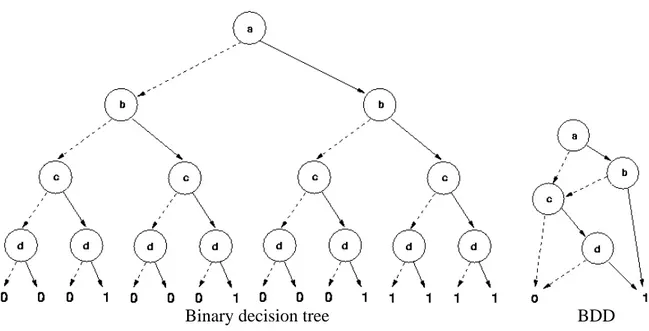
Binary decision diagrams (BDDs) are a canonical representation for boolean formulas [7]. A BDD is obtained from a binary decision tree by merging identical subtrees and eliminating nodes with identical left and right siblings. The resulting structure is a directed acyclic graph rather than a tree which allows nodes and substructures to be shared.
If the path end in the “leaf” labeled 0 then the formula will not be satisfied, conversely, if it end in the “leaf” labeled 1 then the formula will be satisfied - the assignment made to each variable satisfies the formula. Figure 2.2 illustrates the BDD for the boolean formula(a∧b)∨ (c∧d).
Figure 2.2: BDD for(a∧b)∨(c∧d)
Formally, a BDD is a directed acyclic graph with two kinds of vertex: non-terminal and ter-minal. Each non-terminal vertexv is labeled byvar(v), a distinct variable of the corresponding boolean formula. Each v has at least one incident arc (except the root vertex). Each v also has two outgoing arcs directed toward two children: lef t(v), corresponding to the case where var(v) = 0, andright(v), corresponding to the case wherevar(v) = 1.
A BDD has two terminal vertices labeled by 0 and 1, representing the truth value of the formula, respectively, false and true. For every truth assignment to the boolean variables of the formula, there is a corresponding path in the BDD from root to a terminal vertex. Figure 2.3 illustrates a BDD for the boolean formula(a∧b)∨(c∧d)compared to a Binary Decision Tree for this same formula.
BDDs are the main data structure of Symbolic Model Checking. They are an efficient way to represent boolean formulas. Often, they provide a much more concise representation than traditional representations, such as conjunctive normal forms and disjunctive normal forms.
BDDs are a canonical representation for boolean formulas. This means that two boolean formulas are logically equivalent if and only if its BDDs are isomorphic. This property simplifies the execution of frequent operations, like checking the equivalence of two formulas or deciding if a formula is satisfiable or not.
Binary decision tree BDD
Figure 2.3: Binary decision tree and a correspondent BDD for the formula(a∧b)∨(c∧d).
2.2.3
Specifying Properties of Concurrent Systems
In order to write specifications that describe properties of concurrent systems we need to define a set of atomic propositions AP. An atomic proposition is an expression that has the form
v op d wherev ∈V - the set of all variables in the system,d∈D- the domain of interpretation, and op is any relational operator. Now, we can formally define a Kripke structure M over AP as a four tupleM = (S, S0, R, L)where:
1. Sis a finite set of states.
2. S0 ⊆Sis the set of initial states.
3. R⊆S×Sis a transition relation that must be total.
4. L : 2AP is a function that labels each state with the set of atomic propositions true in that
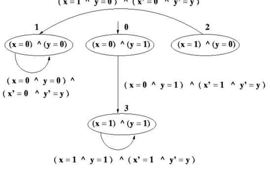
state.
To illustrate the notions defined we consider the simple system, where V = {x, y}, D = {0,1}andS0(x, y) ≡ (x = 0)∧(y = 1). The only possible transition isx =yrepresented by the formulaR(x, y, x′
, y′
)≡(x′
=y)∧(y′
=y).
The kripke structureM = (S, S0, R, L)extracted from these formula is:
• S ={(0,0),(0,1),(1,0),(1,1)}.
• S0 ={(0,1)}.
• L((0,0)) = {x = 0, y = 0}, L((0,1)) = {x = 0, y = 1},L((1,0)) = {x = 1, y = 0}, andL((1,1)) ={x= 1, y = 1}.
procedure exemplo; var
x := 0; y := 1; begin
while (true) x = y; end
The Figure 2.4 graphically shows the kripke structure M. As one can note the only path which starts in the initial state is (0,1)(1,1)(1,1)...(1,1). This is the only computation of the system.
Figure 2.4: The state transition graph
2.2.4
Temporal Logic
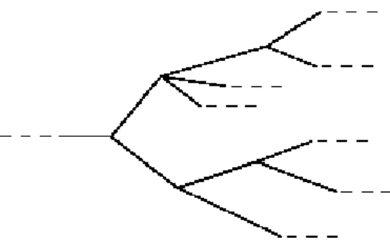
There exists several propositions of temporal logic [2]. These logics vary according temporal structure (linear or branching-time) and time characteristic (continuous or discrete). Temporal linear logics reason about the time as a chain of time instances. Branching-time logics reason about the time as having many possible futures at a given instance of time as shown in the Figure 2.5. Time is continuous if between two instances of time there is always another instance. Time is discrete if between two instances of time a third one can not be determined. In our work we used a branching-time and discrete logic known as Computation Tree Logic (CTL).
Figure 2.5: Linear and branching-time structure of time of temporal logics.
The Computation Tree Logic - CTL
Computation tree logic, is the logic used to express properties that will be verified by the model checker. Computation trees are derived from state transition graphs. The graph structure is unwound into an infinite tree rooted at the initial state, as seen in figure 2.6. Paths in this tree represent all possible computations of the program being modeled.
CTL provides operators to be applied over the paths formed by the computation tree. When these operators are specified in a formula they must appear in pair and in this order: path
quan-tifier followed by temporal operator. A path quanquan-tifier defines the scope of the paths over which
a formula f must hold. There are two path quantifiers: A, meaning all paths; and E, meaning some path. A temporal operator defines the appropriate temporal behavior that is supposed to happen along a path relating a formulaf. The temporal operators are the following:
• F (”in the future”or ”eventually”) - starting from the root,fholds in some state of the path;
Figure 2.6: State transition graph and corresponding computation tree.
• U (”until”) - there is a statesin the path where a formulag is satisfied and all predecessor states ofssatisfiesf.
• X (”next time”) - starting from the root,f holds in the second state of the path.
A well formed CTL formula is defined as follows:
1. Ifp∈AP, thenpis a CTL formula, such thatAP is the set of atomic propositions;
2. If f and g are CTL formulas, then ¬f, f ∨g, f ∧g, AFf, EFf, AGf, EGf, A[fRg], E[fRg], A[fUg], E[fUg], AXf, EXf, are CTL formulas.
Considering the Kripke modelM = (S, ρ, L)1, we denote thatM satisfies a CTL formulaf from a states∈S as
M, s|=f
Letf andgbe CTL formulas, the satisfaction relation|=is defined inductively as follows:
M, s|=p ⇔p∈L(s) M, s|=¬f ⇔M, s6|=f
M, s|=f∨g ⇔M, s|=f orM, s|=g M, s|=f∧g ⇔M, s|=f andM, s|=g
M, s|=AF f ⇔for all paths froms, sk ∈S is reachable andsk |=f M, s|=EF f ⇔for some path froms, sk∈S is reachable andsk |=f
M, s|=AGf ⇔for all pathsπ =s0s1s2. . . , si |=f, for alli≥0, ands0 =s
1
M, s|=EGf ⇔for some pathπ =s0s1s2. . . , si |=f, for alli≥0, ands0 =s M, s|=AXf ⇔for allsxsuch thatρ(s, sk)is defined,sk |=f
M, s|=A[f U g] ⇔for all pathsπ =s0s1s2. . . sk. . . , si |=f,0≤i < kandsk |=g M, s|=E[f U g] ⇔for some pathπ =s0s1s2. . . sk. . . , si |=f,0≤i < kandsk |=g
Despite all combinations we can get with path quantifiers and temporal operators presented above, we can express any CTL formula using∨,¬, EX, EU, EG [18]:
• AFf =¬EG¬f
• AGf =¬EF¬f
• AXf =¬EX¬f
• A[f Ug ]≡ ¬E[¬gU (¬f ∧ ¬g)]∧¬EG¬g
• EFf = E[⊤Uf]
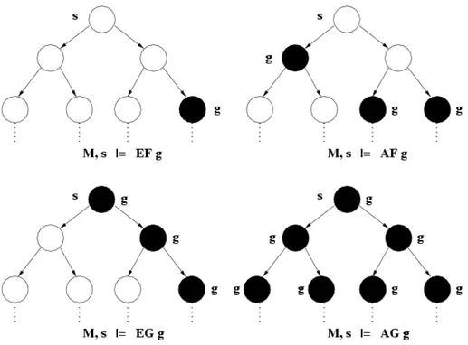
Figure 2.7 presents the computation of the most frequently used CTL operators. Some typical examples of CTL formulas relating to concurrent reactive systems are presented below:
• EF(started∧ ¬ready) - it is possible to get to a state wherestartedholds butready does not hold.
• AG(req →AF (ack)) - it is always the case that if the signalreq is high, then eventually ackwill also be high.
• A[greenLightUarmM oves] - it is always the case that the robot’s arm moves after the green light is on;
2.2.5
CTL Model Checking
CTL model checking consists of searching for Kripke model’s states with labelf, wheref is a CTL formula. The set of states labeled tofare the ones that satisfies the formula. Formally, let f be a CTL formula andlabel(s)be the set of sub formulas off that are true ins∈S. The CTL model checking problem is related to determining the setS ={s | M, s|=f → f ∈label(s)}. The model check process has two phases: translation and labeling. The translation phase consists of rewriting a CTL formula in terms of¬,∨, EX, EG, and EU. The labeling is a process ofi steps, where iis the number of sub formulas of f. In eachith step, thei−1 nested CTL operator (sub formula) labels a state if the sub formula is true in that state.
The labeling process observe the following rules:
Figure 2.7: Basic CTL operators over a computation tree. The ’s’ designates the state taken as root. The black states represent the states in which propositiongholds.
• labelsto¬f1, ifsis not labeled withf1
• labelstof1∨f2ifsis labeled withf1or withf2;
• labelsto EXf, iftis labeled withf andR(s, t);
• labelsto E[f1Uf2]
1. ifsis labeled withf2;
2. repeat backward from s: label t to E[f1 U f2] if t is labeled with f1 and exists a stateulabeled with E[f1Uf2], such thatR(t, u);
• labelsto EG[f]
1. label all states to EG[f];
2. delete EG[f] from any statesin which ifsis not labeled withf;
3. delete EG[f] from any statesif does not exist a statetlabeled with EG[f], such that R(s, t).
2.3
The SMV Language
In this section we briefly describe the SMV system [38] which we use to construct and verify formal models of e-commerce systems. A complete description can be found in Appendix A.
2.3.1
Introduction
The SMV system is a tool for checking finite state systems against specifications in the tem-poral logic CTL. The input language of SMV is designed to allow the description of finite state systems that range from completely synchronous to completely asynchronous, and from the de-tailed to the abstract. One can readily specify a system as a synchronous machine, or as an asynchronous network of abstract, nondeterministic processes. The language provides for mod-ular hierarchical descriptions, and for the definition of reusable components. Since it is intended to describe finite state machines, the only basic data types in the language are finite scalar types. Static, structured data types can also be constructed.
The logic CTL allows a rich class of temporal properties, including safety, liveness, fairness and deadlock freedom, to be specified in a concise syntax. SMV uses the OBDD-based symbolic model checking algorithm to efficiently determine whether specifications expressed in CTL are satisfied.
The primary purpose of the SMV input language is to provide a symbolic description of the transition relation of a finite Kripke structure. Any propositional formula can be used to describe this relation. This provides a great deal of flexibility, and at the same time a certain danger of inconsistency. For example, the presence of a logical contradiction can result in a deadlock - a state or states with no successor. This can make some specifications vacuously true, and makes the description unimplementable.
While the model checking process can be used to check for deadlocks, it is best to avoid the problem when possible by using a restricted description style. The SMV system supports this by providing a parallel-assignment syntax. The semantics of assignment in SMV is similar to that of single assignment data flow languages.
A program can be viewed as a system of simultaneous equations, whose solutions determine the next state. By checking programs for multiple assignments to the same variable, circular dependencies, and type errors, the compiler insures that a program using only the assignment mechanism is implementable. Consequently, this fragment of the language can be viewed as a hardware description language, or a programming language.
2.3.2
Input File
Consider the following example:
MODULE main
VAR
request : boolean;
state : { ready, busy };
ASSIGN
init(state) := ready;
next(state) := case
state = ready & request : busy;
1 : { ready, busy };
esac;
SPEC AG(request -> AF state = busy)
The input file describes both the model and the specification. The model is a Kripke structure, whose state is defined by a collection of state variables, which may be of Boolean or scalar type. The variable request is declared to be a Boolean in the above program, while the variable state is a scalar, which can take on the symbolic values ready or busy. The value of a scalar variable is encoded by the compiler using a collection of Boolean variables, so that the transition relation may be represented by an BDD. This encoding is invisible to the user, however.
The transition relation of the Kripke structure, and its initial state (or states), are determined by a collection of parallel assignments (a system of simultaneous equations), which are intro-duced by the keyword ASSIGN.
The Case Expression
case
state = ready & request : busy;
1 : { ready, busy };
esac;
The value of a case expression is determined by the first expression on the right hand side of a (:) such that the condition on the left hand side is true. Thus, if state = ready & request is true, then the result of the expression is busy, otherwise, it is the set{ready, busy}. When a set is assigned to a variable, the result is a non-deterministic choice among the values in the set. Thus, if the value of status is not ready, or request is false (in the current state), the value of state in the next state can be either ready or busy. Non-deterministic choices are useful for describing systems which are not yet fully implemented (i.e., where some design choices are left to the implementor), or abstract models of complex protocols, where the value of some state variables cannot be completely determined.
Notice that the variable request is not assigned in this program. This leaves the SMV system free to choose any value for this variable, giving it the characteristics of an unconstrained input to the system.
The SPEC Statement
The specification of the system appears as a formula in CTL under the keyword SPEC:
SPEC AG(request -> AF state = busy)
The SMV model checker verifies that all possible initial states satisfy the specification. In this case, the specification is that invariantly if request is true, then inevitably the value of state is busy.
2.3.3
Reusable Modules and Expressions
The following program illustrates the definition of reusable modules and expressions. It is a model of a 3 bit binary counter circuit. Notice that the module name main has special meaning in SMV, in the same way that it does in the C programming language. The order of module definitions in the input file is inconsequential.
MODULE main
VAR
bit0 : counter.cell(1);
bit2 : counter.cell(bit1.carry.out);
SPEC
AG AF bit2.carry.out
MODULE counter.cell(carry.in)
VAR
value : boolean;
ASSIGN
init(value) := 0;
next(value) := value + carry.in mod 2;
DEFINE
carry.out := value & carry.in;
In this example, we see that a variable can also be an instance of a user defined module. The module in this case is counter cell, which is instantiated three times, with the names bit0, bit1 and bit2.
The counter cell module has one formal parameter carry in. In the instance bit0, this formal parameter is given the actual value 1. In the instance bit1, carryin is given the value of the expression bit0.carry out. This expression is evaluated in the context of the main module.
However, an expression of the form a.b denotes component b of module a, just as if the module a were a data structure in a standard programming language. Hence, the carry in of module bit1 is the carry out of module bit0.
The keyword DEFINE is used to assign the expression value & carry in to the symbol carry out. They are analogous to macro definitions, but notice that a symbol can be referenced before it is defined. The effect of the DEFINE statement could have been obtained by declaring a variable and assigning its value, as follows:
VAR
carry.out : boolean;
ASSIGN
carry.out := value & carry.in;
Notice that in this case, the current value of the variable is assigned, rather than the next value. Defined symbols are sometimes preferable to variables since they do not require introducing a new variable into the OBDD representation of the system.
typed, definitions are not. This may be an advantage or a disadvantage, depending on your point of view.
In a parallel-assignment language, the question arises: What happens if a given variable is
assigned twice in parallel? More seriously: What happens in the case of an absurdity, like a := a + 1; (as opposed to the sensible next(a) := a + 1;)?
In the case of SMV, the compiler detects both multiple assignments and circular dependen-cies, and treats these as semantic errors, even in the case where the corresponding system of equations has a unique solution. Another way of putting this is that there must be a total order in which the assignments can be executed which respects all of the data dependencies. The same logic applies to defined symbols. As a result, all legal SMV programs are realizable.
2.3.4
Asynchronous Execution
By default, all of the assignment statements in an SMV program are executed in parallel and simultaneously. It is possible, however, to define a collection of parallel processes, whose actions are interleaved arbitrarily in the execution sequence of the program. This is useful for describing communication protocols, asynchronous circuits, or other systems whose actions are not synchronized (including synchronous circuits with more than one clock). This technique is illustrated by the following program, which represents a ring of three inverting gates.
MODULE main
VAR
gate1 : process inverter(gate3.output);
gate2 : process inverter(gate1.output);
gate3 : process inverter(gate2.output);
SPEC
(AG AF gate1.out) & (AG AF !gate1.out)
MODULE inverter(input)
VAR
output : boolean;
ASSIGN
init(output) := 0;
next(output) := !input;
assignment statements in that process in parallel. It is implicit that if a given variable is not assigned by the process, then its value remains unchanged. Because the choice of the next process to execute is non-deterministic, this program models the ring of inverters independently of the speed of the gates. The specification of this program states that the output of gate1 oscillates (i.e., that its value is infinitely often zero, and infinitely often 1). In fact, this specification is false, since the system is not forced to execute every process infinitely often, hence the output of a given gate may remain constant, regardless of changes of its input.
In order to force a given process to execute infinitely often, we can use a fairness constraint. A fairness constraint restricts the attention of the model checker to those execution paths along which a given CTL formula is true infinitely often. Each process has a special variable called running which is true if and only if that process is currently executing. By adding the declaration:
FAIRNESS running
to the module inverter, we can effectively force every instance of inverter to execute infinitely often, thus making the specification true.
One advantage of using interleaving processes to describe a system is that it allows a partic-ularly efficient OBDD representation of the transition relation. We observe that the set of states reachable by one step of the program is the union of the sets of states reachable by each individual process. Hence, rather than constructing the transition relation of the entire system, we can use the transition relations of the individual processes separately and the combine the results [34]. This can yield a substantial savings in space in representing the transition relation.
The alternative to using processes to model an asynchronous circuit would be to have all gates execute simultaneously, but allow each gate the non-deterministic choice of evaluating its output, or keeping the same output value. Such a model of the inverter ring would look like the following:
MODULE main
VAR
gate1 : inverter(gate3.output);
gate2 : inverter(gate2.output);
gate3 : inverter(gate1.output);
SPEC
(AG AF gate1.out) & (AG AF !gate1.out)
MODULE inverter(input)
VAR
ASSIGN
init(output) := 0;
next(output) := !input union output;
The union operator allows us to express a nondeterministic choice between two expressions. Thus, the next output of each gate can be either its current output, or the negation of its current input - each gate can choose non-deterministically whether to delay or not. As a result, the num-ber of possible transitions from a given state can be as high as 2n, where n is the numnum-ber of gates. This sometimes (but not always) makes it more expensive to represent the transition relation. The relative advantages of interleaving and simultaneous models of asynchronous systems are discussed in [33].
2.3.5
Counterexample
If any specification in the program is false, the SMV model checker attempts to produce a counterexample, proving that the specification is false. This is not always possible, since formulas preceded by existential path quantifiers cannot be proved false by a showing a single execution path. Similarly, sub-formulas preceded by universal path quantifier cannot be proved true by a showing a single execution path. In addition, some formulas require infinite execution paths as counterexamples. In this case, the model checker outputs a looping path up to and including the first repetition of a state.
Although the parallel assignment mechanism should be suitable to most purposes, it is pos-sible in SMV to specify the transition relation directly as a propositional formula in terms of the current and next values of the state variables. Any current/next state pair is in the transition relation if and only if the value of the formula is one.
2.3.6
Summary
The SMV language is designed to be flexible in terms of the styles of models it can describe. It is possible to fairly concisely describe synchronous or asynchronous systems, to describe detailed deterministic models or abstract nondeterministic models, and to exploit the modular structure of a system to make the description more concise. It is also possible to write logical ab-surdities if one desires to, and also sometimes if one does not desire to, using INIT declarations. By using only the parallel assignment mechanism, however, this problem can be avoided.
Figure 2.8: Kripke structure representing a microwave.
Since the full generality of the symbolic model checking technique is available through the SMV language, it is possible that translators from various languages, process models, and inter-mediate formats be created. In particular, existing silicon compilers could be used to translate high level languages with rich feature sets into a low level form that could be readily translated into the SMV language.
2.4
A Microwave Example
This Section presents an example of verification using CTL logic. The example is about a simplified microwave inspired in a similar one given by Clarke, Grumberg, and Peled [18].
The microwave is described by three boolean variables. The variable setup-ed represents the parameters of the microwave, such as time of cooking, set by user. Door-opened is the variable that indicates whether the microwave’s door is opened or not. The variable cooking states if the microwave is cooking the meal.
have false value.
The Kripke structure of Figure 2.8 models the main operation of a microwave. We can open or close the microwave’s door. We can set the time of cooking. We can cook. We can pause or cancel the cooking and restarting the cooking again. The microwave turn itself off after the cooking time (timeout).
A very important (life) safety property of any microwave is being free of cooking with its door opened. We can verify this property with CTL logic by expressing
AG(cooking→ ¬doorOpened)
We can simplify this formula in terms of equivalent ones:
AG(cooking → ¬doorOopened)≡ ¬EF¬(cooking→ ¬doorOpened)≡ ¬EF¬(¬cooking∨ ¬doorOpened)≡ ¬EF(cooking∧doorOpened)
Chapter 3
Web Based Systems’ Modeling
There are many types of transactional systems. Web based applications, such as digital li-brary, virtual bookstore, and auction sites are examples. Most web applications can be modeled using a few entities: the products being commercialized such as books or DVDs, the actors that act upon these products such as consumer or seller, and the actions that modify the state of the product such as reserving or selling an item [45, 46].
For example, similarly to traditional commercial systems the main entity of electronic com-merce system is the product that is transactioned. For each product being commercialized there are one or more items, which are instances of the product. Each item is characterized by its life cycle, which can be represented by a state-transition graph, i.e., the states assumed by the item while being commercialized and the valid transitions between states. Examples of states are reserved or sold. The item’s domain is the set of all states the item can be in.
The entities that interact with the system are called actors. Examples of actors are buyers, sellers and the store’s manager. The actors perform actions that may change the state of an item, that is, actions correspond to transitions in the life cycle graph. Putting an item in the basket or canceling an item’s reserve are examples of actions.
Services are sequences of actions on products. While each action is associated with an item and usually comprises simple operations such as allocating an item for future purchase, services handle each product as a whole, performing full transactions. Purchasing a book is an example of a service, which consists of paying for the book, dispatching it, and updating the inventory.
The main difference between web systems are their nature and their business rules - a busi-ness rule is a norm that specifies some functioning of an application. Some busibusi-ness rules are common, for example: an item should not be sold to more than one customer. On the other hand, there are many other rules specific to the application, as to allow or not the reservation of an item, to provide supply control, or to define priority to transactions executed concurrently.
example, rules can be described as formulas in CTL, which are built from atomic propositions, boolean connectives, and temporal operators as described in the last Chapter.
Consider the following example: an item can only be reserved if it is available. To specify this property, a developer would have to translate this informal requirement into the following CTL formula:
AG (((state = available) & (action = reserve) & (inventory>0))→AX ((state = reserved) & (next(inventory) = inventory - 1))).
As one can see, the specification process demands expertise in formal methods. Acquiring this level of expertise represents an obstacle to the adoption of any methodology. As it is usually difficult to read and understand formulas written in temporal logic, and even more difficult to write them correctly without the knowledge in the syntax of the specification language, we have proposed in [52] a pattern system to overcome such problems.
3.1
Properties
It is well known that any transactional system [3] must satisfies certain characteristics tradi-tionally grouped into four properties under the acronym ACID (atomicity, consistence, isolation and durability). In our work we are particular interested in verifying three important types of properties related to transactions:
• Atomicity: A transaction must be finished or not started, that is, if it does not finish, its effects have to be undone.
• Consistency: A transaction transforms a consistent state into another consistent one, with-out necessarily preserving the consistency in the intermediate points of the transaction. The state must remain coherent at the end of an execution.
• Isolation: The result of one transaction must not affect the result of another concurrent transaction - its effect is not visible to other transactions until the transaction is completed.
These properties are related to the correctness of the model and assert that all states and actions are achieved. Transitivity, for example, is a consistency property which defines the next state to be achieved after the occurrence of an event in the current state. It is necessary to check its veracity to guarantee the correct execution of actions.
Web based applications are examples of transactional systems. In this case, a transaction can be seen as a sequence of actions affecting the existing items, each action potentially modifying its state. One of the most important properties that must be satisfied in this context is the guarantee that the transactions being executed are consistent. One must show that the concurrency control mechanism implemented is correct and that concurrent transactions do not interfere with each other.
3.2
The Formal-CAFE Methodology
The Formal-CAFE methodology [46] is an extension of the CAFE methodology [32]. The main idea of Formal-CAFE is to design e-commerce systems applying model checking. The
CAFE methodology explains how to specify an e-commerce system and it considers that the user
knows some formal language, such as SMV [33], to build the model. Table 3.1 presents the elements used to compose an e-commerce system specification according to Formal-CAFE.
Level Components Conceptual Entities Application Product’s item
life cycle of negotiated item Actions
Actors Functional Services
Products Product’s items
Functional requirements Execution System’s architecture
Components Protocols
Table 3.1: Elements of Formal-CAFE’s methodology
3.2.1
Conceptual Level
Formally, Formal-CAFE characterizes an e-commerce system by a tuple < P, I, D, Ag, Ac, S >, whereP is the set of products,I is the set of items,D is the set of product domains, Agis the set of actors,Acis the set of actions andSis the set of services.
Products are sets of items, that is, i∈ I means thati ∈p, p ∈P. The products partition the set of items, that is, every item belongs specifically to a single product. Formally,I = S∀p∈P p
andpi∩pj =∅fori6=j. Domains are associated with items, that is, each itemiis characterized
by a domainDi. Two items of the same product have the same domain, i.e., for all itemsi, j ∈I,
there is a productpsuch that ifi∈pandj ∈p, thenDi =Dj.
3.2.2
Application Level
This level describes the e-commerce system in terms of the life cycle of the items. It is necessary to identify the states of an item, its attributes, and the set of actions that could be executed on it such as:
Innocuous actions: they do not affect the state of an item.
Temporary actions: they change the state of the item temporarily - the item can assume its original state again.
Perennial actions: they change the state of the item in permanent character, being irreversible.
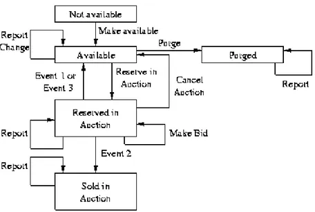
The items are modeled by their life cycle graphs, which represent the state each item can be in during its life cycle in the system. An example of a life cycle graph can be seen in Figure 3.1. States in this graph are possible states for the item such as available, or reserved. Transitions represent the effect of actions such as reserving an item or buying it.
Each action is associated with a transition in the state-transition graph of the item and is defined by a tuple < a, i, tr >∈ Ac, where a ∈ Ag is the actor that performs the action, and i∈Iis the item over which the action is performed, andtr∈DixDi is the transition associated
with the action. In our model, the actions performed on a given item are totally ordered, that is, for each pair of actionsxandy, whereix andiy are the same, eitherxhas happened beforeyor yhas happened beforex.
Services are defined by tuples < p, A >, where p ∈ P and A = a1, a2, . . . is a sequence
of actions such that ifai = (d1, d2), ai+1 = (d3, d4)thend2 = d3 ∀i, di ∈ Dj whereDj is the
domain of an item fromp.
Figure 3.1: The life cycle graph of product’s item
In this model, each global state represents one state in each product life cycle graph, and tran-sitions model the effects of actions in the system. Therefore, paths in the global graph represent events that can occur in the system. The life cycle of the product is the set of all life cycles of its items.
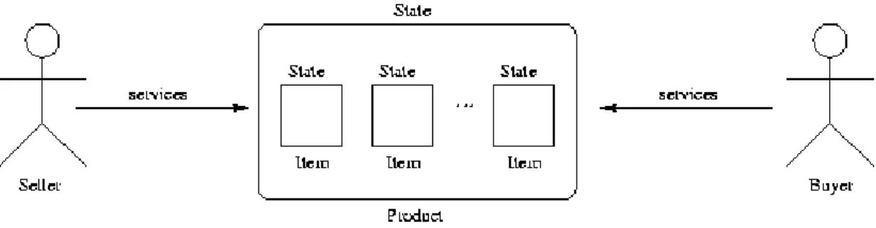
The Figure 3.2 illustrates the second level of the methodology. As this figure shows, there are actors (Seller and Buyer) that represent the consumer and the supplier of the system. There is an item, which has a set of states. The actors execute actions that could affect the item’s state.
Figure 3.2: The Second Level of the Methodology
3.2.3
Functional Level
This level introduces the product, composed by zero (the product is not available) or more items. The designer determines the operations the actors can perform (services). A service is executed on products and its effects might change or not the state of it and its items.
The actors execute services that change the state of the item. This state must be consistent
with the life cycle of the item and the related business rule associated. So, the transitivity property