✡✡✡ ✪✪
✪ ✱✱
✱✱ ✑✑✑ ✟✟ ❡
❡ ❡ ❅
❅❅ ❧
❧ ❧ ◗
◗◗ ❍ ❍P P P ❳❳ ❳ ❤❤ ❤ ❤
✭ ✭ ✭
✭✏✟✏
IFT
Universidade Estadual PaulistaInstituto de F´ısica Te´oricaDISSERTAC¸ ˜AO DE MESTRADO IFT–D.005/13
Anti-de Sitter Holography in Different Coordinates
Ricardo Alfonso Hern´andez Moreno
Orientador
Horat¸iu Stefan Nˇastase
Acknowledgments
I would like to thank all the people who somehow contributed to the development of this dissertation. All my gratitude to Prof. Dr. Horatiu Nastase for the advisement during these 2 years and his unconditional support; to the Professors I met at the IFT; to the staff and of course to my closer colleagues: Cuper, David, Fernando, John, Prieslei, Rodolfo, etc. In general, I thank the kind community at the IFT.
All my work is dedicated to my family, friends and Estefan´ıa.
”We fought far under the living earth, where time is not counted.”
Resumo
O objetivo deste trabalho ´e mostrar a importˆancia da escolha do sistema de co-ordenadas e assinatura para descrever o espa¸co Anti-de Sitter na Correspondˆencia AdS/CFT. Para fazer isto, mostraremos como calcular correlatores em diferentes co-ordenadas no lado gravitacional da correspondˆencia. Em particular, apresentamos o procedimiento geral para encontrar o propagador bulk-fronteira para um campo es-calar, de gauge e espinorial usando o m´etodo de Witten em coordenadas de Poincar´e com assinatura euclideana. Tamb´em mostramos os c´alculos das fun¸co˜es de npontos para um campo escalar interagente em AdS a n´ıvel de ´arvore e comparamos os resul-tados com os v´ınculos da teor´ıa de campos conformes. Para comparar as implica¸co˜es de trabalhar em outro sistema coordenado refazemos os c´alculos dos propagadores para o campo escalar em coordenadas globais. Finalmente mostramos como cal-cular o propagador bulk-fronteira para um campo 3-forma que vive em AdS7 em
coordenadas globais e de Poincar´e.
Palavras Chaves: Espa¸co Anti-de Sitter; Teor´ıa de Campos Conformes; Corre-spondˆencia AdS/CFT
´
Abstract
The goal of this work is to show the significance of the choice of coordinates system and signature to describe the Anti-de Sitter space within AdS/CFT Correspondence. In order to do so, we will show how to calculate AdS/CFT correlators in different coordinates from the gravity side of the correspondence. In particular, we present the general procedure to find the bulk-to-boundary propagators for scalar, gauge and spinor fields using Witten’s method in Poincar´e coordinates with Euclidean sig-nature. We also show the calculations ofn-point functions for a classical interacting scalar field in AdS at tree level and compare the results with the CFT constraints. To compare the implications of working in different coordinates, we recalculate the propagators for the scalar field in Global coordinates. Finally, we show the cal-culations of bulk-to-boundary propagator for a 3-form field living in AdS7 in both
Contents
1 Introduction 1
2 Anti-de Sitter Spaces 3
2.1 AdS as exact solution of Einstein Equations . . . 4
2.2 AdS as embedding . . . 4
2.3 Systems of coordinates and signatures . . . 5
2.4 Causal Structure . . . 5
2.5 Boundaries . . . 8
2.6 More properties of AdS spaces . . . 10
3 Conformal Field Theory 11 3.1 Conformal group . . . 11
3.2 Conformal Invariance . . . 13
4 The AdS/CFT Correspondence 16 4.1 Physics in AdS is holographic . . . 16
4.2 Example . . . 16
4.3 Witten’s prescription . . . 17
4.4 Extra . . . 19
5 Holography 21 5.1 Holography for Scalar Fields . . . 21
5.2 n-point functions for Scalar Fields . . . 24
5.3 Holography for Gauge Fields . . . 33
5.4 Holography for Spinor Fields . . . 38
6 Holography in different Coordinates 43 6.1 Scalar fields in Lorentzian Poincar´e Coordinates . . . 44
6.2 Scalar fields in Global Coordinates . . . 45
7 Propagators for p-forms in AdS2p+1: An Example 51
8 Conclusions 61
A Bessel Functions 62
C Bitensors and limits 64
1
Introduction
AdS plays a role in the AdS/CFT which is simply far from trivial.
This dissertation is organized as follows: The first chapter has to do with Anti-de Sitter space (AdS), we start Anti-defining what AdS is within general relativity, how it can be derived as a solution of Einstein equations or by embedding of a hyper-surface in certain ambient space, later we present the different coordinates system of our interest to describe this space and analyze the causal structure by using Penrose diagrams, we end this section studying the boundary of AdS and what changes with every coordinates we consider. In the next chapter we present the basics of conformal field theory (CFT), starting from the definitions of conformal transformations of coordinates, its general group properties and how a field theory with conformal invariance is restricted, this is done by studying the constraints imposed on then-point functions working in the coordinate representation. Once we study AdS and CFT separately we are ready to say some words about the AdS/CFT Correspondence. Its discovery and foundations are beyond the scope of the intended work, so we only mention what it means, we present the most known and studied example and we develop the prescription proposed by Wit-ten in [2] which serves as a recipe to match observables of the two sides of the correspondence. Following, we find a chapter treating holography, basically we compute bulk-to-boundary propagators in Poincar´e coordinates for scalars, gauge and spinor fields living in AdS, as well as 2-point functions at tree level, which results are compared with functional form dictated by conformal invariance. A general formula to compute n-point for scalars at tree level is also found. Be-sides, in this chapter we check the relations between scaling dimension and the mass according to the AdS/CFT dictionary. In chapter 6 we deal with one of the main topics of this work, holography in other coordinates systems than Euclidean Poincar´e coordinates. We start by solving the equation of motion for a free scalar field living on AdS with Minkowski signature and we see that consistency requires the inclusion of new ”objects” which were not present in the Euclidean case. In this section we also solve the Klein-Gordon equation with global AdS background and we find the new bulk-to-boundary propagator which relation with the one found in the euclidean Poincar´e is, as expected, far from being a simple coordi-nate transformation. In the last chapter we present an example of correspondence different from the well-known case [1] and we calculate the bulk-to-boundary prop-agator for a 3-form living inAdS7 in Poincar´e coordinates and finally we compute
2
Anti-de Sitter Spaces
General relativity is the theory that describes the dynamics of space-time, it is based on the Einstein equations (1) which gives the space-time metricgab once the
content of matter Tab is known.
Rab−
1
2Rgab+ Λgab = 8πTab (1) Exact solutions of (1) are more likely found for spaces of high symmetry, in particular we are interested in spaces with constant curvature. To be an exact solution,Tab must be the energy momentum tensor of some configuration of matter
which does not violate local causality and it is also restricted to forms in which the energy density measured by any observer would not be negative.
Once a solution is found, we would like to describe physical objects living on the this space-time, so we consider the line element also called the metric:
ds2 =gabdxadxb (2)
We can describe a space as a surface living inside some background space, or embedding space. For instance, the curved 2d surface space of the 2-sphere can be regarded as living on the 3d euclidean space (3) supplemented with an extra condition (4).
ds2 =dx2+dy2+dz2 (3)
x2+y2+z2 =R2 (4) Then, the 2-dimensional metric is given by:
ds2 =dx2(1 + x2
R2−x2−y2) +dy
2(1 + y2
R2−x2−y2) + 2dxdy
xy
R2−x2−y2 (5)
Another example is the Lobachevski space, which has negative curvatureR <0 (two parallel geodesics diverge), this is a 2d space described by embedding the surface (6) into a 3d Minkowski space (7).
x2+y2−z2 =−R2 (6)
2.1
AdS as exact solution of Einstein Equations
Anti-de Sitter space is the simplest, maximally symmetric solution of the Einstein equation with negative curvature. Locally, spacetime metrics of constant curvature are characterized by :
Rabcd =
1
d(d−1)R(gacgbd−gadgbc) (8) which is equivalent to:
Rab−
1
2Rgab =− 1
4Rgab (9)
Comparing this with Einstein equation we can consistently identify these spaces as solutions with Λ = 14R for an empty space Tab = 0. For the case R < 0 we
obtain the so-called Anti-de Sitter space(AdS) .
2.2
AdS as embedding
AdS space is represented by a Lorentzian version of Lobachevski space given by the embedding ind+ 1 dimensions:
−X02+
d−1
X
i
Xi2−Xd+12 =−R2 (10)
ds2 =−dX2
0 +
d−1
X
i
dX2
i −dXd+12 (11)
Then, denoting Xµ = (X0, Xd+1, X1, . . . , Xd−1) we see that by construction it
2.3
Systems of coordinates and signatures
We can solve the embedding equations with the so called global coordinates:
X0 =Rcoshρcosτ
Xi =RsinhρΩi
Xd+1 =Rcoshρsinτ
(12)
where 0≤ρ <∞, 0≤τ < 2π and −1≤Ωi ≤1 with the additional condition
P
iΩi = 1. Then the metric can be written as:
ds2 =R2 −cosh2ρdτ2+dρ2+ sinh2ρdΩ2d−1
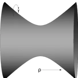
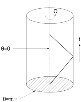
(13) With τ ∈[0,2π) we are covering the space once, that is why these coordinates are called Global. In these coordinates AdS can be represented by the hyperboloid shown in the Figure 1. We also see that the ambient space has two times, but the hyperboloid only one (they are orthogonal to each other). Nonetheless , there is a problem as we approach at ρ≈0 :
ds2 =R2 −dτ2+dρ2+ρ2dΩ2d−1
(14) Which means we obtain a space S1×Rd−1 and therefore we could have closed
time-like curves which are prohibited because of causal concerns. We can solve this by unwrapping the circle, it means letting −∞ < τ < ∞ and we obtain the “universal cover” of global AdS, where we do not have closed time-like curves. So in this work whenever we mention global AdS we refer to its universal covering space. We can also compute the curvature for this metric and check that this space has a constant negative curvature Λ = −d(d+1)R2 .
2.4
Causal Structure
Penrose diagrams are an important tool developed by Penrose with the aim to understand the causal structure of a spacetime. We are interested in studying AdS spaces and in order to do that it is easier to start with the simpler cases. First, we are going to study the Penrose diagram of flat Minkowski space R1,p
which metric in two dimensions is given by
Figure 1: AdS Space in Global coordinates
ds2 =−du+du− (16)
where again −∞ < u± < ∞. Now, it is easy to show that by making u± =
tan (τ ±θ)/2 we get:
ds2 = Ω2(τ, θ)(−dτ2+dθ2) (17) with
Ω2(τ, θ) = 1 4sec
2 1
2(τ +θ) sec
2 1
2(τ −θ) (18) where |τ ±θ|< π.
Since light ray trajectories (ds2 = 0) are not affected by conformal factors in the
metric, we can map Minkowski space into the full diamond region|τ±θ|< πin the Figure 2 and analyze the causal structure of the space. The two corners i0 where
(τ, θ) = (0,±π) represent the two spacelike infinities that correspond to x=±∞, and i± the future and past timelike infinity. This procedure is used to define
Figure 2: Penrose diagram of R1,1
Now let us analyze the case of Minkowski in arbitrary dimensions R1,p and
p≥2. In spherical coordinates the metric is given by
ds2 =−dt2+dr2+r2dΩ2p−1 (19) where 0 < r < ∞ and at every point (r, t) there is a sphere Sp−1, so we can
focus on the (r, t) portion. We obtain the same results as in previous case of R1,1
where|τ±θ|< π, but nowθ is restricted to θ >0 and the Penrose diagram is the triangle in the figure 3. Explicitly, the conformal scaled metric will be given by:
ds2 =−dτ2+dθ2+ sin2θΩ2p−1 (20) We can analytically continue this space outside the triangle by letting −∞< τ <∞and 0 ≤θ≤π and we obtain the geometry ofR×Sp which is the Einstein
static universe.
Now for the case of AdS in global coordinates first we would like to mapρ=∞ to a finite distance, then we set tanθ = sinhρ, with 0 ≤ θ ≤ π/2, except in the 2-dimensional case which is special and allows−π/2≤θ ≤π/2. For this we have:
ds2 = R
2
cos2θ −dτ
2+dθ2+ sin2θdΩ2 d−2
(21) Dropping the conformal factor we obtain:
Figure 3: Penrose diagram of R1,d
We notice that this is the same metric of the Einstein static universe found above with a one less dimension. Nevertheless, in this case of AdS the θ coordi-nate takes different values, more exactly conformal AdSd+2 can be mapped to a
half of the Einstein static universe. This can be used to define spaces which are asymptotically AdS: It is a spacetime which is conformal to a region with the same boundary structure of one half of the Einstein static universe.
2.5
Boundaries
Let us look at AdS3 which will have a boundary at θ =π/2 and we obtain ds2 =
−dτ2+dΩ2. So the boundary has the topologyR×S, in general the boundary of
AdSd+1 in global coordinates is R×Sd−1
We would not like to deal with a theory defined on spheres, then we choose coordinates in which the boundary metric is flat space, it can be Minskowski or Euclidean space. The coordinates system chosen is called Poincar´e coordinates.
The Poincar´e coordinates are defined by:
X0 =
z
2
1 + 1
z2 R
2+~x2−t2
Xd−1 =
z
2
1− 1 z2 R
2−~x2+t2
Xd+1=
Rt z
Xi =
Rxi
z
We notice that :
1
z =
X0−Xd−1
R2 (24)
So we can choose the sign ofz and that will describe only half the hyperboloid, this equation also tell us that the region z = 0 does not belong to AdS space. Usually people work withz >0.
Figure 4: Diagram of the global AdS boundary and the Poincar´e patch
We obtain:
ds2 = R
2
z2(−dt
2+
d−1
X
i
dx2i +dz2)
=R2 z2(−dt2+ d−1
X
i
dx2 i) +
dz2
z2
! (25)
Now the boundary is located at z = 0 and it has the topology R1,d. One of
the points we would like to stress in this section is that Anti-de Sitter space in Poincar´e coordinates is a patch which is a subset of the whole global AdS.
Figure 5: Penrose diagram for Poincar´e AdS
in particular we are interested in the case where p = 3, and then SO(2,4) is the isometry group ofN = 4 SY M in 4d.
2.6
More properties of AdS spaces
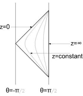
The Penrose diagram of AdS2 (Figure 5) is an infinite strip between θ = −π/2
and θ =π/2 (τ is arbitrary) in global coordinates. If we do the same in Poincar´e coordinates we realize that in these coordinates the Penrose diagram is only portion (triangle) of the strip.
3
Conformal Field Theory
In this chapter we develop the basics of one of the two sides of the AdS/CFT Correspondence, we will sutdy the definition of conformal transformations, its properties within group theory and the constraints of conformal invariance on field theories. It is relevant to mention that along this work we are going to check the conformally invariant structure of the correlation functions calculated in classical supergravity on AdS background, therefore the natural choice is to work in the coordinate representation.
3.1
Conformal group
Let us start by studying the conformal group and its representations. A general coordinate transformation xµ→x′
µ is such that metric transforms as
g′µν(x′) = ∂x
α
∂x′µ
∂xβ
∂x′νgαβ(x) (26)
The conformal group of transformations is a subgroup of the global coordinate transformations such that they leave the metric invariant up to a scale change Ω that can depend on the coordinates:
gµν′ (x′) = Ω(x)gµν(x) (27)
Considering an infinitesimal transformation x′µ = xµ+ǫµ(x), which together
with (26) leads to:
∂µǫν+∂νǫµ =
2
d(∂·ǫ)ηµν (28)
For d ≥ 3 we find (d−1)(∂ ·ǫ) = 0 and we can make the ansatz ǫµ(x) =
aµ+bµνxν +Cµνρxνxρ.
As special cases we have:
T ranslations ǫµ(x) = aµ
Rotations ǫµ(x) = ωνµxν
Dilations ǫµ(x) = λxµ
Special Conf ormal T ransf ormations ǫµ(x) = bµx2−xµb·x
(29)
Pµ =−i∂µ
Mµν =i(xµ∂ν −xν∂µ)
D =ixµ∂ µ
Kµ =−i(x2∂µ−2xµxν∂ν)
(30)
And the non vanishing commutation rules define the algebra:
[D, Pµ] =iPµ
[D, Kµ] =−iKµ
[Kµ, Pν] = 2i(ηµνD−Mµν)
[Kρ, Mµν] =i(ηρµKν −ηρνKµ)
[Pρ, Mµν] =i(ηρµPν −ηρνPµ)
[Mµν, Mρσ] =i(ηνρMµσ−ηνσMµρ+ηµσMνρ−ηµρMνσ)
(31)
These conform the algebra of the conformal group, we are specially interested in [D, Mµν] = 0 which means D is an scalar and also [D, Pµ] =iPµ, [D, Kµ] =−iKµ
which will help us to construct representations of the conformal group.
We must diagonalize the dilation operator and label states with the eigenvalue ∆, remember these operator represents a scale transformation so we call ∆ scaling dimension.
The commutation relations show that Pµ raises the dimension of the field and
Kµ lowers it. Unitary representations are constructed with the assumption that
there is a state with the lowest scaling dimension ∆, such state is called conformal primary.
[Pµ,Ψ(x)] =i∂µΨ(x)
[Mµν,Ψ(x)] = [i(xµ∂ν−xν∂µ) + Σµν]Ψ(x)
[D,Ψ(x)] =i(−∆ +xµ∂µ)Ψ(x)
[Kµ,Ψ(x)] = [i(x2∂µ−2xµxν∂ν + 2xµ∆)−2xνΣµν]Ψ(x)
(32)
From previous analysis of commutation relations we notice that given Ψ(x) with conformal dimension ∆, this state is not an eigenfunction of the Hamiltonian
H =P0neither has a massM associated. Then if we want to label states belonging
to some representation of the conformal group, we might use the scaling dimension ∆, the Lorentz numbers associated withMµν and the additional internal quantum
3.2
Conformal Invariance
A field theory with conformal invariance must fulfill several requirements, among them: φj a set of fields called “quasi-primary” that under global conformal
trans-formations, considering spinless field for simplicity:
φj(x)→
∂x′ ∂x
∆j/d
φj(x′) (33)
where ∆j represents the conformal(scaling) dimension of the field φj. Then
correlation functions must transform as:
hφ1(x1)φ2(x2). . . φn(xn)i=
∂x′ ∂x
∆1/d
x=x1 ∂x′ ∂x
∆2/d
x=x2 . . . ∂x′ ∂x
∆n/d
x=xn
hφ1(x′1)φ2(x′2). . . φn(x′n)i
(34) Because of the group invariance we find that two quasi-primary fields are cor-related if they have the same scaling dimension ∆.
As a result of conformal invariance, the functional forms of n-point functions of quasi-primary fields are severely restricted. For simplicity, let us first analyze the case of spinless objects, namely conformal invariant correlators for scalar fields: Translation invariance dictates thatn-point functions only depend on the distances
xi−xj, rotational invariance tell us that they can only depend on rij =|xi−xj|,
scale invariance says that correlation can only depend on the ratios rij/rlm and
special conformal transformations impose the dependence on the so called cross-ratios rijrlm/rilrjm. [14]
For the case of the 2-point function we get hφ1(x1)φ2(x2)i= C12ra12, with C12
a constant and a a power to be determined, and conformal invariance requires:
hφ1(x1)φ2(x2)i=
∂x′ ∂x
∆1/d
∂x′ ∂x
∆2/d
hφ1(x′1)φ2(x′2)i (35)
If the conformal transformation is a scale transformation Ω =λ−2 then ∂x
′
∂x
=
Ω−d/2 =λd we obtain:
hφ1(x1)φ2(x2)i=λ∆1+∆2C12 r
′a
12 =λ∆1+∆2λaC12 r12a (36)
So we must have −a = ∆1+ ∆2 and so:
hφ1(x1)φ2(x2)i=
C12
r∆1+∆2
12
We can restrict even more our correlator by using invariance under special conformal transformations. We have that:
(r′12)2 = (r12)
2
(1 + 2b·x1+b2x21)(1 + 2b·x2+b2x22)
(38) and also:
C12
r∆1+∆2
12
= 1
(1 + 2b·x1+b2x21)∆1
1
(1 + 2b·x2 +b2x22)∆2
C12
r′∆1+∆2
12
(39)
Combining the two we get:
1 = (1 + 2b·x1+b2x21)
∆1+∆2−2∆1
2 (1 + 2b·x
2+b2x22)
∆1+∆2−2∆2
2 (40)
Therefore, if C12 6= 0 then ∆1 = ∆2 = ∆ and so we obtain:
hφ1(x1)φ2(x2)i=
C12
(r12)2∆
(41)
and the constant can be determined by the normalization condition of the fields.
The 3-point function is similarly restricted by conformal invariance, in general we have
hφ1(x1)φ2(x2)φ3(x3)i=
X
a,b,c
Cabc
(r12)a(r23)b(r13)c
(42)
In this case scale transformations invariance says a+b+c = ∆1 + ∆2+ ∆3.
Special conformal transformations gives a= ∆1+ ∆2−∆3,b = ∆2+ ∆3−∆1 and
c= ∆1+ ∆3+ ∆2. So the general form is:
hφ1(x1)φ2(x2)φ3(x3)i=
C123
(r12)∆1+∆2−∆3(r23)∆2+∆3−∆1(r13)∆1+∆3+∆2
(43)
The functional forms are more complicated por n ≥4 because the correlators begin to depend on the cross-ratios invariants defined before. In general for the 4-point function we obtain:
hφ1(x1)φ2(x2)φ3(x3)φ4(x4)i=F
r12r34
r13r24
,r12r34 r23r14
Y
i<j
r−(∆i+∆j)+∆/3
ij (44)
It is important to remark that these results obtained in euclideanized space can be analitycally continued to minkowski signature, therefore these functional dependence of the correlators are valid in both Minkowski and Euclidean space.
Later we will see that it is important to notice that conformal transformations can be generated only by combinations of translations, rotations and inversions. Despite the fact that inversions are not elements connected to the identity we can generate special conformal transformations by combining inversions and trans-lations. Until now we have shown only the infinitesimal form of the conformal transformations because we were interested in its group and algebra properties, but all of them have its finite form. In particular the finite form of a special conformal transformation can be written as:
x′µ= x
µ−bµx2
1−2b·x−b2x2 (45)
now this transformation can be rewritten as:
x′µ
x′2 =
xµ
x2 −b
µ (46)
4
The AdS/CFT Correspondence
The AdS/CFT Correspondence or Maldacena’s Conjecture is a relation between a gravity theory defined in Anti-de Sitter space and a conformal field theory living on a space of lower dimension than the AdS space. Despite the fact that the main issue of the work concerns the Maldacena conjecture, we do not intend to study its foundations. We will limit ourselves to describe the correspondence from the gravity side in a geometrical sense, starting with the idea that AdS is a space with a holographic boundary at spatial infinity. As we studied in the previous sections, the two theories has the same isometry group SO(2,d).
4.1
Physics in AdS is holographic
Among the peculiar properties of Anti-de Sitter spaces we find that it is possible to reach the boundary in finite time. Let us consider a massless geodesicsds2 = 0,
in global coordinates it is:
0 = −cosh2ρdτ2+dρ2 −→dτ = dρ
coshρ (47)
This implies that light rays can reach the boundary and bounce back (see Figure 6). In other words, we can send a light signal to infinity and it will come back in finite time.
This allows some kind of realization of Holography, we can know what is hap-pening in AdS by looking at its boundary: In the AdS/CFT context it means calculating observables like hO(x)i,hO(x)O(y)i, etc.
4.2
Example
The most known and well-studied example corresponds to the relation between
N = 4 Super Yang-Mills theory in 4 dimensions, which has a gauge group SU(N) and coupling constantgY M, and a type IIB superstring theory on the background
AdS5×S5 with coupling constant gs. At large N, string theory is weakly coupled
and we can use supergravity on AdS5 ×S5 as an approximation of this theory,
supergravity can be regarded as a “free” or low energy limit of the string theory. The action of Super-Yang-Mills in 4 dimensions is given by:
S =−2
Z
d4x T r(−1
4F
2 µν −
1 2ψ¯i6Dψ
i− 1
2DµφijD
µφij
+igψ¯i[φ
ij, ψj]−g2[φij, φkl][φij, φkl])
Figure 6: Massless geodesic in AdS
We present this action in order to show that this theory contains the kind of fields which propagators will be studied, we have scalar fields represented by φij,
gauge fields Aa
µ and spinors ψi.
At the end, as an example we will present a simple calculation concerning a 3-form that belongs to a string theory onAdS7×S4 which is thought to be related
via AdS/CFT to a 6 dimensional theory known as (2,0) CFT. In this example we have some kind of relation coming from R11 → AdS7 ×S4 via Kaluza-Klein
reduction, and the gauged supergravity lagrangian has the form:
L=√g
1 4R−
1
48FµνρσF
µνρσ
+ 1
72A∧F ∧F + f ermions (49) where F =dA.
The main technical difficulty to match observables comes from reading off the terms on the supergravity action that contributes to some particular calculation.
4.3
Witten’s prescription
of the two theories are equivalent in the sense that observables obtained from one side must correspond to observables on the other side, GPKW formula:
ZCF T(h) = ZS(h) (50)
In the gravity side, the partition function is defined by the supergravity action in terms of the field φ, until now we have not stated if those fields are scalars, spinors, forms or any other kind.
ZS(h) = exp [−IS(φ)] (51)
According to the prescription, the boundary value φ0 of those fields living in
the bulk(AdS) must act as sources of the operators O of the CFT.
ZCF T(h) =
exp
Z
φ0O
(52)
This involves that correlators of the CFT corresponds to correlators of the Supergravity theory.
In general, denoting x= (x0, ~x) = (x0,b), where b represents the coordinates
on the boundary, we can obtain the fieldφ on the bulk by propagating the source
φ0 via the bulk-to-boundary propagator denoted by GB∂(x,b):
φ(x) =
Z
∂AdS
dbGB∂(x,b)φ0(b) (53)
and so
hO(b1). . .O(bn)i=
Z n Y
i=1
[dxi GB∂(xi,bi)]hφ(x1). . . φ(xn)i (54)
In the Lorentzian case we have
φ(x) =
Z
∂AdS
dbGB∂(x,b)φ0(b) +φN(x) (55)
The AdS/CFT dictionary states that fields φA in AdS correspond to local
op-erators OA in the CFT, masses m of a certain scalar field correspond to scaling
dimension of the operators in CFT and gauge fields Aµ are dual to currents Jµ.
the supergravity theory will be translated as corrections to the scaling dimension of operators on the CFT.
A generalization of the AdS/CFT correspondence is called the Gauge/String duality. The well studied case states that string theory in AdS is dual to a confor-mal field theory living on the boundary of AdS, but people are working on finding new correspondences for theories defined on more general backgrounds.
4.4
Extra
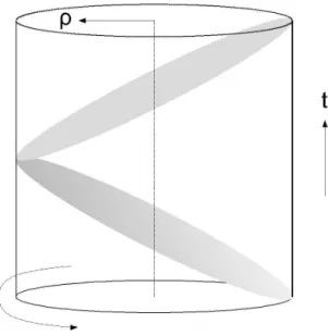
So far, most of the work that has been done in AdS/CFT was developed in the Poincar´e patch, but we have seen that Anti-de Sitter space is larger. Let us consider the case of AdS5. If we work on global coordinates we know that this
system covers all the space. The duality will tell us that gravity theory on this space will be equivalent to a CFT defined on its boundary, which in this case is the space R×S3 which is conformally related to R4, the boundary of Poincar´e
AdS.
Figure 7: Diagram of the conformal mapping
In global coordinates the metric of AdS5 can be written as:
ds2 = R
2
cos2θ(−dτ
2+dθ2+ sin2θdΩ2
3) (56)
And as we approach the boundary θ →π/2 we get:
ds2 = R
2
cos2θ(−dτ
2+dΩ2
3) (57)
On the other hand, in Poincar´e coordinates AdS metric:
So, we can write:
ds2 =f(x)dx2 =g(x)(dx′2+x′2dΩ3) =h(x)(
dx′2
x′2 +dΩ 2
3) (59)
finally,
5
Holography
By holography we mean the way to relate or encode whatever is happening in the bulk into information on the boundary. In this case the main tool is the bulk-to-boundary propagator. The first checks of the correspondence via n-point functions were originally done in Poincar´e coordinates with Euclidean signature, in this chapter we will follow this approach and later we will try to understand how the duality works in other coordinates. We will see that in this case, where we are calculating tree-level graphs in supergravity, the external legs of the graphs represent the boundary value of fieldsφ0 rather than asymptotic states as we were
used to in conventional Feynman diagrams.
The relation between mass m and scaling dimension ∆ for a vast kind of oper-ators/fields has been determined in several works, the majority has been done by calculating n-point functions in classical supergravity at tree level. Some of the results that we will check here are the following:
• Scalars: ∆± = 12 d±
√
d2+ 4m2
• Vectors: ∆±= 12
d±p
(d−2)2+ 4m2
• Spinors: ∆ = 1
2(d+ 2|m|)
• p-Forms: ∆± = 12
d±p
(d−2p)2+ 4m2
5.1
Holography for Scalar Fields
The prescription to calculate bulk-to-boundary propagators was proposed by Wit-ten and it has been applied in several cases to compute n−point functions for classical Supergravity in a AdS background. The results have been checked with the results coming from conformal invariance of some field theories.
The bulk-to-boundary propagator is defined as follows: If F(xa) is the
asymp-totic behavior dependence of some field φ(x) as xa →boundary, it means that
φ(x)xa→−→boundary F(xa)f(b) (61)
wherebrepresents the coordinates on the boundary, then the bulk-to-boundary propagator KB∂(b, x) is defined such that
φ(x) =
Z
Now, we are going to calculate the propagator for a massless scalar field in Eu-clidean Poincar´e coordinates by using Witten’s method, which exploits the sym-metries of AdS and its boundary. The equation of motion is given by
1
√ −g∂µ
√
−ggµν∂νφ(x)
= 0 (63)
The boundary of Euclidean Poincar´e AdSd+1 is Rd plus a point at infinity,
then let the boundary point ~x′ represent p at infinity, so K(x;p) = K(x
0, ~x;p).
The propagator must be invariant under AdS isometry group, and translation invariance dictates it cannot depend on~x:
∂0 √g∂0K∞(x0)
= 0 (64)
d dx0
x−0d+1 d dx0
K∞(x0)
= 0 (65)
Letting K∞(x0) = c(x0)p
d dx0
p(x0)p−d
= 0 (66)
then we should have p(p−d) = 0, which non-trivial solution is given by p=d. Now, the propagator must be a delta function at a point x on the boundary and it should vanish on the boundaryx0 for any~x, so let us map the pointpto the
origin~x′ = 0 with a coordinate transformation belonging to the isometry group:
xi −→
xi
x2
0+
P
x2 j
(67)
With this transformation the new propagator holds:
K(x0, ~x;p)−→K(x0, ~x;~0) =
c(x0)d
(x2
0+~x2)d
(68)
Then, from translation invariance on the boundary ~x→~x−~x′ we have:
K(x0, ~x;~x′) =
c(x0)d
(x2
0+ (~x−~x′)2)
d (69)
We can check that our propagator has the expected delta function behavior: For x0 → 0+ the propagator behaves as K ∼ δd(~x−~x′) and for ~x 6= ~x′ K → 0
as x0 →0, so the equation (69) represents the bulk-to-boundary propagator for a
Now, let us calculate the propagator for a massive scalar field. The equation of motion is given by:
1
√g∂α(√ggαβ∂β)−m2
φ(x) = 0 (70)
We find that a massive scalar of mass m in AdSd+1 couples to an operator O
in the boundary with ∆ = ∆+. ∆(∆−d) =m2
∆± =
d
2 ±
s
d
2
2
+m2 (71)
Again we look for a propagator vanishing at x0 = 0 but a delta function at
p: x0 =∞, it must be independent of ~x, so K(x;p) =K(x0, ~x;p) =K∞(x0) and
the equation of motion gives:
−xn+10 d dx0
x−0d+1 d dx0
+m2
K∞(x0) = 0 (72)
with the ansatz K∞(x0) =c(x0)λ+d we obtain
−(λ+d)λ+m2 = 0 (73) Then λ±= 12 −d±
√
d2+ 4m2
and the only solution which gives a vanishing propagator for x0 is λ+.
Taking into account d+λ+ =d−λ−= ∆+ and using the same isometry
prop-erties of the space as in the massless case we find the bulk-to-boundary propagator for the massive scalar field.
K(x0, ~x;~x′) =
c∗(x
0)∆+
(x2
0+ (~x−~x′)2)
∆+ (74)
To fix the constant c∗ we look at the asymptotic behavior of the propagator K
as x0 goes to zero. We find that K →c∗x∆0+ if ~x6=~x′ and K →c∗x
−∆+
0 if ~x=~x′.
Then K →c∗ǫ∆−δd(~x−~x′). We fix c∗ such that: 1 =R
ddxǫ−∆−K(ǫ, ~x; 0), then:
1 =
Z
ddxc
∗ǫ−∆−ǫ∆+
(ǫ2+~x2)∆+ =
ǫ∆+−∆−+d
ǫ2∆+ c
∗
Z
ddx 1
(1 +~x2)∆+ =c
∗ Γ(∆+)
πd/2Γ(∆
+−d/2)
(75) and finally:
K(x0, ~x;~x′) =
πd/2Γ(∆
+−d/2) (x0)∆+
5.2
n
-point functions for Scalar Fields
In the functional formulation of field theory we can calculate easily the n-point functions by using the generating functional or partition function. The boundary values φ0(x) of scalar fields serve as sources for operators O(x) of the conformal
field theory living on the boundary.
ZO[φ0] =
Z
D(f ields) exp
−SSY M+
Z
d4xO(x)φ0(x)
(77)
Then, by functional derivatives we can compute the n-point functions on the CFT:
hO(x1). . . O(xn)i=
δn
δφ0(x1). . . δφ0(xn)
ZO[φ0]|φ0 (78)
According to the AdS/CFT correspondence the partition function of the CFT is equivalent to the generating functional of a supergravity theory in AdS, so we can compute correlators from the gravity side and match them with results coming from the conformal invariance on the other side of the correspondence. In the AdS side we have:
Z[φ0] = exp (−Ssugra[φ[φ0(x)]]) (79)
Given a source scalar field living on the boundary φ0(~x) we can find its
“prop-agated field“ in the bulk through the bulk-to-boundary propagator found in the last section:
φ(~x, x0) =
Z
ddyKB∂(~x, x0;~y)φ0(~y) (80)
The idea is to find the classical solution φ[φ0] and replace it inSsugra.
Ssugra=
Z
dd+1x√g(∂µφ(~x, x0)∂µφ(~x, x0) +. . .) (81)
Then we can try to calculate the two-point function by using brute force:
hO(x1)O(x2)i= −
δ2S sugra
δφ0(x1)δφ0(x2)
φ0=0
(82)
We are taking two derivatives of φ0 and then making φ0 = 0, so we can neglect
hO(x1)O(x2)i= −
δ2
δφ0(x1)δφ0(x2)
Z
dd+1x√g∂µ
Z
ddyKB∂(~x, x0;~y)φ0(~y)
×∂µ
Z
ddy′KB∂(~x, x0;~y′)φ0(~y′)
=−
Z
dd+1x√g∂µKB∂(~x, x0;~x1)∂µKB∂(~x, x0;~x2)
(83)
That is the general approach one can use for a n-point function. To compute higher point functions we must keep non-linear terms and consider bulk-to-bulk propagators as well as bulk-to-boundary propagators.
Now let us calculate in a different and shorter way the 2-point function for the case of the scalar field. We take:
S = η 2
Z
dd+1x√g ∂µφ∂µφ+m2φ2
(84) Integrating by parts we get:
S = η 2
Z
dd+1x√gφ −∇φ+m2φ2
+η 2
Z
dd+1x√gφ∂µ(φ∂µφ) (85)
The remaining term vanish everywhere except in the x0 direction where we
have the boundary. Then, we evaluate at the boundary x0 =ǫ:
S = η 2
Z
∂
ddx√hφ~n·∇~φ (86)
We have √h=x−0d and~n·∇~φ =x0∂x∂0φ. Also limǫ→0φ(~x, x0) =φ0(~x)
Then, we obtain:
x0
∂ ∂x0
φ=x0
∂ ∂x0
Z
d4x′KB∂(~x, x0;~x′)φ0(~x′) (87)
As x0 goes to zero, we get:
x0
∂ ∂x0
φ=c∗∆×x0x∆0−1
Z
d4x′ φ0(~x
′)
(~x−~x′)2∆ (88)
And so:
S = η 2limǫ→0
Z
ddxddx′ǫ∆−dc∗∆× φǫ(~x)φ0(~x
′)
(~x−~x′)2∆ (89)
hO(x1)O(x2)i=−
c∗η∆
2 × 1
|~x−~x′|2∆ (90)
In this treatment φ0 must be a small perturbation around a CFT, otherwise
there is going to be a backreaction on the geometry. This is required in order to use perturbation theory.
A general action for scalar field in d+ 1 dimension is given by:
I[φ] =
Z
Ω
dd+1x√−g
"
1 2
(∇φ)2+m2φ2
+X
n≥3
λn
n!φ
n
#
(91)
The equation of motion is then:
∇2−m2
φ=X
n≥3
λn
(n−1)!φ
n−1 (92)
And so the covariant Green’s function will satisfy:
∇2−m2
G(x, y) = δ(x, y) = √1
−gδ(x−y) (93)
and the boundary condition G(x, y)|x∈∂Ω. The formal solution is:
φ(x) =
Z
∂Ω
ddy√hηµ∂µ,yG(x, y)φ(y) +
Z
Ω
dd+1y√gG(x, y)X
n≥3
λn
(n−1)!φ
n−1(y)
(94) For the n-point functions (n ≥3) at tree level we will only have contributions from the interaction term in the action:
I[φ] =X
n≥3
λn
n!
Z
Ω
dd+1x√g φ(0)n
(95)
It turns out that at tree-level one can take the limit ǫ→0 beforehand and so:
I1[φ] =X
n≥3
λn
n!
Z
Ω
dd+1x√g c∗
Z
ddyφ(~y)
x0
x2
0+|~x−~y|2
∆!n
(96)
where √g = (x0)d+1.
I1[φ] =X
n≥3
cnλ n
n!
Z
ddy1ddy2· · ·ddynφ(~y1)· · ·φ(~yn)
×
Z
dd+1x (x0)n∆−(d+1)
[(x2
0+|~x−~y1|2)· · ·(x20+|~x−~yn|2)]∆
Figure 8: Witten diagram for 3-point function at tree level
Calling:
In(x1,· · · , xn) =
Z
dd+1x (x0)
n∆−(d+1)
[(x2
0+|~x−~y1|2)· · ·(x20+|~x−~yn|2)]∆
(98) The connected part of the tree-level n-point functions is given by:
hφ(x1)· · ·φ(xn)i=−λncnIn(x1,· · · , xn) (99)
The task is to evaluate the integral In. We need the useful formula so-called
Feynman parameterization:
1
Aα1
1 · · ·Aαnn
= Γ(
P
αi)
Q
iΓ(αi)
Z
du1. . . dun
δ(P
uk−1)uα11−1. . . uαnn−1
(u1A1+· · ·+unAn)
P
αk (100)
Then, we can rewrite In as:
In=
Γ(n∆) Γn(∆)
Z
du1. . . dunδ(
X
uk−1)
Y
u∆i −1
Z
dd+1x (x0)
n∆−(d+1)
[P
iui(x20 + (~x−~yi)2)]n∆
(101) We will useP
iui = 1 as well as the volume of the unitary d-dimensional sphere
Ωd= 2π
d/2
Γ(d/2) and:
Z ∞
0
dk k
l−1
(k2+v2)m = (v
2)l/2−mΓ(l/2)Γ(m−l/2)
2Γ(m) (102) Integrating the x0 variable: l=n∆−d, m=n∆
In=
Γ(n∆)Γ(n∆
2 − d 2)Γ( n∆ 2 + d 2)
2Γ(n∆)Γn(∆)
Z
duiδ(
X
uk−1)
Y
u∆i −1
Z
ddx 1
[P
iui(~x−~yi)2]
n∆ 2 +
d
Calling:
Ii =
Z
ddx 1
[P
iui(~x−~yi)2]
n∆ 2 + d 2 = Z
ddx 1
[x2−2P
iui~x·~yi+
P
iui~yi2]
n∆ 2 + d 2 = Z
ddx 1
[x2−2P
iui~x·~yi+ (
P
iui~yi)2−(
P
iui~yi)2 +
P
iui~y2i]
n∆ 2 +d2
(104)
changing variables~x →~x+P
iui~yi:
Ii =
Z
ddx 1
[x2+P
iui~yi2−(
P
iui~yi)2]
n∆ 2 +
d
2
= ΩdΓ(
n∆
2 )Γ(
d 2)
2Γ(n∆2 +d2) ×
1 [P
iui~yi2−(
P
iui~yi)2]
n∆ 2
(105)
and we can rewrite the denominator as:
X
i
ui~yi2−(
X
i
ui~yi)2 =
X
i,j
uiuj~yi2−
X
i,j
uiuj~yi·~yj
= 1 2
X
i,j
uiuj(~yi−~yj)2
=X
i<j
uiuj(~yi−~yj)2
(106)
So back in In we have:
In =
πd/2Γ(n∆
2 −
d
2)Γ(
n∆
2 )
2Γn(∆)
Z
dui
δ(P
uk−1)Qu∆i −1
h P
i<juiujr2ij
in2∆ (107)
We can make ui →β1βi and β1 =u1:
In =
πd/2Γ(n∆
2 −
d
2)Γ(
n∆
2 )
2Γn(∆)
Z ∞
0
dβ2. . . dβn
Qn
i=2β ∆−1 i
h P
i=2βi(r1i2 +
P
j>1βjrij2)
in2∆ (108)
hφ(x1)φ(x2)φ(x3)i= −
c3λ 3
2 I3(x1, x2, x3) (109) Notice that without our reduced formula, the first diagram calculation will be:
hφ(x1)φ(x2)φ(x3)i=
Z
ddzλ3KB∂(x1, z)KB∂(x2, z)KB∂(x3, z) (110)
But now we have a simpler calculation starting from
hφ(x1)φ(x2)φ(x3)i= −
c3λ 3
2
πd/2Γ(3∆
2 −
d
2)Γ(
3∆
2 )
2Γ3(∆)
Z ∞
0
dβ2dβ3
β2∆−1β3∆−1
[β2r122 +β2β3r232 +β3r132 ]
3∆ 2
(111) To perform this integral we need:
Z ∞
0
xmdx
(a+bx)n+1/2 = 2
m+1m!(2n−2m−3)!!
(2n−1)!!
am−n+1/2
bm+1 (112)
and calling:
Iβ =
Z ∞
0
dβ2dβ3
β2∆−1β3∆−1
[β2r212+β2β3r223+β3r213)]
3∆ 2
= 2
∆Γ(∆)(∆−2)!!
(3∆−2)!!
Z ∞
0
dβ3
β3∆/2−1
r∆
13(r212+β3r223) ∆
(113)
Then:
Iβ =
23∆/2Γ(∆)Γ(∆/2)(∆−2)!!(∆−2)!!
(3∆−2)!!(2∆−2)!!
1 (r13r12r23)∆
(114)
And taking into account (2k)!! =k!2k and c= Γ(∆)
πd/2Γ(∆−d/2) we finally find:
hφ(x1)φ(x2)φ(x3)i= −
λ3Γ3(∆/2)
2πd(r
13r12r23)∆
Γ(3∆
2 −
d
2)Γ(3∆/2)Γ
3(∆)
Γ3(∆−d/2)Γ3(∆)Γ(3∆/2) (115)
We can rewrite the result with α = ∆−d/2:
hφ(x1)φ(x2)φ(x3)i= −
λ3Γ(∆2 +α)
2πd
"
Γ(∆2) Γ(α)
#3
1 (r13r12r23)∆
(116)
in-dynamics in this case depends on the conformal dimension of the scalar field. We can also have terms of the kind φ∂φ∂φ and we will obtain contributions with the same functional form and different coefficient.
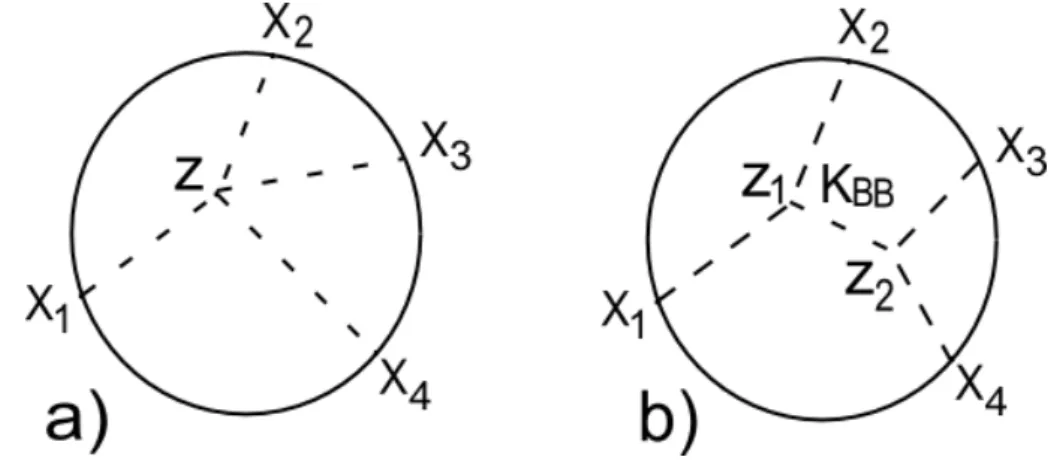
Now, let us calculate the 4-point function at tree level, in this case we have 2 diagrams with the same order:
Figure 9: Witten diagrams for 4-point function at tree level
Again, if we were to calculate by brute force the first diagram (partaof Figure 9):
hφ(x1)φ(x2)φ(x3)φ(x4)iF irst diagram =
Z
ddzλ4KB∂(x1, z)KB∂(x2, z)KB∂(x3, z)KB∂(x4, z)
(117) The other contribution corresponding to the second diagram (part b) will have the form:
hφ(x1)φ(x2)φ(x3)φ(x4)iSecond diagram =
Z
ddz1ddz2(λ3)2 KB∂(x1, z1)KB∂(x2, z1)
×KBB(z1, z2)KB∂(x3, z2)KB∂(x4, z2)
(118) Here we will only calculate the first contribution. So, by using the previous results we obtain:
hφ(x1)φ(x2)φ(x3)φ(x4)i= −
c4λ 4
hφ(x1)φ(x2)φ(x3)φ(x4)iF irst diagram = −
c4λ 4
2
πd/2Γ(2∆− d
2)Γ(2∆)
2Γ4(∆)
×
Z ∞
0
dβ2dβ3dβ4
β∆−1
2 β3∆−1β4∆−1
[β2r122 +β3r132 +β4r142 +β2β3r232 +β2β4r242 +β3β4r342 ] 2∆
(120)
First, we proceed to calculate the integral over β4:
I4 =k
Z ∞
0
dβ2dβ3dβ4
β2∆−1β3∆−1β4∆−1
[β2r212+β3r213+β4r214+β2β3r223+β2β4r224+β3β4r234] 2∆
=k∆!(∆−3/2)!
(2∆−3/2)!
Z ∞
0
dβ2dβ3
β2∆−1β3∆−1
[(β2r122 +β3r132 +β2β3r232 )(r142 +β2r242 +β3r342 )] ∆
(121) This last integral has the form (page 314 in [22]):
Z ∞
0
xν−1(α+x)−µ(γ+x)−ρdx=α−µγν−ρB(ν, µ−ν+ρ)2F1(µ, ν;µ+ρ; 1−
γ
α) (122)
Taking α = β2r212
(r2
13+β2r232 ) and γ =
(r2
14+β2r242 )
r2
34 , µ=ν = ρ= ∆ we can perform the
integral and it holds:
I4 =k
∆!(∆−3/2)! (2∆−3/2)!
B(∆,∆)
r2∆ 12r2∆34
Z ∞
0
dβ2
β2 2
F1
∆,∆; 2∆; 1− (r
2
14+β2r242 )(r132 +β2r232 )
β2r212r342
(123) As we want to compare the calculations with the results form conformal invari-ant theories, we can rewrite the last result in terms of the harmonic ratios:
Taking:
η= r12r34
r14r23
(124)
ζ = r12r34
r13r24
(125)
β2 =
r13r14
r23r24
e2z (126)
We get dβ2
So
ηζ
(r12r34)
Y
i<j
rij = (r12r34)2 (127)
Then we can write:
I4 =k
∆!(∆−3/2)! (2∆−3/2)!
2B(∆,∆) (ηζQ
i<jrij)2∆/3
×
Z ∞
0
dz 2F1
∆,∆; 2∆; 1− (η+ζ)
2
(ηζ)2 −
4
ηζ sinh
2z
(128)
5.3
Holography for Gauge Fields
In general, if the theory in AdS has a gauge group G with gauge fields Aa, a =
1, . . . , k with k the dimension of the group, then according to the correspondence the symmetry associated is equivalent to a global symmetry of the Conformal theory on the boundary that acts on currents Ja. Along this subsection we will
use the notation introduced by Witten in [2]. For some fixed a we can call Aa
0 the value on the boundary of some field Aa
living in AdS, the conjecture states that it is source of some Ja on the boundary
and then according to the previous definitions, the prescription is given by:
ZS(Aa0) =
exp(
Z
∂AdS
JaAa0)
CF T
(129)
We will consider a field Aµ(x) belonging to a free U(1) gauge theory and look
for a solutions of equations of motion for the bulk-to-bulk propagator in AdS space, the simpler one with a singularity at only one point in the boundary, it means a delta function source. We write the classical action for the gauge field with a AdS background in Poincar´e coordinates:
I[A] =
Z
dd+1x√−g
−12FµνFµν
(130)
Then taking into account Fµν =∂µAν −∂νAµ we find the equation of motion
for the gauge field:
1
√ −g∂µ
√
−gFµν
= 0 (131)
In a similar way, we consider the single point p=∞at the boundary(x′
0 = 0)
representing ~x′ and so we expect a propagator independent of~x because of
trans-lation invariance. ThenA(x;x′) = A(x;p) = A(x
0, ~x;p) and we look for a solution
by a 1-form A =f(x0)dxi, where i is a fixed component(i ≥1). The ansatz must
satisfy the equation of motion and so: F0i = ∂x∂f0 →F0i =g0kgilFkl = (x0)4∂x∂f0 and
considering√−g = (x0)−d−1 (we are inAdSd+1) we obtain the equation of motion:
d dx0
[√gF0i] = d
dx0
[(x0)−d+3
∂f ∂x0
] = 0 (132) Then the quantity inside the brackets [ ] must be independent of x0 and we
obtain up to a constant factor ∂x∂f
0 = (x0)
d−3 or f(x
0) = (x0)d−2 and we can write
A= d−1
d−2(x0)
d−2dxi (133)
With the same arguments used in the scalar case the we must show that the singularity of the new solution at the infinity is a delta function. As we did before we map the point p to the origin~x′ = 0 with the inversionxi →xi/(x20+~x2) and
then the propagator takes the form:
A= d−1
d−2
x0
x2
0+~x2
d−2
d
xi
x2
0+~x2
(134) Despite the fact that it does not look like an usual propagator, we must remem-ber that it is “propagating” a delta source on the boundary, simply A(x0, ~x;~0) =
R
d~x′A(x
0, ~x;~x′)δ(~x′) from ~x′ = 0 on the boundary to (x0, ~x) in the bulk. To
sim-plify the calculations we can make use of the gauge invariance of the theory and subtract from the propagator the exterior derivative of
1
d−2
xixd0−2
(x2
0+~x2)d−1
(135) This is possible since δA = dΛ represents a gauge transformation. In this gauge we evade working with a propagator with components in all directions. The results we are to present have been obtained in another gauge choices. The new propagator is:
A= 1
d−2
"
(d−1)
x0
x2
0+~x2
d−2
dxi
x2
0+~x2
+ (d−1)
x0
x2 0+~x2
d−2
xid
1
x2
0+~x2
−d
xixd−2 0
(x2
0+~x2)d−1
(136)
A= 1
d−2
(d−1) x
d−2
0 dxi
(x2
0+~x2)d−1
+xixd0−2d
1 (x2
0+~x2)d−1
−d
xixd−2 0
(x2
0+~x2)d−1
(137)
A(x0, ~x;~0) =
1
d−2
(d−1) x
d−2
0 dxi
(x2
0+~x2)d−1
− x
d−2
0 dxi
(x2
0 +~x2)d−1
−(d−2) x
d−3
0 xidx0
(x2
0 +~x2)d−1
= x
d−2
0 dxi
(x2
0+~x2)d−1
− x
d−3
0 xidx0
(x2
0+~x2)d−1
(138) We wanted a solution such that on the boundary (x0 = 0) we have A0 =
P
aidxi and we can check this behavior in our previous result. First, we use
translation invariance in the bulk~x →(~x−~x′) and we can write for an arbitrary
source on the boundaryai(~x′):
A(x0, ~x) =
Z
ddx′A(x0, ~x;~x′)ai(~x′)
=xd0−2
Z
ddx′
ai(~x′)dxi
(x2
0+ (~x−~x′)2)d−1
−xd0−3dx0
Z
ddx′
ai(~x′)(x−x′)i
(x2
0+ (~x−~x′)2)d−1
(139) The first term is a delta function as x0 goes to zero and the second vanishes.
Now we can calculate the field strength F =dA= (dx0∂0+dxi∂i)A:
F = (d−2)xd0−3dx0∧
Z
ddx′
ai(~x′)dxi
(x2
0+ (~x−~x′)2)d−1
−2(d−1)xd0−1dx0∧
Z
ddx′
ai(~x′)dxi
(x2
0+ (~x−~x′)2)d
+2(d−1)xd0−3dxj∧dx0
Z
ddx′
ai(~x′)(x−x′)j(x−x′)i
(x2
0+ (~x−~x′)2)d
−xd0−3dxi∧dx0
Z
ddx′
ai(~x′)
(x2
0+ (~x−~x′)2)d−1
+. . .
(140)
where the dots indicate terms with no dx0.
In form language we can rewrite the classical action by using F =dA and the equation of motion d ⋆ F = 0:
I[A] = 1 2
Z
AdSn+1
F ∧⋆F = 1 2
Z
AdSn+1
d(A∧⋆F) (141)
and this will not vanish only in x0 = 0 where we have the boundary of AdS
space:
Now we see the reason we forgot about the terms with nodx0 in the calculation
of the field strength: We only need the componentsi= 1, . . . , dof (A∧⋆F) and ac-cording with the definition of the⋆operation: ⋆Tµ1...µp = 1
(D−p)!ǫ
µ1µ2...µd+1T
µp+1...µd+1
for aicomponent ofAthen⋆F has no 0 or thaticomponent. So we need only the 0i components of F and our action will take the form (note 1/2 factor disappear because of F0i =−Fi0):
I[A] = 1 (d−1)
Z
ddx√h(n0AjF0j) (143)
where the (d−1) factor appears from (D−p) = (d+ 1−2), n0 is the zero
component of a unit vector normal (gµνnµnν = 1) to the boundary which we can
define it as nµ = (x
0, . . . ,0) and the hij is the “residual” metric in the boundary
of the AdS space which holds:
hij =
1
x2 0
δij (144)
The boundary is d−dimensional, therefore √h = x0−d. Using dx0 ∧ dxi =
−dxi∧dx0 we can rewrite the field strength:
F = (d−1)xd0−3dx0∧
Z
ddx′
ai(~x′)dxi
(x2
0+ (~x−~x′)2)d−1
−2(d−1)xd−1
0 dx0∧
Z
ddx′
ai(~x′)dxi
(x2
0+ (~x−~x′)2)d
−2(d−1)xd0−3dx0∧
Z
ddx′
ai(~x′)(x−x′)j(x−x′)idxj
(x2
0+ (~x−~x′)2)d
+. . .
(145)
Now
I[A] = 1 (d−1)
Z
ddx x−0d[x0hijAi(x0, ~x)F0j(x0, ~x)]
= 1 (d−1)
Z
ddx x−0d+3[δijAi(x0, ~x)F0j(x0, ~x)]
(146)
Taking the limit x0 →0 the leading term in F will be x0d−3 and Ai →ai(~x):
I[A] = 1 (d−1)
Z
ddx ddx′δij
(d−1)
Ai(x0, ~x)aj(~x′)
(x2
0+ (~x−~x′)2)d−1
−2(d−1)
Ai(x0, ~x)(x−x′)jak(~x′)(x−x′)k
(x2
0+ (~x−~x′)2)d
I[A] =
Z
ddx ddx′ a
i(~x)aj(~x′)
δij
(~x−~x′)2d−2 −
2(x−x′)i(x−x′)j
(~x−~x′)2d
(148)
And so the 2-point function is given by:
Ji(~x)Jj(~x′)
= 1
(~x−~x′)2d−2
δij −2(x−x
′)i(x−x′)j
(~x−~x′)2
(149)
We check that this result has the form:
Ji(~x)Jj(~x′)
= 1 (~x−~x′)2∆R
ij(~x, ~x′)
(150)
where we can identify the scaling dimension of this gauge field ∆ =d−1 and we also obtain the vectorial representation matrix Rij(~x, ~x′):
Rij(~x, ~x′) = δij − 2(x−x
′)i(x−x′)j
5.4
Holography for Spinor Fields
The case of spinor fields is a bit more involved because the free action vanishes on-shell and so we have to supplement it with surface terms on the boundary. This fact is known for fields satisfying first order equations of motion and in order to make sense of 2-point function for these fields within AdS/CFT correspondence, the inclusion of boundary terms was the proposed solution and people have worked on some other cases by using the same procedure. Besides, as we need to couple the background with the spinor field we must use the formalism of vielbein and spin connection.
We will write the action as:
I[ψ] =
Z
AdS
dd+1x√g ψ¯(6D−m)ψ+k
Z
∂AdS
ddx √hψψ¯ (152) The relative parameterkwill be fixed by the theory we are defining in theAdS
space. It can depend, for instance, on gauge invariance or supersymmetry.
As we mentioned, we have to choose a local Lorentz frame, it means gµν =
ea
µebνηab, and considering the metric of AdS space in Poincar´e coordinates the
nat-ural choice of the vielbein is:
eaµ = δ
a µ
x0
(153) and we can define the spin connection as:
ωi0j =−ωij0 = δ
j i
x0
(154) Then, the slashed covariant derivative is given by:
6
D= Γµ
∂µ+
1 4ω
ab µ Γab
=eµaΓa
∂µ+
1 4ω
bc µΓbc
=x0Γ0∂0+x0~Γ· ∇+
1 2x0δ
i aΓaω
0j i Γ0j
=x0Γ0∂0+x0~Γ· ∇+
1 2δ
i aδ
j
iΓaΓ0j =x0Γ0∂0+x0~Γ· ∇+
1 2Γ
jΓ 0j
=x0Γ0∂0+x0~Γ· ∇ −
d
2Γ
0
(155)
Where we have used Γab = 12[Γa,Γb] and{Γa,Γb}= 2ηab.
Now we can try to solve the equation of motion for the propagator by using the same considerations that we have used in the previous cases. Let us call
so it does not depend on the value of~x′ and ~xbecause of translation invariance in
the bulk. So our ansatz should depend only on x0. Then we propose G∞(x0) =
f(x0)x0Γ0 so
(−x0∂0+
d
2−mΓ
0)G
∞(x0) = 0 (156)
gives G∞(x0) = (x0)
d
2−mΓ0Γ0.
Now we can bring the point p=∞ to an arbitrary finite point on the bound-ary by the isometry group transformation xi → xi/(x20 +~x2), but this has to be
accompanied by a local Lorentz transformation ea
µ = Λabebµ to preserve the choice
of the vielbein.
Instead of the same strategy to find the boundary-to-bulk propagator we will show another method developed on [23] based on the transformation property of the Dirac operator under inversion.
First we must find an operator U(x) which will represent the inversion that will transform the vectorial index in the spinorial representation, it is:
U−1(x)ΓµU(x) =−Jµν(x)Γν (157)
where Jµν(x) is the jacobian of the operation. To see this let us consider the
inversion ˆxµ=xµ/x2, then we find
∂xˆµ
∂xν
= 1
x2(δµν −2
xµxν
x2 ) =
1
x2Jµν(x) (158)
also
∂ ∂xν
= 1
x2Jµν(x)
∂ ∂xˆν
(159)
Jµν(x)Jνα(x) =Jµα(x) (160)
The solution is given by
U(x) = Γ
µx µ
√x
0
(161)
ΓµU(x) = (−ΓνΓµ+ 2δµν)
xν
√x
0
= √2xµ
x0 −
U(x)Γµ
= √2xµ
x0x2
δαβxαxβ−U(x)Γµ
= √2xµ
x0x2
ΓαΓβxαxβ−U(x)Γµ=−U(x)(Γµ−
2xµ
x2 Γαx α)
=−U(x)Jµν(x)Γν
(162)
Finally we get:
U−1(x)ΓµU(x) =−Jµν(x)Γν (163)
And we will derive another property:
DµU(x) =x0∂µ(
Γνx ν
√x
0
) = Γ√µX0
x0 −
U(x)δµ0
2 = Γ√µx0
x0 −
ΓµΓ0U(x)
2 = Γµx0
√x
0 −
ΓµΓ0Γ0x0
2√x0 −
ΓµΓ0Γixi
2√x0
= 1
2ΓµU(x)Γ0
(164)
From these it is straightforward to obtain the inversion of the Dirac operator:
6
D(ˆx) =U−1(x)6D(x)U(x) + 1
2Γ0 (165) Now, we must remember that we are looking for a propagator which is a solution of (6D(x)−m)Σ = 0 and rewriting the last result we obtain:
−U(x)[6D(ˆx) +m− 1
2Γ0]U
−1(x) =6D(x)−m (166)
Finally it is easy to see the solution for the bulk-to-boundary propagator:
Σ(x) =U(x)ˆx
d+1 2 −mΓ0
0 = (x0Γ0+~x·Γ)(~ x20+~x2)mΓ0−
d+1 2 x
d
2−mΓ0
0 (167)
Then after using translation invariance we find:
ψ(x0, ~x) =
Z
ddx′x
0Γ0+ (~x−~x′)·~Γ
x2
0+ (~x−~x′)2
mΓ0−d+12
x−0mΓ0+d/2ψ0(~x′)
and similarly
¯
ψ(x0, ~x) =
Z
ddx′ψ¯0(~x′)xmΓ
0+d/2
0 x20+ (~x−~x′)2
−mΓ0−d+12
x0Γ0 + (~x−~x′)·~Γ
(169) Now we must determine and “choose” the behavior of the solutions near the boundary. By calling Γ0ψ
±(~x′) = ±ψ±(~x′) and ¯ψ±(~x′)Γ0 = ±ψ¯±(~x′), we
decom-pose the solutions:
lim
x0→0
(x0)m−
d
2ψ(x
0, ~x) =−kψ−(~x) +
Z
ddx′|~x−~x′|2m−d−1~Γ·(~x−~x′)ψ
+(~x′) (170)
lim
x0→0
(x0)m−
d
2ψ¯(x
0, ~x) =kψ¯+(~x) +
Z
ddx′ψ¯−(~x′)|~x−~x′|2m−d−1~Γ·(~x−~x′) (171)
Now, we must impose boundary conditions on the solutions. Notice from the first order differential equation that we are solving, half the components can be fixed. In general, there is not a natural choice of these components, but it has been shown that ψ+(~x′) = 0 and ¯ψ−(~x′) = 0 seem to work .
Now, replacing the results in the surface term added the action we find:
Z[ψ] =e−I1 = exp
−lim
ǫ→0
Z
ddx√Σ ¯ψψ
= exp
−lim
ǫ→0
Z
ddx
Z
ddx′
Z
ddx′′ǫ−dǫm+d/2 ǫ2+ (~x−~x′′)2−m−d+12
×(~x−~x′′)·~Γ ǫ2 + (~x−~x′)2−m−d+12
ǫm+d/2+1
= exp
−
Z
ddx′
Z
ddx′′ ψ¯+(~x′)D(~x′, ~x′′)ψ−(~x′′)
(172) where we identify D(~x′, ~x) with the 2-point function:
D(~x′′, ~x′) = lim
ǫ→0
Z
ddxǫ2m+1
ǫ2+|~x′′−~x|2−m−d+12
(~x′′−~x′)·Γ
ǫ2 +|~x′−~x|2−m−d+12
(173) and so:
D(~x′′, ~x′) =k (~x
′′−~x′)·Γ
|~x′′−~x′|2m+d+1 =k
(~x′′−~x′)·Γ
|~x′′−~x′|
1
|~x′′−~x′|2(m+d/2)
Then the 2-point function for a primary spinor operator Oα with scaling
di-mension ∆ =m+d/2 is given by
Oβ(~x′′)Oα(~x′)
=k(~x
′′−~x′)·(Γ)βα
|~x′′−~x′|
1
|~x′′−~x′|2∆ (175)


![Figure 8: Witten diagram for 3-point function at tree level Calling: I n (x 1 , · · · , x n ) = Z d d+1 x (x 0 ) n∆−(d+1) [(x 2 0 + |~x − ~y 1 | 2 ) · · · (x 20 + |~x − ~y n | 2 )] ∆ (98) The connected part of the tree-level n-point functions is given by:](https://thumb-eu.123doks.com/thumbv2/123dok_br/15750196.126831/34.892.328.562.122.350/figure-witten-diagram-function-level-calling-connected-functions.webp)