❊♥s❛✐♦s ❊❝♦♥ô♠✐❝♦s
❊s❝♦❧❛ ❞❡
Pós✲●r❛❞✉❛çã♦
❡♠ ❊❝♦♥♦♠✐❛
❞❛ ❋✉♥❞❛çã♦
●❡t✉❧✐♦ ❱❛r❣❛s
◆◦ ✸✻✻ ■❙❙◆ ✵✶✵✹✲✽✾✶✵
❋♦r❡✐❣♥ ❉✐r❡❝t ■♥✈❡st♠❡♥t ❙♣✐❧❧♦✈❡rs✿ ❲❤❛t
❈❛♥ ❲❡ ▲❡❛r♥ ❋r♦♠ P♦rt✉❣✉❡s❡ ❉❛t❛❄
▼❛r✐❛ P❛✉❧❛ ❋♦♥t♦✉r❛✱ ❘❡♥❛t♦ ●❛❧✈ã♦ ❋❧ôr❡s ❏✉♥✐♦r✱ ❘♦❣ér✐♦ ●✉❡rr❛ ❙❛♥t♦s
❏❛♥❡✐r♦ ❞❡ ✷✵✵✵
♦♣✐♥✐õ❡s ♥❡❧❡s ❡♠✐t✐❞❛s ♥ã♦ ❡①♣r✐♠❡♠✱ ♥❡❝❡ss❛r✐❛♠❡♥t❡✱ ♦ ♣♦♥t♦ ❞❡ ✈✐st❛ ❞❛
❋✉♥❞❛çã♦ ●❡t✉❧✐♦ ❱❛r❣❛s✳
❊❙❈❖▲❆ ❉❊ PÓ❙✲●❘❆❉❯❆➬➹❖ ❊▼ ❊❈❖◆❖▼■❆ ❉✐r❡t♦r ●❡r❛❧✿ ❘❡♥❛t♦ ❋r❛❣❡❧❧✐ ❈❛r❞♦s♦
❉✐r❡t♦r ❞❡ ❊♥s✐♥♦✿ ▲✉✐s ❍❡♥r✐q✉❡ ❇❡rt♦❧✐♥♦ ❇r❛✐❞♦ ❉✐r❡t♦r ❞❡ P❡sq✉✐s❛✿ ❏♦ã♦ ❱✐❝t♦r ■ss❧❡r
❉✐r❡t♦r ❞❡ P✉❜❧✐❝❛çõ❡s ❈✐❡♥tí✜❝❛s✿ ❘✐❝❛r❞♦ ❞❡ ❖❧✐✈❡✐r❛ ❈❛✈❛❧❝❛♥t✐
P❛✉❧❛ ❋♦♥t♦✉r❛✱ ▼❛r✐❛
❋♦r❡✐❣♥ ❉✐r❡❝t ■♥✈❡st♠❡♥t ❙♣✐❧❧♦✈❡rs✿ ❲❤❛t ❈❛♥ ❲❡ ▲❡❛r♥ ❋r♦♠ P♦rt✉❣✉❡s❡ ❉❛t❛❄✴ ▼❛r✐❛ P❛✉❧❛ ❋♦♥t♦✉r❛✱
❘❡♥❛t♦ ●❛❧✈ã♦ ❋❧ôr❡s ❏✉♥✐♦r✱ ❘♦❣ér✐♦ ●✉❡rr❛ ❙❛♥t♦s ✕ ❘✐♦ ❞❡ ❏❛♥❡✐r♦ ✿ ❋●❱✱❊P●❊✱ ✷✵✶✵
✭❊♥s❛✐♦s ❊❝♦♥ô♠✐❝♦s❀ ✸✻✻✮
■♥❝❧✉✐ ❜✐❜❧✐♦❣r❛❢✐❛✳
Foreign direct investment spillovers: what can we learn from
Portuguese data ?
1Renato G. Flôres Jr.* , Maria Paula Fontoura** and Rogério Guerra Santos**
* EPGE / Fundação Getúlio Vargas, Rio de Janeiro ** ISEG / Universidade Técnica de Lisboa, Lisbon
Abstract
This paper investigates the impact of foreign direct investment on the productivity performance of domestic firms in Portugal. The data comprise nine manufacturing sectors for the period 1992-95. Relatively to previous studies, model specification is improved by taking into consideration several aspects: the influence of the “technological gap” on spill-overs diffusion and the choice of its most appropriate interval; sectoral variation in the coefficients of the spill-overs effect; identification of constant, idiosyncratic sectoral factors by means of a fixed effects model; and the search for inter-sectoral positive spillover effects. The relationship between domestic firms productivity and the foreign presence does take place in a positive way, only if a proper technology differential between the foreign and domestic producers exists and the sectoral characteristics are favourable. In broad terms, spillovers diffusion is associated to modern industries in which the foreign owned establishments have a clear, but not too sharp, edge on the domestic ones. Besides, other specific sectoral influences can be pertinent; agglomerative location factors being one example.
JEL Codes: F14, O52
Keywords: domestic firm productivity; foreign direct investment; Portugal; technological spillovers.
(This version: January, 2000)
1
1. INTRODUCTION
One benefit often cited in the literature on the gains from foreign direct investment (FDI), apart from the capital inflows and additional employment, is the increase in domestic firms´ productivity. This is related to the concept of technology or
productivity spillovers, which embodies the fact that foreign enterprises own intangible assets such as technological know-how, marketing and managerial skills, international experience or reputation, which can be transmitted to domestic firms, raising their productivity level. Spillovers diffusion is thus a matter of externalities within the country, from established foreign producers to domestic ones, and can be associated to two group of effects: knowledge spillovers and competitive disciplinary effects. The former are mainly (i) new technology either embodied in imported inputs and capital goods, or sold directly through licence agreements, or transferred to domestic producers who learn new techniques from their foreign buyers; (ii) learning by doing among domestic firms combined with investments in formal education and on-the-job training of domestic employees who move from foreign to domestic firms; (iii) cost savings due to technology passed to downstream users of new products or upstream buyers or suppliers. The latter are associated to “incentives” to competition among domestic firms, resulting from the foreign affiliates entrance, through either a more efficient use of existing technology and resources or a search for more efficient technologies, or a restraint on the exercise of market power by domestic firms.
It is because the spillover concept has a broader meaning than imitation or even technology diffusion that it can be primarily associated to productivity. However, on what concerns the “knowledge effect”, it is inherently an abstract concept, which comprises not only knowledge and skills but also “the means for using and controlling factors of production” (Kokko, 1992. p. 21), such as product, process, distribution technology or management skills2.
Empirical evidence on spillovers diffusion is ambiguous. Using sectoral data, Blomström (1986) found that an increase in foreign presence fails to increase the productivity growth of domestic firms. Santos (1991) also did not find a positive influence on the productivity level for the case of Portugal, in the period 1977-82.
2
Conversely, Blomström and Persson (1983) and Blomström and Wolff (1994) found that domestic labour productivity is positively influenced by foreign presence.
Micro-econometric studies with panel data sets of entreprises are in general more supportive of a negative influence, though a positive effect of FDI on the productivity of domestic firms was found by Farinha and Mata (1996) in Portugal, with an analysis at the firm level, covering the 1986-92 period. Haddad and Harrison (1993), Harrison (1996) and Aitken and Harrison (1997) found a negative significant relationship between the size of foreign presence and the productivity performance of domestic firms. In Djankov and Hoekman (1999) there is also a statistically significant negative spillover effect of foreign participation in an industry, through joint ventures and FDI, as regards Czech firms without such links.
The case study literature, on the other hand, seems to point more clearly to positive spillovers. This leads us to suspect that econometric results can be somehow related to a specification problem. Indeed, the present state of the theory does not allow to build proper dynamic, structural models of spillovers´ impact on the productivity of domestic enterprises. The negative results might thus be related to omitted variables and the reduced form used.
This paper investigates the impact of foreign investment on the productivity performance of Portuguese firms. When Portugal joined the European Union in 1986, foreign direct investment as a percentage of GDP had never passed the 1% threshold. After 1988, this ratio reached a maximum peak of 4% in 1990 and, though it has continuously decreased since then, it has never crossed back the 1% line3. This obviously raises interest on the indirect effects of FDI in the country.
The study is conducted for the manufacturing sector at the two-digit level. Data restrictions limited us to nine groups (or sectors), for the period 1992-95; however, the panel nature of the data allows to go beyond cross-section analysis and use some techniques particularly appropriate to exploit the sector specifities.
We worked with six successive models. Relatively to previous studies, we improved on model specification by not only including variables which control for other productivity shocks but, especially, by searching the most appropriate interval on what concerns the influence of the “technological gap” on spillovers diffusion. Sectoral variation in the parameters of the spillovers effect, and the identification of constant but
3
specific (idiosyncratic) sectoral factors were also tested. Finally, we tried to identify, in an exploratory way, inter-sectoral positive spillover effects.
In what follows, section 2 presents the data set and the basic model. Section 3 investigates the best range for the technological gap, while section 4 varies the slope of the spillover coefficient, according to the industry groups. This approach is continued in the next section, where a fixed-effects model is studied. Section 6 draws suggestions on inter-sectoral spillovers – as well as on further econometric improvements – based on residuals´ analysis. A final section concludes.
The basic message of our results is that the relationship between domestic firms productivity and the foreign presence is a complex one. It does take place in a positive way, if a proper technology differential between the foreign and domestic producers exists and the sectoral characteristics are favourable. Though we clearly showed the interaction of these two factors with the spillover effect, a better grasp of the sectoral conditions is needed. In broad terms, they are associated to modern industries in which the foreign owned establishments have a clear, but not too sharp, edge on the domestic ones. Moreover, other specific sectoral influences, including agglomerative location factors, as suggested by the inter-sectoral spillovers analysis, can be pertinent.
2. DATA AND BASIC MODELS
2.1.PRELIMINARY DATA ANALYSIS
Our sample comprises 36 observations related to nine manufactures sectors, for the period from 1992 to 1995. The sectors correspond to the two-digit level of the standard industrial classification; they are labelled from 31 to 39 and their description is in the Appendix.
Seven variables were computed at the yearsxsectors level:
PROD (productivity of the domestic firms; in million escudos per worker) – total value added divided by the number of workers;
FP (foreign presence) - the ratio of value added by all foreign firms to total value added; SL (skilled labour) - the ratio of white collar to blue collar employees;
H ( Herfindhal concentration index) - square of the ratio of employees in large firms to total employment;
SE (scale economies) – the ratio of the average output of domestic entreprises to the average output of large firms;
TG (technological gap) - the ratio of domestic firms productivity to the productivity of foreign enterprises.
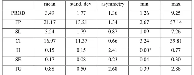
Table 1 shows the basic statistics for the seven variables; most roughly follow the pattern of our key variable, PROD, with a positive asymmetry indicating that the maximum can be much larger than the mean, though all coefficients of variation are lower than 0.68 (with the exception of H). A slight negative asymmetry is present only for SE. Some extreme values can be quite wild, as in the case of H and TG. The maximum technological gap of 2.88 shows that domestic firms can be more productive than the foreign ones; what is indeed true for sectors 37 and 39. The former is basic metallurgy (see the Appendix) which is predominantly Portuguese, while the latter is a more heterogenous bunch of firms where it is difficult to identify a definite foreign skill. The above information is complemented by Table 2, giving the year averages, by sector, for each variable. Sectoral variations are quite large, for all variables4.
Table 1
Descriptive statistics of the seven variables
mean stand. dev. asymmetry min max
PROD 3.49 1.77 1.36 1.26 9.25
FP 21.17 13.21 1.34 2.67 57.14
SL 3.24 1.79 0.87 1.09 7.26
CI 16.97 11.37 0.66 3.24 39.81
H 0.15 0.15 2.41 0.00* 0.77
SE 0.17 0.08 -0.23 0.04 0.30
TG 0.88 0.50 2.68 0.39 2.88
* In sector 39 there is great dispersion and the Herfindahl was approximated to zero.
4
Figures 1 and 2 show the dispersion diagrams of PROD with FP and TG, respectively. There is no clear positive trend of the domestic productivity either with FP or TG.
Table 2
Sector averages
31 32 33 34 35 36 37 38 39
PROD 5.1 1.6 2.5 4.7 6.9 3.3 2.9 2.4 2.1
FP 23.8 19.1 8.0 16.5 20.3 22.1 6.4 52.5 21.8
SL 1.7 7.1 3.6 1.3 1.2 4.3 2.9 2.9 4.2
CI 15.1 5.4 10.0 32.3 34.2 18.0 24.6 9.6 3.5
H 0.10 0.09 0.03 0.17 0.11 0.11 0.48 0.24 0.00 SE 0.19 0.26 0.28 0.16 0.05 0.19 0.19 0.17 0.07 TG 0.83 0.87 0.76 0.56 0.69 0.54 2.04 0.56 1.08
0,0 2,0 4,0 6,0 8,0 10,0
0,0 10,0 20,0 30,0 40,0 50,0 60,0
FP
PROD
Figure 1
Dispersion diagram: FP (horizontal axis) x PROD (vertical axis)
Figure 2
0,0 2,0 4,0 6,0 8,0 10,0
0 50 100 150 200 250 300 350
TG
PROD
2.2. THE STANDARD SPECIFICATION
We start with Kokko´s (1992) specification, assuming labour productivity of the locally-owned firms to be a function of the foreign affiliates´market share and various other industry characteristics. Our dependent variable is thus the productivity of domestic firms (PROD) and, to account for the spillovers effect, we use the variable foreign presence (FP), previously defined.
With the proviso that labour productivity is at best a partial measure of overall multi-factor productivity5, if spillovers occur, there should be higher productivity levels for domestically-owned firms in sectors with a larger foreign presence. Variable FP should have a significant positive coefficient.
As the amount of technology that could potentially spill over to local firms is probably not exogenously given, but dependent on both host country and industry characteristics, we chose as control variables the skill of the labour force (SL), the capitalistic intensity (CI), the degree of competition (H) and the level of economies of scale of domestic firms (SE). The first three variables are computed using all firms in the sector. It could appear more appropriate to build these variables, especially SL and CI, using domestic firms only, as our purpose is to control for influences on domestic productivity; but data limitations did not afford it. In any case, the overall sectoral figures inform about the “environment” domestic firms face and seem acceptable if the results´ interpretation is properly done.
5
We expect a positive relation between SL, SE, CI and domestic productivity. On what concerns the Herfindhal index, it measures the degree of (producers´) concentration in each industry and is included to account for the effect of market power on the value of productivity. It is generally agreed that more concentrated industries are better able to engage in monopoly pricing and should therefore display higher labour productivity. However, if the larger firms are foreign, which is mostly the case in Portugal, this relation may not occur. Besides, a high concentration level may imply that, due to limited competition, there are not conditions favourable to the spillovers diffusion. In extreme cases, it is even possible that the foreign (sub-)sector performs as an enclave, producing a dual structure at the sectoral level. The expected sign for H is then not pre-defined.
The following equation was our starting point:
PRODit = α+ β1FPit +β2CIit +β3SEit +β4Hit +β5SLit+∈it (1)
where ∈it refers to the disturbance term for the ith unit (sector) at time (year) t.
If we assume that the disturbances are uncorrelated through time and units, and -conditioned on the explanatory variables - identically distributed with a zero mean, this is a pooled regression model which can be consistently and efficiently estimated by ordinary least squares. Table 3, column (1), displays the results of this estimation. The only positive determinants on domestic productivity are the capitalistic intensity and the skilled labour variables. The concentration index is significant but with a negative sign. The foreign presence is not significant and thus the expected spillover effect is not confirmed.
3. THE INFLUENCE OF THE TECHNOLOGICAL GAP
3.1. THE GAP AND FOREIGN PRESENCE
technological level of multinationals´ affiliates compared to that of domestic firms. Two opposing arguments can be found concerning the effect of this gap on actual technology transfer. If the technological capabilities gap between the two sets of firms is too large,
Table 3
Spillovers and technological Gap
Indep. Variables (1) (2) (3)
C 1.19 (2.57) .06 (.06) .30 (.46) FP 0.86 (1.44) 2.41 (1.68) CI .089 (3.17) .11 (3.11) .12 (3.23) SE -.82 (0.48) .45 (.24) .93 (.53) H -3.43 (3.20) -5.13 (2.58) -4.24 (2.97) SL 2.95 (2.54) 2.75 (2.28) 2.47 (2.01) TG .66 (1.25) FPXTG 4.08 (1.96)
R² .814 .828 .827
Adj R² .783 .792 .798
F 26.33 23.23 28.16
t-values (between brackets) using White´s heteroscedasticity correction
domestic firms may not be able to benefit from the introduction of new technology; in fact, the affiliates´ technology may be too advanced to allow for any interaction with local firms, so that higher technology gaps only serve to insulate the affiliates from the local firms. On the other hand, if the technology gap is too small, foreign investment may transmit few benefits to domestic firms. A certain distance (in technology) appears then necessary for spillovers to occur as, for instance, when local firms copy foreign procedures or benefit from the training of local employees.
We refine our analysis by including variable TG, for the technological gap, in model (1). By assuming that a higher productivity signals a better technology, TG is indeed an indirect measure of the gap; moreover, notice that – for values below 1 – the higher the gap the lower is TG.
The new model is:
where ∈it has the same properties as in (1).
Table 1, column (2), displays the estimation results. The proxy for spillovers diffusion, FP, now becomes significant (at the 10% level) and its coefficient also increases. This leads us to suspect, in the line of Kokko (1992) 6, that the technological gap is indispensable for the spread of FDI indirect effects. However, the very coefficient of the proxy for the technological gap, though positive, is not significant.
Remembering that, even if FP is high, a high gap (i.e. a low TG) would not be favourable to spillovers, we built a new variable to portray the interaction between FP and TG: FPxTG. Several modelling options are then available using this interaction term, depending on whether FP and TG themselves are included in the equation. The results do not differ much, and those for the most parsimonious model:
PRODit= α+ β1FPxTGit +β2CIit +β3SEit +β4Hit +β5SLit +∈it (3)
are displayed in column (3) of Table 3 and confirm the crossed effect.
3.2. THE GAP RANGE
If the technological gap matters, the fact that it is not significant in model (2) can also be associated to its different levels across sectors. The question we then seek to answer is how large should the gap be in order to (i) have a positive effect; (ii) maximize the spillovers diffusion. Consequently, a test of the sensitivity of the model to alternative ranges for the technological gap was performed.
We investigated several alternatives by “cutting” variable TG outside the set ranges. If we define a dummy with value one whenever the TG values are within the pre-defined range and zero otherwise, the “cut variable” is equal to the dummy times TG. The dummy itself has also been included in the model, to allow for extra flexibility:
PRODit= α+ β1FPit +β2CIit +β3SEit +β4Hit +β5SLit +β6Dit +β7TGxDit +∈it . (4)
Table 4 shows the results for the alternative ranges tried. The gap variables within a lower bound of 40% are not significant, signalling that the gap cannot be too
6
high. The best results occur for the 50-80% range, where the product variable displays the highest t-values and also the highest coefficients are found.
We keep this range for further specifications of the model.
Table 4
Testing alternative ranges for the technological gap.
Indep. Variables Gap 40-50% Gap 40-95% Gap 50-80% Gap 50-95% Gap 60-95%
C .89 (1.70) 1.04 (2.24) .80 (1.30) .69 (1.29) .86 (1.91) FP 2.57 (1.58) 1.33 (1.74) 2.99 (2.39) 2.37 (2.38) 1.39 (1.71) CI .11 (2.70) .10 (3.05) .09 (3.85) .10 (3.14) .10 (3.57) SE -.88 (.47) -.93 (.43) -1.37 (.75) -1.07 (.45) -1.95 (.87) H -3.70 (2.58) -3.63 (3.26) -2.56 (2.98) -2.95 (2.40) -3.06 (3.22) SL 2.29 (1.50) 2.75 (1.94) 3.16 (2.71) 3.24 (2.39) 2.93 (2.41) D40/80 -3.45 (1.81) D40/80.TG 4.97 (1.80) D40/95 -.29 (.56) D40/95.TG .45 (.69) D50/80 -6.18 (3.42) D50/80.TG 8.85 (3.46) D50/95 -3.11 (2.78) D50/95.TG 4.15 (2.71) D60/95 -3.58 (2.06) D60/95.TG 5.01 (2.23)
R² .853 .823 .894 .858 .852
Adj. R² .816 .778 .868 .823 .815
F 23.12 18.57 33.86 24.26 23.04
t-values (between brackets) using White´s heteroscedasticity correction.
exercise confirms is the key role of the gap range for ensuring the occurrence of spillovers.7
4.A MODEL WITH VARIABLE SPILLOVER COEFFICIENTS
In the previous specifications the vector of parameters β is assumed constant through all sectors and years. In the case of the variable FP this does not seem to be reasonable because its values are quite differentiated along the sectors. Basic statistics (see Table 2) show a sector with a highly significant weight of foreign affiliates (sector 38, which includes machinery and transport equipment), two with a low weight (sectors 33, wood and cork, and 37, basic metallurgy), and the remaining ones with values for foreign presence around the global average.
We then estimated the influence of foreign presence disaggregating FP in model (4) according to this grouping:
PRODit= α +β1FP1it +β2FP2it +β3FP3it +β4CIit +β5SEit +β6Hit +β7SLit +β8D50/80it
+β9D50/80xGTit +∈it , (5)
where FP1 includes only sector 38, FP2 sectors 33 and 37 and FP3 the remaining ones (31, 32, 34, 35, 36 and 39); FP = FP1+ FP2+ FP3.
Results are shown in Table 5, column (1). We also tried out a different grouping, including sector 38 in the largest previous group (column (2)). In the first case only sector 38 presents positive, significant spillovers, an expected result due to the high share of foreign presence in it (52.5 on average). The influence of sector 38 is confirmed in the second grouping.
5. A FIXED EFFECTS MODEL
It is possible that a myriad of influences on productivity – like those related to the “software” environment for spillovers mentioned by Kokko, as well as to other sectoral specifics - are not included in the right-hand-side of our equations. These
7
missing or unobserved variables can be assumed to express the heterogeneity of the individual units, but to be constant over time. A common formulation of such a model states that differences across units can be captured in differences in the constant term. It can be written as:
PRODit= β1FPit +β2CIit +β3SEit +β4Hit +β5SLit +β6Dit +β7TGxDit +∈it (6)
where ∈it = αi + ηit , with the ηit zero-mean, constant variance shocks uncorrelated
across time and units and the αi being the unknown individual effects to be estimated for
each unit (sector) i.
Table 5
Panel Data: Different groups of sectors for FP
Indep. variables (1) (2)
C 1.37 (1.53) .79 (1.16) CI .010 (3.92) .09 (3.84) SE -1.75 (.84) -1.40 (.74) H -3.42 (2.93) -2.58 (3.07) SL 3.05 (2.46) 3.17 (2.62) D50/80 -7.10 (2.99) -6.18 (3.29) D50/80TG 9.99 (3.07) 8.85 (3.78) FP38 3.08 (1.83) FP33/37 -1.01 (.16) 3.44 (.61) FP31/32/34/35/ 36/39 .52 (.21) FP31/32/34/35/ 36/38/39 3.03 (1.89)
R² .899 .894
Adj. R² .865 .863
F 25.86 28.55
t-values (between brackets) using White´s heteroscedasticity correction .
The individual effects may be either fixed or random. In the latter case, though the αi must be uncorrelated with the explanatory variables, the errors in (6) will be
effects estimator will still produce consistent estimates of the identifiable parameters8. If the number of units is small enough, model (6), under the fixed effects assumption, can be estimated by ordinary least squares with one column for each sectoral dummy. The result of this estimation is reported in Table 6.
It is interesting to compare the coefficients in Table 6 with those in the related column of Table 4. The four significant independent variables in the fixed-effects model are as well in Table 4, with the same signs and also, but for the concentration index (H),
Table 6
Fixed effects model – least squares estimation Independent Variables Coefficients
FP -5.16
(1.71)
CI .17
(3.56)***
SE -4.36
(1.06)
H -8.84
(3.88)***
SL -3.2 5
(.92)
D31 6.99
(3.95)***
D32 3.95
(3.26)***
D33 3.50
(2.78)**
D34 5.32
(2.49)**
D35 6.13
(2.94)***
D36 4.11
(3.37)***
D37 5.25
(3.28)***
D38 8.52
(3.90)***
D39 3.73
(4.15)***
D50/80 -5.14
(2.79)** D50/80TG 7.27
(2.89)***
R² .957
Adj R² .924
F 29.52
t statistics with White’s heteroscedasticity correction
8
roughly the same value. Two major changes then occur for variables FP and SL: their coefficients change sign and become not significant. On the other hand, all idiosyncratic effects are positive and significant – most at the 1% level – showing that there clearly exists a sectoral effect. Indeed, it seems to be more important than those previously accounted for the foreign presence (FP) and the skilled labour ratio (SL).
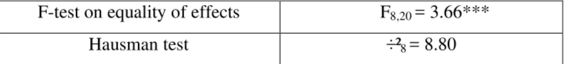
Table 7 presents the results of two tests. The first is a standard F test to check the null hypothesis that the sectoral effects are all equal. Under this null, the efficient estimator is a pooled least squares, and the ratio:
Fn-1, nT-n-k = [ (R2u-R2r) / (1-R2u) ] x [(nT-n-k) / (n-1)]
where u indicates the unrestricted model, r the restricted one, n stands for the number of units, T for that of periods and k for the number of explanatory variables, is asymptotically an F. In our case, the corresponding lines in Tables 4 and 6 provide the R² values for computing the F8,20 statistic. The null is clearly rejected at 1%.
The second is the Hausman test statistic, which tests the null hypothesis that the (random) effects are uncorrelated with the explanatory variables. Though the null is not rejected9, the fact that the random effects model “passes” the test may indicate that, for instance, there is not enough variation in the explanatory variables to provide results precise enough to distinguish between the two sets of estimates (see Johnston and Dinardo (1997), p. 404).
Table 7
Two tests on the fixed effects model F-test on equality of effects F8,20 = 3.66***
Hausman test ÷²8 = 8.80
The results in this section show that there are significant sector specific effects to be considered when explaining the productivity variation; the adjusted R2 increases from 0.868 in Table 4 to 0.924 in Table 6. According to the fixed–effects estimates, the inclusion of sectoral specifics, on purging the other estimators of this effect, apparently changes the empirical role of foreign presence on the determination of domestic productivity.
9
6. IN SEARCH OF INTER-SECTORAL SPILLOVERS
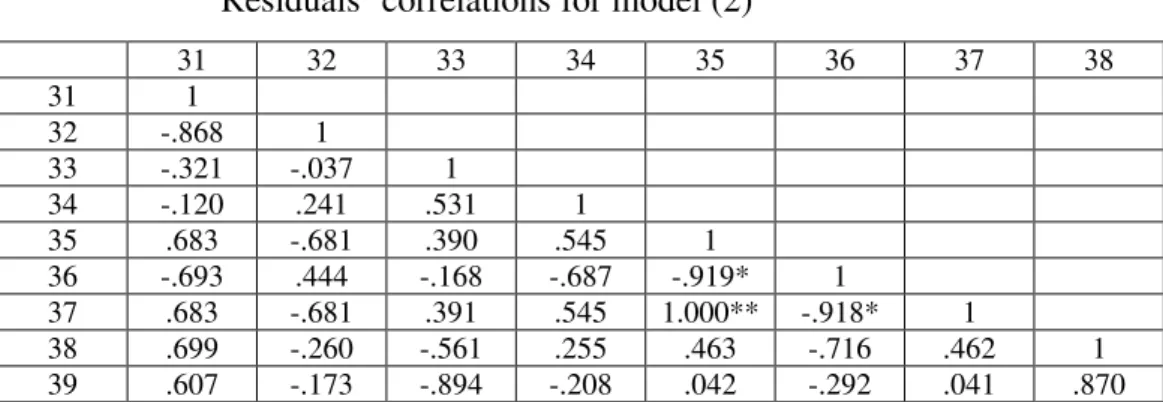
Table 8 shows the correlation coefficients for the residuals in model (2), computed on a sectoral basis. Given that the residuals account for productivity shocks unexplained by the model, a high positive correlation would signal a common (hidden) effect on the two sectors productivity. By the same token, high negative correlations would mean opposing factors in the sectors performance.
If we consider only correlations higher than 0.5 in absolute value, three sectors oppose the other six. Indeed, high negative correlations are associated with textiles (32), wood and cork (33) and non-metallic (36), which, however, have no correlation link between themselves. These three groups stand for traditional groups of manufactures with a strong historical presence in the Portuguese economy. Among those positively correlated, two pairs show a close association: chemicals and metallurgy (35 and 37) and transport and others (38 and 39), signalling that the pairs are indistinguishable, in terms of the productivity residual. Given the diversity of goods encompassed by each of these four sectors, this may be partially due to the unfortunately high aggregation level of our study, but also suggests an identity of reaction to other factors. We venture that such factors might be a combination of centrifugal and centripetal effects, in the lines of Fujita et al. (1999), responsible for agglomerations like the one in the Greater Lisbon industrial area, where many of those firms are located. It is telling, however, that no direct strong correlation exists between the two pairs. Of the remaining two sectors, food (31) is worth mentioning, due to its relevant correlation linkages to six of the other eight sectors.
Table 8
Residuals´ correlations for model (2)
31 32 33 34 35 36 37 38
31 1
32 -.868 1
33 -.321 -.037 1
34 -.120 .241 .531 1
35 .683 -.681 .390 .545 1
36 -.693 .444 -.168 -.687 -.919* 1
37 .683 -.681 .391 .545 1.000** -.918* 1
Overall, on exploratory grounds - given the reduced number of years in our panel -, the residuals analysis points to a broad separation between less advanced, more traditional industries and more modern ones, suggesting that maybe a sharper characterisation of the technological level of each sector is missing. Nevertheless, the aggregation level of the study puts a grain of doubt on the utility and the feasibility of constructing this new explanatory (and likely omitted) variable.
7. CONCLUSIONS
Any result on the existence of spillovers as indicated by the foreign presence effect on the productivity level of domestic enterprises must be cautiously taken. As pointed out before, the concept of technological spillovers is quite vast and abstract. Notwithstanding, the analyses in the previous sections have produced a few new insights.
Firstly, we confirmed that the relationship between foreign presence and productivity is a complex one, being only revealed if the proper controls on these two variables are used. It is possible that, in some cases, we do not identify spillovers not because they do not exist but simply because they are not increasing linearly with the foreign presence. This nonlinearity is suggested by the fact that a technological gap seems to be a condition for spillovers, but only within a certain range. We clearly showed this, first by detecting a significant interaction between these two variables and then by progressively arriving at “an optimal gap range” for spillovers.
We also showed that a crucial influence, of a sectoral nature, is present. Indeed, for many sectors, even within the “optimal range” spillovers do not take place. They seem to favour modern sectors, with large scale gains, not existing before in the economy. However, the results of the fixed-effects model indicate that other variables are needed to account for these differences, as also suggested by the residuals analysis.
Finally, productivity shocks not described by the variables studied show common patterns among the sectors. Further econometric work using this information should be pursued, using techniques like Zellner´s seemingly unrelated regressions, provided that more years are made available.
issues. There is also interest in identifying technology spillovers at a more detailed level, using as the dependent variable measures of improvement as R&D expenditures, labour skills, cost of inputs or the managers´ turnover. Last but not least, work with disaggregated data at the firm level would be relevant to confirm these findings, as firms can be highly heterogeneous in a given sector.
APPENDIX
General description of the nine manufacturing sectors (between brackets appears the name they are usually referred to in the text, if different from the description)
31: Food and tobacco
32: Textiles, clothing and leather goods 33: Wood and cork
34: Paper, printing and publishing
35: Chemicals, rubber and plastics (chemicals) 36: Minerals, non metallic
37: Basic metallurgy
38: Steel goods, machines and transport material 39: Other manufactures
References
Aitken, B. and A. Harrison (1997), “Do Domestic Firms Benefit form Foreign Direct Investment”, Columbia University, Mimeo.
Blomström, M. (1986), «Foreign Investment and Productive Efficiency: the Case of Mexico»,
The Journal of Industrial Economics, vol. XXXV, nº 1, pp. 97-110
Blomström, M. and H. Persson (1983), «Foreign Investment and Spillover Efficiency in an Underdeveloped Economy: Evidence from the Mexican Manufacturing Industry»,
World Development, vol. 11, pp. 493-501
Blomström, M. and E. Wolff (1994), «Multinational Corporations and Productivity Convergence in Mexico», in Convergence of Productivity, Cross National Studies and Historical Evidence, ed. by W. Baumol, R. Nelson and E. Wolff, Oxford University Press, Oxford, pp. 263-284.
Djankov, S. and Hoekman, B. (1999), «Foreign Investment and Productivity Growth in Czech Enterprises», forthcoming in World Bank Economic Review.
Farinha, F. and J. Mata (1996), “The Impact of Foreign Direct Investment in the Portuguese Economy”, W/P nº 16/96, Bank of Portugal.
Fujita, M. Krugman, P and A. Venables (1999), The Spatial Economy-Cities, Regions and International Trade, The MIT Press, Cambridge
Harrison, A. (1996), «Determinants and Consequences of Foreign Investment in Three Developing Countries», in Mark Roberts and James Tybout (eds), Industrial Evolution in Developing Countries: Micro Patterns of Turnover, Productivity and Market Structure, Oxford, Oxford University Press
Johnston, J. and J. Dinardo (1997) Econometric Methods, 4th ed., McGraw-Hill.
Judge, G. G., W. E. Griffiths, R. Carter Hill, H. Lütkepohl and T.-C. Lee. (1985), The Theory and Practice of Econometrics, 2nd ed. New York, John Wiley & Sons.
Kokko, A. (1992), Foreign Direct Investment, Host Country Characteristics, and Spillovers, Ph. D. Thesis, Stockholm School of Economics
Mateus, A. M. 1998. Economia Portuguesa. Lisbon, Editorial Verbo.