❊s❝♦❧❛ ❞❡
Pós✲●r❛❞✉❛çã♦
❡♠ ❊❝♦♥♦♠✐❛
❞❛ ❋✉♥❞❛çã♦
●❡t✉❧✐♦ ❱❛r❣❛s
◆◦ ✹✺✺ ■❙❙◆ ✵✶✵✹✲✽✾✶✵
❋♦r❡✐❣♥ ❉✐r❡❝t ■♥✈❡st♠❡♥t ❙♣✐❧❧♦✈❡rs✿ ❆❞❞✐✲
t✐♦♥❛❧ ▲❡ss♦♥s ❋r♦♠ ❛ ❈♦✉♥tr② ❙t✉❞②
❘❡♥❛t♦ ●❛❧✈ã♦ ❋❧ôr❡s ❏✉♥✐♦r✱ ▼❛r✐❛ P❛✉❧❛ ❋♦♥t♦✉r❛✱ ❘♦❣ér✐♦ ●✉❡rr❛ ❙❛♥t♦s
❙❡t❡♠❜r♦ ❞❡ ✷✵✵✷
❋✉♥❞❛çã♦ ●❡t✉❧✐♦ ❱❛r❣❛s✳
❊❙❈❖▲❆ ❉❊ PÓ❙✲●❘❆❉❯❆➬➹❖ ❊▼ ❊❈❖◆❖▼■❆ ❉✐r❡t♦r ●❡r❛❧✿ ❘❡♥❛t♦ ❋r❛❣❡❧❧✐ ❈❛r❞♦s♦
❉✐r❡t♦r ❞❡ ❊♥s✐♥♦✿ ▲✉✐s ❍❡♥r✐q✉❡ ❇❡rt♦❧✐♥♦ ❇r❛✐❞♦ ❉✐r❡t♦r ❞❡ P❡sq✉✐s❛✿ ❏♦ã♦ ❱✐❝t♦r ■ss❧❡r
❉✐r❡t♦r ❞❡ P✉❜❧✐❝❛çõ❡s ❈✐❡♥tí✜❝❛s✿ ❘✐❝❛r❞♦ ❞❡ ❖❧✐✈❡✐r❛ ❈❛✈❛❧❝❛♥t✐
●❛❧✈ã♦ ❋❧ôr❡s ❏✉♥✐♦r✱ ❘❡♥❛t♦
❋♦r❡✐❣♥ ❉✐r❡❝t ■♥✈❡st♠❡♥t ❙♣✐❧❧♦✈❡rs✿ ❆❞❞✐t✐♦♥❛❧ ▲❡ss♦♥s ❋r♦♠ ❛ ❈♦✉♥tr② ❙t✉❞②✴ ❘❡♥❛t♦ ●❛❧✈ã♦ ❋❧ôr❡s ❏✉♥✐♦r✱ ▼❛r✐❛ P❛✉❧❛ ❋♦♥t♦✉r❛✱ ❘♦❣ér✐♦ ●✉❡rr❛ ❙❛♥t♦s ✕ ❘✐♦ ❞❡ ❏❛♥❡✐r♦ ✿ ❋●❱✱❊P●❊✱ ✷✵✶✵
✭❊♥s❛✐♦s ❊❝♦♥ô♠✐❝♦s❀ ✹✺✺✮
■♥❝❧✉✐ ❜✐❜❧✐♦❣r❛❢✐❛✳
FOREIGN DIRECT INVESTMENT SPILLOVERS: ADDITIONAL
LESSONS FROM A COUNTRY STUDY *
Renato G. Flôres Jr.a
EPGE / Fundação Getúlio Vargas Praia de Botafogo 190, 11° andar Rio de Janeiro 22253-900 Brazil
Maria Paula Fontoura
ISEG / Universidade Técnica de Lisboa Rua Miguel Lupi 20
Lisbon 1249-078 Portugal
Rogério Guerra Santos
ISEG / Universidade Técnica de Lisboa Rua Miguel Lupi 20
Lisbon 1249-078 Portugal
a
Corresponding author:
phone (55 21) 2559 5909; fax (55 21) 2553 8822; e-mail [email protected].
(August, 28; 2002)
FOREIGN DIRECT INVESTMENT SPILLOVERS: ADDITIONAL
LESSONS FROM A COUNTRY STUDY
Abstract
We investigate the impact of foreign direct investment on the productivity of domestic firms, using sectoral data for Portugal. An improved analysis takes into account the most appropriate interval for the technological gap between foreign and domestic firms. Sectoral variation of spillovers, idiosyncratic sectoral factors and the search for inter-sectoral effects provide new insights on the subject. Significant spillovers require a proper technology differential between the foreign and domestic producersandfavourable sectoral characteristics. Broadly, they occur in modern industries in which foreign firms have a clear, but not too sharp, edge on the domestic ones. Agglomeration effects are also identified as pertinent specific influences.
Keywords: agglomeration effect; domestic productivity; foreign direct investment; Portugal; spillovers; technology gap.
1. INTRODUCTION
Historically, foreign direct investment (FDI) meant capital inflows and
additional employment. In a world of financial crises, volatile credibility and footloose
industrial plants, what does FDI mean? One major benefit, much cited in the literature
of the past decade, is the increase in domestic firms’ productivity. This is related to the
concept of technology or productivity spillovers, which embodies the fact that foreign
enterprises own intangible assets - such as technological know-how, marketing and
managerial skills, international experience or reputation - which can be transmitted to
domestic firms, raising their productivity level.
Spillovers are a matter of externalities within the country, from established
foreign producers to domestic ones, and may be linked to two groups of effects:
knowledge spillovers and competitive disciplinary effects. Main examples of the former
are: (i) new technology, either embodied in imported inputs and capital goods or sold
directly through licence agreements, or transferred to domestic producers who learn new
techniques from their foreign buyers; (ii) learning by doing among domestic firms,
combined with investments in formal education and on-the-job training of domestic
employees who move from foreign to domestic firms; (iii) cost savings due to
technology passed to downstream users of new products or upstream buyers or
suppliers. Competitive effects, or rather, incentives to competition resulting from the
foreign affiliates entrance, operate through either a more efficient use of existing
technology and resources or a search for more efficient technologies, or a restraint on
the exercise of market power by domestic firms.
The spillover concept has thus a meaning broader than imitation or even
“knowledge effect” is inherently an abstract concept, comprising not only knowledge
and skills transfer but also “the means for using and controlling factors of production”
(Kokko (1992), p. 21), such as product, process and distribution technology or
management skills. No wonder, with a lack of more formal theoretical modelling,
empirical evidence on spillovers diffusion is ambiguous, as surveys like Blomström and
Kokko (1998) or Görg and Strobel (2001) show. Though recent studies point more
favourably to a significant relationship, this is usually accompanied by important
qualifications.
Blomström (1986), using sectoral data, found that an increase in foreign
presence failed to increase the productivity growth of Mexican firms. Santos (1991) also
did not find a positive influence on the productivity level for the case of Portugal, in the
period 1977-82. Conversely, Blomström and Persson (1983) and Blomström and Wolff
(1994) found that domestic labour productivity is positively influenced by foreign
presence.
Micro-econometric studies with panel data on enterprises (or establishments) are
in general more supportive of a negative influence. Notwithstanding, Farinha and Mata
(1996) found a positive effect of FDI on the productivity of domestic firms in Portugal,
with data at the firm level, covering the 1986-92 time period. Haddad and Harrison
(1993), Harrison (1996) and Aitken and Harrison (1997) found a negative significant
relationship between the size of foreign presence and the productivity of domestic firms,
while Sjöholm (1997) raised relevant qualifications. Later, Aitken and Harrison (1999)
better qualified their results, by raising the idea of a compromise between a positive
effect on foreign owned firms and a negative one, on those domestically owned. A
joint ventures and FDI, as regards Czech firms without such links, is also found in
Djankov and Hoekman (2000).
The case study literature, on the other hand, seems to point more clearly to
positive spillovers, as in Rhee and Belot (1989), in spite of the existence of mixed
evidences, as Mansfield and Romeo (1980)´s classical enquiry.
All this raises the suspicion that the empirical studies can be suffering from a
specification problem. Indeed, at present, the theory does not provide testable, dynamic
structural models of spillovers’ impact on the productivity of domestic enterprises. The
negative results might thus be related to missing explanatory variables, to a poor
characterization of the channels through which spillovers take place, including the
absence of temporal effects, and to confusion, in the reduced forms used, between
product and input markets determinants.
In this paper we concentrate on the impact of foreign investment on the
productivity performance of Portuguese firms. The study is conducted for the
manufacturing sector at the two-digit level. Data restrictions limited us to nine groups
(or sectors), for the period 1992-95. Notwithstanding, the panel nature of the data
allows to bypass somehow the relatively small sample size, going beyond a pooled
analysis and using techniques particularly appropriate to exploit the sector specificities.
When Portugal joined the European Union (EU) in 1986, foreign direct
investment as a percentage of GDP had never passed the 1% threshold. After 1988, this
ratio reached a peak of 4% in 1990 and, though it has continuously decreased since
then, it has never crossed back the 1% line1. This, apart from the points mentioned
below, obviously raises interest on the indirect effects of FDI in the country, as a
subject. Not only should the Portuguese results be contrasted with findings for selected
developing economies, but they should as well be compared with those from other
“emerging” EU economies, like Ireland and Greece.
Though still resorting to static, single equation modeling, we innovate with
respect to previous studies by not only including variables which control for other
productivity shocks but, especially, by searching the most appropriate interval on what
concerns the influence of the “technological gap” on spillovers diffusion. This has
important development policy implications, as the results suggest that outside a given
range of distances between the domestic and foreign technological levels spillovers do
not take place.
Sectoral variation in the spillovers effect, and the identification of specific
sectoral factors are also tested. Evidence is provided on a strong relationship between
the spillovers process and the idiosyncratic sector characteristics.
Finally, we tried to identify, in an exploratory way, inter-sectoral positive
spillover effects. This led us to uncover the possibility that geographic factors, notably
agglomeration effects, may play an important role in spillovers diffusion; and should
consequently be included in future research.
In what follows, section 2 presents the data set and the basic model. Section 3
investigates the best range for the technological gap, while in section 4 a varying
spillover coefficient, according to the industry groups, is used. This approach is
continued in the next section, where a fixed-effects model is studied. Section 6 exploits
the panel structure of the residuals to draw an exploratory picture of inter-sectoral
leads to consider the role of agglomeration effects. Favorable evidence is provided on
them. A final section concludes.
Though reaffirming that the relationship between domestic firms productivity
and foreign presence is a complex one, we claim that it does take place in a positive
way, if a proper technology differential between the foreign and domestic producers
existsand the sectoral characteristics are favorable. We clearly showed the interaction
of these two factors with the spillover effect, but a better grasp of the sectoral conditions
is needed. Those associated to modern, more globalized industries, in which the foreign
owned establishments have a clear though not too sharp edge on the domestic ones
seem to enhance the spillovers. Intersectoral effects may significantly count, and other
specific influences, notably agglomerative location factors, can also be pertinent. For
developing economies, this highlights the need to combine FDI policies with the
regional development pattern.
2. THE BASIC MODEL
(a)Preliminary analyses
Our sample comprises 36 observations related to nine manufacturing sectors, for
the period from 1992 to 1995. The data come from the Inquérito às Empresas
Harmonizado conducted annually by the Instituto Nacional de Estatística – INE2. This
survey investigates all manufacturing firms with 100 or more employees, which are
believed to represent at least 80 per cent of total employment and of value added by
manufactures.
The sectors correspond to the two-digit level of the standard industrial
Seven variables were computed at the yearsxsectors level:
PROD (productivity of the domestic firms; in million escudos per worker) – total value
added divided by the number of workers;
FP (foreign presence) - the ratio of value added by all foreign firms to total value added;
SL (skilled labor) - the ratio of white collar to blue collar employees;
CI (capitalistic intensity, in million escudos per worker) - total fixed assets divided by
the number of workers;
H (a concentration index) - the ratio of the total number of employees in firms with 500
or more employees to total employment in the sector;
SE (scale economies) – the ratio of the average output of domestic enterprises to the
average output of firms with 500 or more employees;
DP (domestic performance) – defined as the ratio of domestic firms’ productivity to the
productivity of foreign enterprises.
Variable DP is a key element in our analysis. It is related to the technological
gap between the domestic and foreign producers; the lower its values the higher the gap.
An alternative specification would be to define a variable equal to 1-DP, which would
directly portray the gap.
Table 1 shows the basic statistics for the seven variables; most roughly follow
the pattern of our key variable, PROD, with a positive asymmetry indicating that the
maximum can be much larger than the mean, though all coefficients of variation are
lower than 0.68 (with the exception of H). A slight negative asymmetry is present only
for SE. Some extreme values can be quite wild, as in the case of H and DP. The
maximum performance of 2.88 shows that domestic firms can be more productive than
sectors definitions). The former is basic metallurgy, which is predominantly Portuguese,
while the latter – other manufactures - is a rather heterogeneous bunch of firms where it
is difficult to identify a definite foreign skill.
Table 2, giving the year averages, by sector, for each variable, complements the
above information. Sectoral variations are quite large, for all variables3.
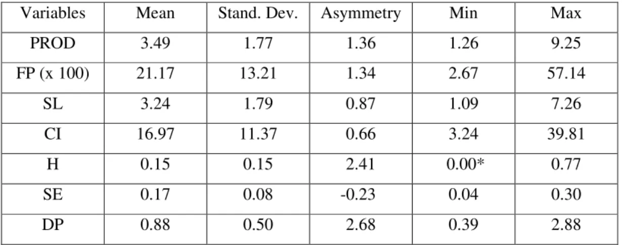
Table 1.Descriptive statistics of the seven variables
Variables Mean Stand. Dev. Asymmetry Min Max PROD 3.49 1.77 1.36 1.26 9.25 FP (x 100) 21.17 13.21 1.34 2.67 57.14
SL 3.24 1.79 0.87 1.09 7.26
CI 16.97 11.37 0.66 3.24 39.81
H 0.15 0.15 2.41 0.00* 0.77
SE 0.17 0.08 -0.23 0.04 0.30
DP 0.88 0.50 2.68 0.39 2.88
*In sector 39 there were no firms with 500 or more employees.
Table 2.Sector averages
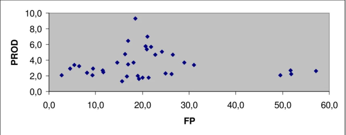
Figures 1 and 2 show the dispersion diagrams of PROD with FP and DP,
respectively. There is no clear positive trend of the domestic productivity either with FP
or DP. Actually, in both graphs, there is a strong suggestion of nonlinear effects and a
hint of possible outliers.
Figure 1.Dispersion diagram: FP (horizontal axis) x PROD (vertical axis)
Figure 2.Dispersion diagram: DPx100 (horizontal axis) x PROD (vertical axis)
0,0 2,0 4,0 6,0 8,0 10,0
0,0 10,0 20,0 30,0 40,0 50,0 60,0
FP
P
R
O
D
0,0 2,0 4,0 6,0 8,0 10,0
0 50 100 150 200 250 300 350
DP
P
R
O
(b)The standard specification
We started with Kokko´s (1992) specification, assuming labor productivity of
the locally owned firms to be a function of the foreign affiliates’ market share and
various other industry characteristics. Our dependent variable is thus the productivity of
domestic firms (PROD) and, to account for the spillovers effect, we follow the common
practice to use the variable foreign presence (FP), previously defined.
With the proviso that labor productivity is at best a partial measure of overall
multi-factor productivity4, if spillovers occur, there should be higher productivity levels
for domestically owned firms in sectors with a larger foreign presence. Variable FP
should then have a significant positive coefficient.
As the amount of technology that could potentially spill over to local firms is
probably not exogenously given, but dependent on both host country and industry
characteristics, we chose as control variables the skill of the labor force (SL), the
capitalistic intensity (CI), and proxies for the degree of competition (H) and the level of
economies of scale of domestic firms (SE). The first three variables are computed using
all firms in the sector. It could appear more appropriate to build these variables,
especially SL and CI, using domestic firms only, as our purpose is to control for
influences on domestic productivity; but data limitations did not afford it. In any case,
the overall sectoral figures inform about the “environment” domestic firms face and
seem acceptable if the results´ interpretation is properly done.
We expect a positive relation between SL, SE, CI and domestic productivity. On
what concerns variable H, it measures the degree of (producers’) concentration in each
industry and is included to account for the effect of market power on the value of
engage in monopoly pricing and should therefore display higher labor productivity.
However, if the larger firms are foreign, which is mostly the case in Portugal, this
relation may not occur. Besides, a high concentration level may imply that, due to
limited competition, there are not conditions favorable to the spillovers diffusion. In
extreme cases, it is even possible that the foreign (sub-)sector performs as an enclave,
producing a dual structure at the sect oral level. The expected sign for H is then not
pre-defined.
The following equation was our starting point:
PRODit=α+β1FPit+β2CIit+β3SEit+β4Hit+β5SLit+∈it , (1)
where∈itrefers to the disturbance term for the i-th unit (sector) at time (year) t.
If we assume that the disturbances are uncorrelated through time and units, and
-conditioned on the explanatory variables - identically distributed with a zero mean, this
is a pooled regression model which can be consistently and efficiently estimated by
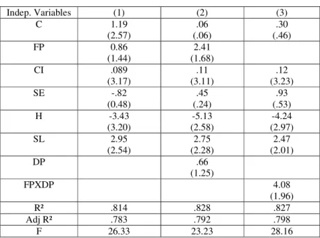
ordinary least squares. Column (1), in Table 3, displays the results of this estimation.
The only positive determinants on domestic productivity are the capitalistic intensity
and the skilled labor variables. The concentration index is significant but with a
negative sign. The foreign presence is not significant and thus the expected spillover
effect is not confirmed.
3. THE INFLUENCE OF THE TECHNOLOGICAL GAP
(a)The gap and foreign presence
One reason for the absence of a significant effect of foreign investment on the
productivity level could be a dynamic interaction between FP and PROD which cannot
can also be due to the role of the technology gap between domestic and foreign-owned
firms.
Table 3. Spillovers and technological gap
Indep. Variables (1) (2) (3)
C 1.19 (2.57) .06 (.06) .30 (.46) FP 0.86 (1.44) 2.41 (1.68) CI .089 (3.17) .11 (3.11) .12 (3.23) SE -.82 (0.48) .45 (.24) .93 (.53) H -3.43 (3.20) -5.13 (2.58) -4.24 (2.97) SL 2.95 (2.54) 2.75 (2.28) 2.47 (2.01) DP .66 (1.25) FPXDP 4.08 (1.96)
R² .814 .828 .827
Adj R² .783 .792 .798
F 26.33 23.23 28.16
t-values (between brackets) using White´s heteroscedasticity correction
Kokko (1992) was the first to point out that spillovers must be related to the
technological level of multinationals’ affiliates compared to that of domestic firms. Two
opposing arguments can be found concerning the effect of this gap on actual technology
transfer. If the technological capabilities gap between the two sets of firms is too large,
domestic firms may not be able to benefit from the introduction of new technology. In
fact, the affiliates’ technology may be too advanced to allow for any interaction with
local firms, so that higher technology gaps only serve to insulate the affiliates from the
local firms. On the other hand, if the technology gap is too small, foreign investment
then necessary for spillovers to occur as, for instance, when local firms copy foreign
procedures or benefit from the training of local employees.
We refine our analysis by including variable DP, for the technological gap, in
model (1). By assuming that a higher productivity signals a better technology, DP is
indeed an indirect measure of the gap; moreover, notice that – for values below 1 – the
higher the gap the lower is DP.
The new model is:
PRODit=α+β1FPit+β2CIit+β3SEit+β4Hit+β5SLit+β6DPit+∈it (2)
where∈it has the same properties as in (1).
Column (2), in Table 3, displays the estimation results. The proxy for spillovers
diffusion, FP, now becomes significant (at the 10% level) and its coefficient also
increases. This leads us to suspect, in the line of Kokko (1992, chapter 5), that the
technological gap is indispensable for the spread of FDI indirect effects. However, the
very coefficient of the proxy for the technological gap, though positive, is not
significant.
Reminding that, even if FP is high, a high gap (i.e. a low DP) would not be
favorable to spillovers, and taking into account the patterns in Figures 1 and 2, we built
a new variable to portray the interaction between FP and DP: FPxDP. Several modeling options are available using this interaction term, depending on whether FP and DP
themselves are included in the equation. The results do not differ much, and those for
the most parsimonious model:
PRODit=α+β1FPxDPit+β2CIit+β3SEit+β4Hit+β5SLit+∈it (3)
(b)The gap range
If the technological gap matters, the fact that it is not significant in model (2) can
also be associated to its different levels across sectors. The question we then seek to
answer is how wide could the gap be in order to (i) have a positive effect; (ii) maximize
the spillovers diffusion. Consequently, a test of the sensitivity of the model to
alternative ranges for the gap was performed.
“Cutting” variable DP outside pre-set ranges created several alternatives. If we
define a dummy with value one whenever the DP values are within the pre-defined
range and zero otherwise, the “cut variable” is equal to the dummy times DP. The
dummy itself (Dit) has also been included in the model, to allow for extra flexibility:
PRODit=α+β1FPit+β2CIit+β3SEit+β4Hit+β5SLit+β6Dit+β7DPxDit+∈it (4)
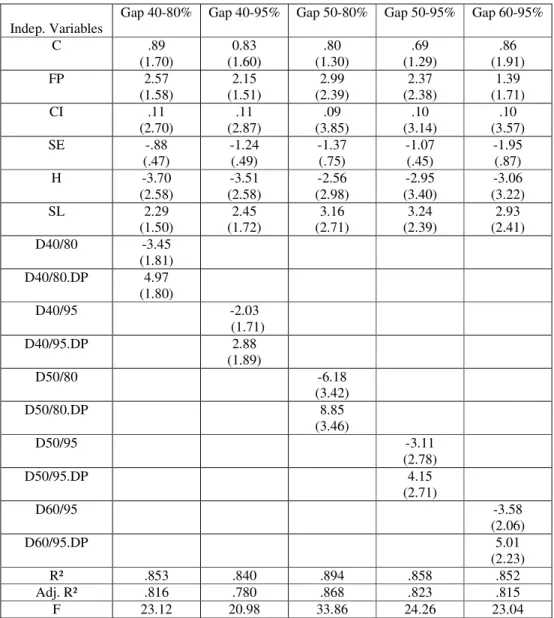
Table 4 shows the results for the different ranges tried. The domestic
performance variables within a lower bound of 40 per cent are not significant, signaling
that the gap cannot be too high. The best results occur for the 50-80 per cent range,
where the cross-product coefficient (β7) has a higher impact, as well as displaying the
highest t-value. We keep this range for further specifications of the model.
It must however be pointed that the 50-80 per cent range, being a data-driven
finding, should not be taken as an “optimal range”, even for the Portuguese reality.
What this exercise confirms is the key role of the gap range for ensuring the occurrence
of spillovers5.
4. DO SPILLOVERS DIFFER BY SECTOR ?
In the previous specifications the vector of parameters β is assumed constant
reasonable because its values are quite differentiated along the sectors. Basic statistics
(see Table 2) show a sector with a highly significant weight of foreign affiliates (sector
38, which includes machinery and transport equipment), two with a low weight (sectors
33, wood and cork, and 37, basic metallurgy), and the remaining ones with values for
foreign presence around the global average.
Table 4.Testing alternative ranges for the technological gap
Indep. Variables
Gap 40-80% Gap 40-95% Gap 50-80% Gap 50-95% Gap 60-95%
C .89 (1.70) 0.83 (1.60) .80 (1.30) .69 (1.29) .86 (1.91) FP 2.57 (1.58) 2.15 (1.51) 2.99 (2.39) 2.37 (2.38) 1.39 (1.71) CI .11 (2.70) .11 (2.87) .09 (3.85) .10 (3.14) .10 (3.57) SE -.88 (.47) -1.24 (.49) -1.37 (.75) -1.07 (.45) -1.95 (.87) H -3.70 (2.58) -3.51 (2.58) -2.56 (2.98) -2.95 (3.40) -3.06 (3.22) SL 2.29 (1.50) 2.45 (1.72) 3.16 (2.71) 3.24 (2.39) 2.93 (2.41) D40/80 -3.45 (1.81) D40/80.DP 4.97 (1.80) D40/95 -2.03 (1.71) D40/95.DP 2.88 (1.89) D50/80 -6.18 (3.42) D50/80.DP 8.85 (3.46) D50/95 -3.11 (2.78) D50/95.DP 4.15 (2.71) D60/95 -3.58 (2.06) D60/95.DP 5.01 (2.23)
R² .853 .840 .894 .858 .852
Adj. R² .816 .780 .868 .823 .815
F 23.12 20.98 33.86 24.26 23.04
We estimated the influence of foreign presence disaggregating FP in model (4)
according to the above grouping: FP = FP1+ FP2+ FP3 , where FP1 includes only sector
38, FP2 sectors 33 and 37 and FP3 the remaining ones (31, 32, 34, 35, 36 and 39). This
means that, for instance, whenever an observation is related to sector 38, FP2 and FP3
are zero, while FP1 equals the value of foreign presence for the corresponding year. The
resulting model is:
PRODit=α+β1FP1it+β2FP2it+β3FP3it+β4CIit+β5SEit+β6Hit+β7SLit+β8D50/80it
+β9D50/80xGTit+∈it . (5)
Results are shown in Table 5, column (1). We also tried out a different grouping,
including sector 38 in the largest previous group (column (2)). In the first case, only
sector 38 presents positive, significant spillovers, an expected result due to the high
share of foreign presence in it (52.5 on average). The influence of sector 38 is
confirmed in the second grouping.
Beyond interacting in a complex way with the gap, the spillover effect is then
also a function of particular sectoral characteristics. The “global” or general spillover
effects found in many empirical works are simply confounding different sector
dynamics.
5. SECTORAL EFFECTS
It is possible that a myriad of influences on productivity – like those related to
the “software” environment for spillovers mentioned by Kokko, as well as to other
sectoral specifics - are not included in the right-hand-side of our equations. These
missing or unobserved variables can be assumed to express the heterogeneity of the
model states that differences across units can be captured in differences in the constant
term. It can be written as:
PRODit=β1FPit+β2CIit+β3SEit+β4Hit+β5SLit+β6Dit+β7DPxDit+∈it (6)
where ∈it= αi +ηit , with the ηit zero-mean, constant variance shocks uncorrelated
across time and units, and the αibeing the unknown individual effects to be estimated
for each unit (sector) i.
Table 5.Panel data: different groups of sectors for FP
Indep. Variables (1) (2)
C 1.37 (1.53) .79 (1.16) CI .010 (3.92) .09 (3.84) SE -1.75 (.84) -1.40 (.74) H -3.42 (2.93) -2.58 (3.07) SL 3.05 (2.46) 3.17 (2.62) D50/80 -7.10 (2.99) -6.18 (3.29) D50/80DP 9.99 (3.07) 8.85 (3.38) FP38 3.08 (1.83) FP33/37 -1.01 (.16) 3.44 (.61) FP31/32/34/35/ 36/39 .52 (.21) FP31/32/34/35/ 36/38/39 3.03 (1.89)
R² .899 .894
Adj. R² .865 .863
F 25.86 28.55
t-values (between brackets) using White’s heteroscedasticity correction
The individual effects may be either fixed or random. In the latter case, though
the αi must be uncorrelated with the explanatory variables, the errors in (6) will be
correlated within sectors. However, when the random effects model is valid, the fixed
the number of units is small enough, model (6), under the fixed effects assumption, can
be estimated by ordinary least squares with one column for each sectoral dummy.
Moreover, a fixed effects approach makes also sense if one considers that the nine
sectors being studied are a full partition of all manufacturing.
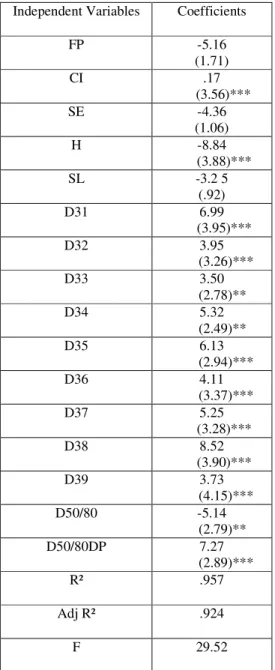
The estimation results are reported in Table 6. It is interesting to compare the
coefficients in this table with those in the related column of Table 4. The four
significant independent variables in the fixed-effects model are as well in Table 4, with
the same signs and, but for the concentration index (H), roughly the same value. Two
major changes then occur for variables FP and SL: their coefficients change sign and
become not significant. On the other hand, all idiosyncratic effects are positive and
significant – most at the 1% level – showing that there clearly exists a sectoral effect.
Indeed, it seems to be more important than those previously accounted for the foreign
presence (FP) and the skilled labor ratio (SL).
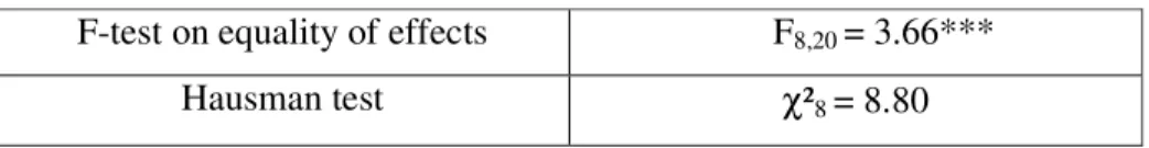
Table 7 presents the results of two tests. The first is a standard F test to check the
null hypothesis that the sectoral effects are all equal. Under this null, the efficient
estimator is pooled least squares, and the ratio:
Fn-1, nT-n-k = [ (R2u-R2r) / (1-R2u) ] x [(nT-n-k) / (n-1)] ,
where u indicates the unrestricted model, r the restricted one, n stands for the number of
units, T for that of periods and k for the number of explanatory variables, is
asymptotically an F. In our case, the corresponding lines in Tables 4 and 6 provide the
R² values for computing the F8,20 statistic. The null is clearly rejected at 1%.
The second is the Hausman test statistic, which tests the null hypothesis that the
(random) effects are uncorrelated with the explanatory variables. Though the null is not
instance, there is not enough variation in the explanatory variables to provide results
precise enough to distinguish between the two sets of estimates (see Johnston and
Dinardo (1997), p. 404).
Table 6.Fixed effects model – least squares estimation
Independent Variables Coefficients
FP -5.16
(1.71)
CI .17
(3.56)***
SE -4.36
(1.06)
H -8.84
(3.88)***
SL -3.2 5
(.92)
D31 6.99
(3.95)***
D32 3.95
(3.26)***
D33 3.50
(2.78)**
D34 5.32
(2.49)**
D35 6.13
(2.94)***
D36 4.11
(3.37)***
D37 5.25
(3.28)***
D38 8.52
(3.90)***
D39 3.73
(4.15)*** D50/80 -5.14
(2.79)** D50/80DP 7.27
(2.89)***
R² .957
Adj R² .924
F 29.52
Table 7.Two tests on the fixed effects model F-test on equality of effects F8,20= 3.66***
Hausman test χ²8= 8.80
The results in this section show that there are significant sector specific effects to
be considered when explaining the productivity variation; the adjusted R2 increases
from 0.868 in Table 4 to 0.924 in Table 6. Moreover, the inclusion of such specificities,
by purging the other coefficients of their effect, apparently changes the empirical role of
foreign presence in the determination of domestic productivity. Combining this with the
result in the previous section raises an important issue: not only the spillover effect
varies with sectors, but due consideration of full sectoral specificities – in a model using
structural characteristics as other explanatory variables – annihilates the global spillover
effect. Two points then ensue. First, dealing with the sectoral dimension requires other
variables than those used so far in the literature. Second, supposing the right variables
are found and included, the “spillovers question” must be reopened. In the remaining of
this paper we will not pursue this line but rather, still at a product market, structural
level, will try to find additional explanations for this key sectoral influence.
6. INTER-SECTORAL SPILLOVERS AND AGGLOMERATION
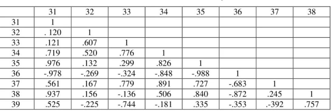
Table 8 shows the correlation coefficients for the residuals in model (2), computed
on a sectoral basis. Given that the residuals account for productivity shocks unexplained
by the model, a high positive correlation would signal a common (hidden) effect on the
two sectors’ productivity. By the same token, high negative correlations would mean
The residuals’ correlations computed from models (2) to (4) show an interesting,
relatively stable pattern. If we consider only those higher than 0.5 in absolute value, all
negative correlations but one are associated with the non-metallic (36) sector, which
opposes five others. Within the positive links, two groups stand out: textiles (32) and
wood and cork (33), both traditional manufactures with a strong historical presence in
the Portuguese economy; and chemicals (35), paper (34), metallurgy (37) and transport
(38), modern sectors with significant market linkages. Food (31) is also worth
mentioning, due to its relevant positive correlation linkages to five sectors.
Table 8.Residuals’ correlations for model (2)
31 32 33 34 35 36 37 38
31 1
32 . 120 1
33 .121 .607 1
34 .719 .520 .776 1
35 .976 .132 .299 .826 1
36 -.978 -.269 -.324 -.848 -.988 1
37 .561 .167 .779 .891 .727 -.683 1
38 .937 .156 -.136 .506 .840 -.872 .245 1 39 .525 -.225 -.744 -.181 .335 -.353 .-392 .757
Given the diversity of goods encompassed by each sector, these results may be
partially due to the high aggregation level of our study, but they also suggest an identity
of reaction to other factors. We venture that such factors might be a combination of
centrifugal and centripetal effects, in the lines of Fujita et al. (1999), responsible for
agglomerations like the one in the Greater Lisbon industrial area, where many of those
firms are located. Agglomeration is viewed here as a matter of external economies of
scale, the hypothesis being that a firm’s profitability increases ifother firmsare nearby.
This could be due either to vertical linkages - i.e., it is advantageous to be near suppliers
knowledge spillovers between firms and indirect knowledge links through a common,
local pool of skilled labor or specialized management, for instance.
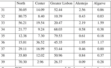
As a way to improve the view on the concentration/spread of sectors outside
Lisbon, Table 9 shows the location of manufacturing activities in the Portuguese
territory in each of the five major regions (NUTS2 level) of the country.
Table 9.Location of manufacturing activities in the Portuguese territorya, 1993
North Center Greater Lisbon Alentejo Algarve 31 30.05 14.09 52.44 2.56 0.86 32 80.75 8.40 10.39 0.43 0.03 33 56.21 19.54 20.47 2.19 1.59 34 21.77 9.24 68.03 0.58 0.38 35 12.38 7.30 79.53 0.61 0.18 36 15.01 36.52 45.35 1.95 1.17 37 29.11 16.99 53.44 0.46 0.00 38 35.80 12.02 50.96 0.84 0.37 39 70.30 2.96 26.37 0.09 0.28
Source: INE a % share of sectoral output
The basic pattern of the correlations is roughly confirmed in both cases, stressing
the economic geography argument. The relative spread of the non-metallic (36) sector,
present in areas where many of the others are barely found; the concentration of
chemicals (35), paper (34), metallurgy (37), transport (38) - and food (31) as well - in
the Greater Lisbon, with a conspicuous presence of chemicals, as expected of a typical
intermediate supplier; the location of the traditional sectors (32 and 33) in the Northern
area, are clear supporting evidences.
Another way to confirm that particular industries are associated with particular
using the production shares in each region. This index provides information on the
extent to which each industry is concentrated in a few regions, but it does not tell
whether these regions are close together or far apart. In fact, using this measure, two
industries may appear equally (geographically) concentrated, while one is roughly
located in two neighboring regions and the other is split among far distant ones. As a
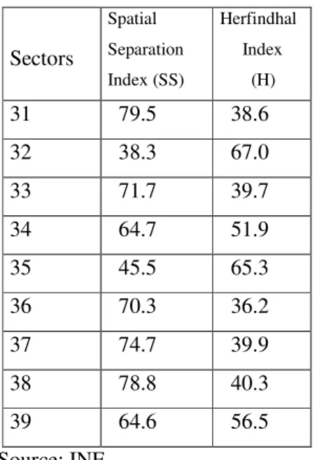
complement to this more traditional concentration measure, the spatial separation index
(SS) proposed in Midelfart-Knarvik et al. (2000), which is a production-weighted sum
of all the bilateral distances between locations (taken as the distance between the most
representative cities in each region), was also computed. If all production occurs in a
single place, SS is zero, and it increases the more spatially separated production is.
The two sets of values in Table 10 suggest, as expected, that regional
concentration roughly decreases as the spatial separation increases. “Non-metallic” is
again worth mentioning, as it is the less concentrated, reasonably spread sector.
Table 10.Spatial location indexes, 1993
Sectors
Spatial Separation Index (SS)
Herfindhal Index
(H)
31 79.5 38.6
32 38.3 67.0
33 71.7 39.7
34 64.7 51.9
35 45.5 65.3
36 70.3 36.2
37 74.7 39.9
38 78.8 40.3
39 64.6 56.5
Further analytical evidence of the influence of the geographical dimension, is
provided by the correlation between the residuals and the Herfindhal spatial
concentration index. Table 11 shows the results for models (2), (3), (4) – with the 50/80
range, and (6). Spatial concentration was now computed at the NUTS3 level, which
increases the number of regions to 28. The first three values are surprisingly similar and
all significantly different from zero. However, for the fixed-effects model the
correlation is (statistically) zero. A hidden spatial dimension, related to the
agglomeration pattern of the sectors, seems evident. In models (2), (3) and (4), where no
attention to the sectoral component is given, part of the residuals dispersion isexplained
by the spatial index. Interestingly enough, the correlation is negative, signaling perhaps
that in the more concentrated sectors other factors had already accounted for the
domestic productivity; the standard model we use overemphasizing the role of the
foreign presence. Inclusion of the sector specificities in (6) brings within it this hidden
spatial dimension, and the correlation falls to zero.
Table 11.Correlations between the residuals and the spatial concentration index Models Correlation
(2) -0.411
(3) -0.414
(4) -0.391
(6) 0.021
Overall, on exploratory grounds - given the reduced number of years in our
panel -, the residuals analysis adds interesting notes to the debate. Specific spatial
relations between groups of industries are suggested, and maybe a sharper
advanced, more traditional sectors from more modern ones - is missing. The
aggregation level of the study puts a grain of doubt on the utility and feasibility of
constructing this new explanatory (and likely omitted) variable. On the other hand, the
suggestion of agglomeration effects finds support, in a much larger spatial dimension, in
the preliminary evidence produced by Barrell and Pain (1999) on the concentration of
the stock of US manufacturing FDI in Europe. How to incorporate this in future
spillover models is an open challenge.
7. CONCLUSIONS
Any result on the existence of spillovers as indicated by the foreign presence
effect on the productivity level of domestic enterprises must be cautiously taken. As
pointed out before, the concept of technological spillovers is quite vast and abstract.
Notwithstanding, the analyses in the previous sections have produced a few new
insights.
We confirmed that the relationship between foreign presence and productivity is
a complex one, being only revealed if the proper controls on these two variables are
used. It is possible that, though present, spillovers are sometimes not identified simply
because they are not increasing linearly with the foreign presence. This nonlinearity is
suggested by the fact that a technological gap seems to be a condition for spillovers, but
only within a certain range. We clearly showed this, first by detecting a significant
interaction between these two variables and then by progressively arriving at “an
optimal gap range” for spillovers.
A crucial influence, of a sectoral nature, is present. Indeed, for some sectors,
modern sectors, with large scale-gains and relatively new in the country. However, the
results of the fixed-effects model indicate that other variables are needed to account for
these differences, as also suggested by the residuals analysis. Moreover, productivity
shocks not described by the variables studied show common patterns among the sectors.
Further work should use this information, which calls attention to proximity effects and
the importance of agglomerations for spillovers diffusion.
The results re-stress the interest of analyzing the spillovers of foreign affiliates
with a case study approach, as a way both to complement the findings and to raise new
issues. It is also worth identifying technology spillovers at a more detailed level, using
as dependent variables improvement measures like R&D expenditures, labor skills, cost
of inputs or the managers’ turnover. Work with disaggregated data at the firm level, and
with different sect oral models, would be relevant to confirm these findings, as firms
can be highly heterogeneous in a given two-digit sector.
As regards specification, two further points have been raised. First, modeling
with product market variables and indicators of sector structure seems to have reached
its limits. New explanatory variables, bringing forward the factors markets and the
intersectoral dimensions, for instance, are needed to produce more consistent views.
Second, either with the same model or in a system of equations, when the analysis
comprises a sufficiently big and diversified region as most countries are (even smaller
ones like Portugal), the spatial dimension, in its agglomeration aspects, must also be
considered. These two issues call for more theory before pursuing the empirics, to avoid
a senseless proliferation ofad hocmodels with a marginal contribution to the subject.
Last but not least, as regards Portugal, the evidence is mixed. If, faithful to
spillover effect in the country has not been produced, rather encouraging suggestions
were raised. Further research on them must be pursued along the lines above.
NOTES
1
For a clear and well-documented survey of the preparations for joining the EU and the post-1986 period see chapters 5 and 6 in Mateus (1998).
2
The Inquérito às Empresas Harmonizado is of the responsibility of the Serviço de Estatísticas Estruturais das Empresas, Departamento de Estatísticas das Empresas/ Instituto Nacional de Estatística, INE, Portugal.
3
Standard deviations across years are, in general, rather small, so that the (row) pattern of the means in Table 2 gives a good approximate picture of the data variation by sector, for each variable.
4
A concept that takes into account the combined productivity of the firm when all inputs are included. See Haddad and Harrison (1993) for a firm specific measure of multi-factor productivity.
5
The reader should also note that model (4) does not include DP itself as an independent variable. Though a possible specification, we favoured the one without it to characterise that it is indeed a “new variable” – the gap within a restricted range – which plays a role in the phenomenon this paper tries to explain.
6
See the appropriate chapters in any econometrics textbook as Johnston and Dinardo (1997), or Judge et al. (1985).
7
This is also an asymptotic test to be taken with care, given our sample size.
APPENDIX
General description of the nine manufacturing sectors
31: Food, beverages and tobacco (food)
32: Textiles, clothing and leather goods, including shoes (textiles)
33: Wood, including furniture, and cork (wood)
34: Paper and printing (paper)
35: Chemicals, rubber and plastics (chemicals)
36: Minerals, non-metallic (non metallic)
38: Steel goods, machines and transport material (transport)
39: Other manufactures (other)
REFERENCES
Aitken, B. J. and Harrison, A. E. (1997). Do domestic firms benefit from direct foreign investment ?Mimeo, Columbia University.
Aitken, B. J. and Harrison, A. E. (1999). Do domestic firms benefit from direct foreign investment ? Evidence from Venezuela.American Economic Review,89(3), 605-18. Barrell, R. and Pain, N. (1999). Domestic institutions, agglomerations and foreign direct
investment in Europe.European Economic Review,43, 925-34.
Blomström, M. (1986). Foreign Investment and Productive Efficiency: the Case of Mexico.The Journal of Industrial Economics,35(1), 97-110.
Blomström, M. and Kokko, A. (1998). Multinational corporations and spillovers. Journal of Economic Surveys,12, 247-77.
Blomström, M. and Persson, H. (1983). Foreign investment and spillover efficiency in an underdeveloped economy: evidence from the Mexican manufacturing industry. World Development,11, 493-501.
Blomström, M. and Wolff, E. (1994). Multinational corporations and productivity convergence in Mexico, in W. Baumol, R. Nelson and E. Wolff (eds.),Convergence of Productivity, Cross National Studies and Historical Evidence. Oxford: Oxford University Press. Djankov, S. and Hoekman, B. (2000). Foreign investment and productivity growth in Czech
enterprises.The World Bank Economic Review, 14, 49-71.
Farinha, F. and Mata J. (1996). The impact of foreign direct investment in the Portuguese economy. Working Paper No. 16/96, Bank of Portugal.
Fujita, M., Krugman, P. and Venables, A. J. (1999).The Spatial Economy-Cities, Regions and International Trade. Cambridge, Mass.: The MIT Press.
Görg, H. and Strobl, E. (2001). Multinational companies and productivity spillovers: a meta-analysis.The Economic Journal, 111(475), F723-F739.
Haddad, M. and Harrison, A. E. (1993). Are there positive spillovers from foreign direct investment? Evidence from panel data for Morocco.Journal of Developing Economics, 42, 51-74.
Developing Countries: Micro Patterns of Turnover, Productivity and Market Structure. Oxford: Oxford University Press.
Johnston, J. and Dinardo, J. (1997).Econometric Methods, 4thed. New York: McGraw-Hill. Judge, G. G., Griffiths, W. E., Hill, R. C., Lütkepohl, H. and Lee, T.-C. (1985). The Theory and
Practice of Econometrics, 2nded. New York: John Wiley & Sons.
Kokko, A. (1992).Foreign Direct Investment, Host Country Characteristics, and Spillovers.Ph. D. Thesis, Stockholm School of Economics.
Mansfield, E. and Romeo, A. (1980). Technology transfer to overseas subsidiaries by U.S.-based firms.Quarterly Journal of Economics,95(4), 737-50.
Mateus, A. M. (1998).Economia Portuguesa. Lisboa: Editorial Verbo.
Midelfart-Knarvik, K.H., Overman, H.G., Redding, S. J. and Venables, A. J. (2000). The location of European industry. Report for the Directorate General for Economic and Financial Affairs. Brussels: European Commission.
Rhee, J. W. and Belot, T. (1989). Export catalysts in low-income countries. Working Paper. Washington, D.C.: World Bank.
Santos, V. (1991). Investimento estrangeiro e a eficiência da indústria portuguesa.Estudos de Economia,11(2), 181-201.