ISSN 1546-9239
© 2008 Science Publications
Corresponding Author: Alongkorn Lamom, Faculty of Engineering, Chulalongkorn University, 10330, Thailand
Heuristic Algorithm in Optimal Discrete Structural Designs
Alongkorn Lamom, Thaksin Thepchatri and Wanchai Rivepiboon Faculty of Engineering, Chulalongkorn University, 10330, Thailand
Abstract: This study proposes a Heuristic Algorithm for Material Size Selection (HAMSS). It is developed to handle discrete structural optimization problems. The proposed algorithm (HAMSS), Simulated Annealing Algorithm (SA) and the conventional design algorithm obtained from a structural steel design software are studied with three selected examples. The HAMSS, in fact, is the adaptation from the traditional SA. Although the SA is one of the easiest optimization algorithms available, a huge number of function evaluations deter its use in structural optimizations. To obtain the optimum answers by the SA, possible answers are first generated randomly. Many of these possible answers are rejected because they do not pass the constraints. To effectively handle this problem, the behavior of optimal structural design problems is incorporated into the algorithm. The new proposed algorithm is called the HAMSS. The efficiency comparison between the SA and the HAMSS is illustrated in term of number of finite element analysis cycles. Results from the study show that HAMSS can significantly reduce the number of structural analysis cycles while the optimized efficiency is not different.
Key words: Heuristic algorithm, steel design, optimization algorithm
INTRODUCTION
There are many techniques used to handle structural optimization problem. Deb and Gulati[1] proposed techniques to design truss structures for minimum weight using genetic algorithm. Shan and Huanchun[2] combined two algorithms to handle the discrete optimization of structures. Chen[3] used the SA to place active passive−1
member in truss structures. Szewczyk and Hajela[4] incorporated the SA and counter propagation neural network to perform structural optimization. Benage and Dhingra[5] proposed three strategies in using the SA to solve single and multi-objective structural optimization problems. Chen and Su[6] suggested two methods to improve SA efficiency in optimal structural designs. Although these referenced techniques can be used to handle structural optimization problem, large numbers of finite element analysis are needed to improve the result. The main problems of using huge number of finite element analysis cycles are that many rejected answers are generated. Consequently, a waste of computer time occurs.
Although the SA is a simple and quite easy technique for implementation, there are many function evaluations needed to find optimal answers in structural optimization problems. Since possible answers given by the SA are randomly generated, the percentage of
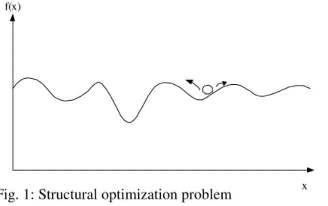
accepted answers is low. Only answers which pass constraint checks are kept. Many generated answers, of course, are rejected because they do not pass constraints. These constraints, known as filters, involve member abilities to support both tension load and compression load. After possible answers are filtered by constraints, the best answer is searched. A typical optimization problem is modeled as shown in Fig. 1.
Theoretically, the probability to generate a new answer at the left hand side and right hand side of the current answer is equal. In structural optimization problems, however, the typical optimized algorithm can be modified to reduce the computation time. In this study, the problem understanding is used to help developing the new algorithm, the HAMSS. Because the structural analysis process spends most of the
Fig. 2: Traveling salesman problem
Cross sectional area Steel volume
Allowable minimum cross sectional area
Fig. 3: Structural optimization problem behavior
computation time in optimization process, the HAMSS will reduce the structural analysis cycles.
Comparison results of the HAMSS, the SA and Multiframe 4D software with three truss examples are presented to demonstrate algorithm’s effectiveness at the end of the paper. The first example is a typical 3 bar planar truss, the second one is a 26 bar planar truss and the last one is a 30 bar curvature planar truss.
HEURISTIC ALGORITHM
Heuristic searching uses knowledge called heuristic to improve the searching efficiency. Heuristic will indicate trend of answers and guide which search route should be better. To show an overview of this method, the classical problem in heuristic algorithm is exampled. The traveling salesman problem is shown in Fig. 2. The objective of this example is to discover the shortest path of salesman’s traveling.
As shown in Fig. 2[7], there are 7 cities. Salesman has to go to all cities and comeback to the started city. The basic method to find the shortest path is generating all routes that is possible, there are (7-1)! 2−1 or 360 routes, then measuring distance of each route. A route
Cross sectional area Steel volume
Allowable minimum cross sectional area Random
Fig. 4: Reducing material size
which has shortest distance is the best solution. However, this method is not practically effective when there are many cities. For example, if 100 cities are goaled, there are 4.67x10155 traveling paths. In this case,
it will take long time to find the optimal answer. A better method to find the shortest path is to use the knowledge of problem understanding to guess the answer. It is obvious that the next selected city for going should be the nearest city. If the every decisions of city selection are nearest city from the current city, the good answer may be investigated. This is an example of using the knowledge to help solving the problem. The selected path may not be the best answer but it is an acceptable one. Using an uncompleted knowledge to handle a problem or a reasonable guessing is called heuristic.
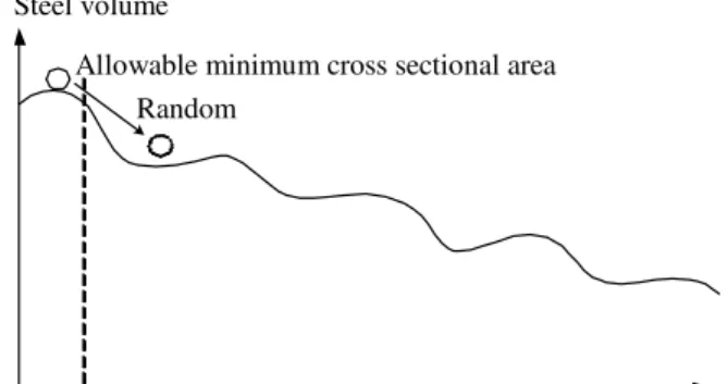
In the SA, although there are many proposed techniques for predicting feasible zone, answers generated for optimal structural problem is randomized. New answers are generated around the present answer as shown in Fig. 1. Each new answer is then checked if it passes all constraints. In this study, behavior of optimal structural problem is studied and is found to be similar to that shown in Fig. 3 with y-axis is the steel volume and x-axis is the cross sectional area of steel in one group. Trend of the best answer occurs at the left hand side of the graph and locates above the load constraint which is converted to be allowable minimum cross sectional area constraint. This constraint varies with steel cross sectional area.
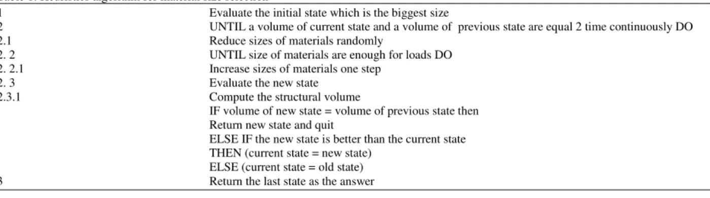
Table 1: Heuristics algorithm for material size selection
1 Evaluate the initial state which is the biggest size
2 UNTIL a volume of current state and a volume of previous state are equal 2 time continuously DO 2.1 Reduce sizes of materials randomly
2. 2 UNTIL size of materials are enough for loads DO 2. 2.1 Increase sizes of materials one step
2. 3 Evaluate the new state 2.3.1 Compute the structural volume
IF volume of new state = volume of previous state then Return new state and quit
ELSE IF the new state is better than the current state THEN (current state = new state)
ELSE (current state = old state) 3 Return the last state as the answer
Cross sectional area Steel volume
Allowable minimum cross sectional area
Fig. 5: Increasing material size
Cross sectional area Steel volume
Allowable minimum cross sectional area
Fig. 6: Algorithm stop
HEURISTIC ALGORITHM FOR MATERIAL SIZE SELECTION
Firstly, the maximum size from the given material data is assigned to be the started answer. Then a new answer is randomly created by reducing size of material as shown in Fig. 4. If this material size is below the allowable minimum cross sectional area line, i.e. the size does not pass the load constraints. A new answer is created by increasing material size one step. This
procedure is repeated until corrected size is obtained as shown at Fig. 5. The algorithm will repeat the process until the steel volume of a new answer does not change for 2 times. The last answer is the best result as shown in Fig. 6.
The Heuristic Algorithm for Material Size Selection is shown in Table 1. Step 1, all members in a structure are assigned to be the biggest size. Step 2 is the stopping evaluation. If the steel volume of the new answer is repeated twice, the algorithm will stop and the last best answer is a final result.In case that the steel volume can be reduced, Step 2.1 will operate. All member sizes are reduced randomly in this step. Members having the same group number, however, will have the same size. Next step is the constraint examination. In step 2.2, all members are verified if their sizes are large enough for load constraints. If material size of any member group is unacceptable, material size of that member group is increased one size at step 2.2.1 until all member sizes pass the load constraints. In step 2.3, the new answer is evaluated. If the new answer is better than the previous one, the current answer is replaced by the new answer. If the new answer is equal to the current answer, the new answer is assigned to be an initial answer for the next loop. These processes at step 2 are recursively operated until the constraint at step 2 is qualified. Then, the last best answer is set to be the final result.
NUMERICAL EXAMPLE
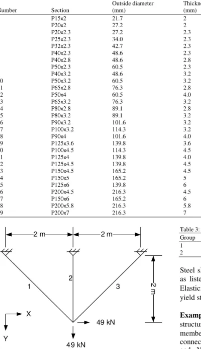
Table 2: Hollow round steel
Outside diameter Thickness Radius of
Number Section (mm) (mm) Area (m2) gyration (mm)
1 P15x2 21.7 2 0.000124 7
2 P20x2 27.2 2 0.000158 8.9
3 P20x2.3 27.2 2.3 0.000180 8.8
4 P25x2.3 34.0 2.3 0.000229 11.2
5 P32x2.3 42.7 2.3 0.000292 14.3
6 P40x2.3 48.6 2.3 0.000335 16.4
7 P40x2.8 48.6 2.8 0.000403 16.2
8 P50x2.3 60.5 2.3 0.000421 20.6
9 P40x3.2 48.6 3.2 0.000456 16.1
10 P50x3.2 60.5 3.2 0.000576 20.3
11 P65x2.8 76.3 2.8 0.000647 26
12 P50x4 60.5 4.0 0.000710 20
13 P65x3.2 76.3 3.2 0.000735 25.6
14 P80x2.8 89.1 2.8 0.000759 30.5
15 P80x3.2 89.1 3.2 0.000864 30.4
16 P90x3.2 101.6 3.2 0.000989 34.8
17 P100x3.2 114.3 3.2 0.001117 39.3
18 P90x4 101.6 4.0 0.001226 34.5
19 P125x3.6 139.8 3.6 0.001540 48.2
20 P100x4.5 114.3 4.5 0.001552 38.9
21 P125x4 139.8 4.0 0.001707 48
22 P125x4.5 139.8 4.5 0.001913 47.9
23 P150x4.5 165.2 4.5 0.002272 56.8
24 P150x5 165.2 5 0.002516 56.7
25 P125x6 139.8 6 0.002522 47.4
26 P200x4.5 216.3 4.5 0.002994 74.9
27 P150x6 165.2 6 0.003001 56.3
28 P200x5.8 216.3 5.8 0.003836 74.5
29 P200x7 216.3 7 0.004603 74
2 m 2 m
2
m
49 kN
4 9 kN 1
2
3
X
Y
Fig. 7: A 3 bar planar truss (Example 1)
(HAMSS). These algorithms are implemented in SUTStructure[9,10]. SUT structor is an education structural analysis software used to analyze two dimensional truss and frame structures. Structural design criteria used in the Multiframe and the SA is the Allowable Stress Design (ASD) given in the AISC 1989 specification. The HAMSS algorithm however uses the ASD from both the AISC 1989 and AISC 2005 specifications[11].
Table 3: Group information (Example 1)
Group Members
1 1, 3
2 2
Steel shape used in the study is the hollow round steel as listed in Table 2. There are 29 sizes. Modulus of Elasticity, E, is 196x106 kN m−2 (2x10¹⁰ kg m2) and yield stress, Fy, is 245000 kN m−2
(25000000 kg m−2 ).
Example 1: The first example is a typical planar truss structure. The structure is a 3 bar planar truss. All members in the structure are connected by hinged connections. Load 49 kN (5000 kg) acts along both X and Y-axis as shown in Fig. 7. Material group information is given in Table 3. Materials sizes are divided into 2 groups. Material sizes of member 1 and member 3 are equal and assigned to be group 1 while member 2 is different and assigned to be group 2.
Table 4: Results from algorithms (Example 1)
Multiframe SA HAMSS HAMSS
Group (ASD1989) (ASD1989) (ASD1989) (ASD2005)
1 P40x2.8 P40x2.8 P40x2.8 P40x2.8
2 P15x2 P15x2 P15x2 P15x2
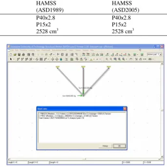
Volume 2528 cm3 2528 cm3 2528 cm3 2528 cm3
0.000 0.005 0.010 0.015 0.020 0.025 0.030 0.035 0.040
0 50 100 150 200 250
Number of finite element analyses All answers Accepted Answers Steel volume ( m3)
Fig. 8: Convergent graph of the SA (Example 1)
0.000 0.005 0.010 0.015 0.020 0.025
0 5 10 15 20
Number of finite element analyses All answers
accepted answers
Steel volume ( m3)
Fig. 9: Convergent graph of the HAMSS (Example 1)
Fig. 10: Results from the implemented program (Example 1)
biggest steel size in each group is selected to be the selected size of that group. From the study, the optimum steel volume of the structure is 2528 cm3. Selected steel sizes are shown in Table 4.
In the SA, the design criteria used with this algorithm is based on the AISC 1989. The example is run with this algorithm for 25 times. The best design from these results is selected to be the answer. To obtain the optimal answer, the SA uses 196 finite element analyses. The optimum steel volume of the structure designed by the SA is 2528 cm3. Selected steel sizes are listed in Table 3. The intermediated results from log file are plotted as convergent graph in Fig. 8. It should be noted that both the Multiframe and the SA algorithm yield the same optimum steel volume.
In the HAMSS, both AISC 1989 and AISC 2005 (ASD) are studied. The example is tested with this algorithm for 25 times. The optimum steel volume of the structure designed by the HAMSS with both AISC 1989−1
and AISC 2005−1
Fig. 11: A 26 bar planar truss (Example 2)
Table 5: Group information (Example 2)
Group Members
1 1, 5, 6-10, 11-16
2 2, 3, 4
3 17-20, 23-26
4 21, 22
0.00 0.05 0.10 0.15 0.20 0.25 0.30
0 200 400 600 800
Number of finite element analyses All answers
Accepted answers Steel volume(m3
)
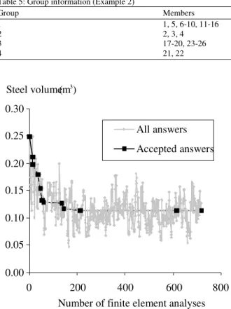
Fig. 12. Convergent graph of the SA (Example 2)
HAMSS required only 16 finite element analyses when compares to 269 finite element analyses used in the SA. Table 4 reports steel volume and selected steel sizes designed by the Multiframe, the SA and the HSMSS algorithms. All design techniques give the same results. However, it should be pointed out that the
Example 2: The second example is a 26 bar planar truss with joint loads as shown in Fig. 11. All connections in the structure are hinged connections. The truss is also pin supported at both ends. The structure is 1.5 m high and 10 m long.
Material sizes in the structure are assigned into 4 groups. Information of members using the same steel size is shown in Table 5.
The steel volume of the structure obtained from the Multiframe is 103289 cm3. The selected steel sizes are shown in Table 6.
In the SA, the example is run with this algorithm for 25 times. The best design from these results is selected to be the answer. Fig. 12 shows convergent performance of the SA. To find the optimal answer in this example, the SA requires 719 finite element analyses. The optimum steel volume of the structure designed by the SA is 112785 cm3. Selected steel sizes are shown in Table 6. According to the information in Fig. 12, it can be seen that many answers are generated but they are mostly rejected. Most of them do not pass steel design criteria. Many rejections cause much
Table 6: Results from algorithms (Example 2)
Multiframe SA HAMSS HAMSS
Group (ASD1989) (ASD1989) (ASD1989) (ASD2005)
1 P100x3.2 P125x4.5 P80x3.2 P90x3.2
2 P200x7 P200x5.8 P200x7 P200x5.8
3 P125x3.6 P125x3.6 P100x3.2 P100x3.2
4 P200x5.8 P200x4.5 P200x5.8 P200x4.5
0 0. 02 0. 04 0. 06 0. 08 0. 1 0. 12 0. 14 0. 16
0 5 10 15 20 25
Num ber of finit e elem ent analyses All answers
Accepted answers St eel volum e (m3)
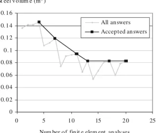
Fig. 13: Convergent graph of the HAMSS (Example 2)
Fig. 14: Results from the implemented program (Example 2)
Table 7: Group information (Example 3)
Group Members
1 1-7
2 8-14
3 15-22
4 23-25, 28-30
5 26, 27
0.00 0.10 0.20 0.30 0.40 0.50 0.60
0 200 400 600 800 1000
Number of finite element analyses All answers
Accepted answers Steel volume (m3)
Fig. 15: Convergent graph of the SA (Example 3)
computation time for answer validations. These times are totally waste.
In the HAMSS, The optimum steel volume of the structure designed using the ASD 1989 standard is 89010 cm3 and it requires only 20 finite element analyses. Also in the HAMSS with ASD 2005, the optimum steel volume of the structure is 83073 cm3 and it spends only 20 finite element analyses to get the answer. These results show that the HAMSS is more powerful than the SA in term of number of finite element analyses. The convergent performance graph of HAMSS for the ASD 2005 version is shown in Fig. 13. Only 14 rejected answers are created. The final results reported from the implemented program are presented in Fig. 14.
Table 6 shows the optimum structural steel volume and selected material sizes designed by each technique.
According to information in Table 6, the optimum steel volumes of the structure designed using both versions of the HAMSS, AISC 1989−
and AISC 2005−1 , are also significantly better than the optimum steel volume of the structure designed using the Multiframe and the SA.
Table 8: Result from algorithms (Example 3)
Multiframe SA HAMSS HAMSS
Group (ASD1989) (ASD1989) (ASD1989) (ASD2005)
1 P200x4.5 P150x6 P200x4.5 P200x4.5
2 P125x3.6 P125x3.6 P125x3.6 P125x3.6
3 P65x3.2 P80x2.8 P65x3.2 P65x3.2
4 P65x2.8 P40x3.2 P40x3.2 P40x3.2
5 P90x3.2 P80x2.8 P80x2.8 P80x2.8
0.00 0.05 0.10 0.15 0.20 0.25 0.30 0.35
0 10 20 30
Number of finite element analyses All answer
Accepted answers Steel volume ( m3)
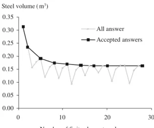
Fig. 16: Convergent graph of the HAMSS (Example 3)
Example 3: The third example is a 30 bar planar truss with joint loads as shown in Fig. 15. The structure is 5.5 m high and 28 m long. The structure is pin supported at both ends. All connections in the structure are hinged connections. Material sizes in the structure are assigned into 5 groups. Members that use the same steel size are grouped and shown in Table 7.
The example is computed by the Multiframe software, the SA and both versions of the HAMSS. The optimum steel volume of the structure designed by the Multiframe is 169277 cm3. Selected steel sizes are shown in Table 8.
In the SA, the design criteria used with this algorithm is based on the AISC 1989. The example is run with this algorithm for 25 times. The best design from these results is selected to be the answer. To obtain the optimal answer, the SA uses 829 finite element analyses. The optimum steel volume of the structure designed by the SA is 162485 cm3. Selected steel sizes are listed in Table 8. The intermediated results from log file are plotted as convergent graph in Fig. 13. The dark points are the accepted answers and the gray points are the rejected answers. This information show that the SA can find the optimal solution, but many waste answers are created before the best answer is found. Most answers are rejected because either the answers do not pass the constraints or the answers are not better than the previous answer.
In the HAMSS, both AISC 1989 and AISC 2005 (ASD) are studied. The optimum steel volume of the structure which is designed by the HAMSS with both AISC 1989−1 and AISC 2005−1 (ASD) is 162485 cm3. The intermediated results from the HAMSS for AISC 2005 (ASD) standard are graphically shown in Fig. 16.
It should be noted that the number of finite element analyses in Fig. 16 is less than the number of finite element analyses in Fig. 15. Final results reported from the implemented program based on HAMSS (AISC 2005−1) is shown in Fig. 17.
Table 8 shows the optimum structural steel volume and selected material size designed by each technique.
Fig. 17: Results from the implemented program (Example 3)
From the study, the optimum steel volumes of the structure designed by both versions of the HAMSS are better than the SA. In addition, the HAMSS with AISC 2005 specifications requires only 28 finite element analyses when compares to 829 analyses used in the SA.
DISCUSSION
efficient optimization technique which is easy for understanding and simple for implementation.
In the future, the HAMSS would be used to solve other problems which are similar to the optimal discrete structural design problem. The other types of structural material and other types of structure will be tested with HAMSS.
REFERENCES
1. Kalyanmoy, D. and S. Gulati, 2001. Design of truss-structures for minimum weight using genetic algorithms. Finite element in analysis and design, 37: 447-465.
2. Chai, S. and S. Huanchun, 1997. A combinatorial algorithm for the discrete optimization of structures. Appl. Math. and mech., 18: 847-856. 3. Chen, G.S., R.J. Bruno and M. Salama, 1991.
Optimal placement of active passive−1 members in truss structures using simulated annealing. AIAA, 29: 1327-1334.
4. Szewczyk, Z. and P. Hajela, 1993. Neural network approximation in a simulated annealing based optimal structural design. Structural and Multidisciplinary Optimization, 5: 159-165.
5. Bennage, W.A. and A.K. Dhingra, 1995. Single and multiobjective structural optimization in discrete-continuous variables using simulated annealing. Int. J. Numerical Method in Eng., 38: 2753-2773.
6. Ting-Yu, C. and S. Jyh-Jye, 2002. Efficiency improvement of simulated annealing in optimal structural designs. Advances in Eng. Software, 33: 675-680.
7. Boonserm, K., 2003. Artificial Intelligence, pp: 16-17.
8. Formation Design Systems. Multiframe4D, http://www.formsys.com/multiframe
9. Alongkorn, L. and T. Bisarnsin, 2002. Structural Analysis Software for Education in Proceeding of the 8th National convention on civil engineering, Thailand, pp: 119-123.
10. Alongkorn, L. and W. Rivepiboon, 2005. A Nodal Numbering Algorithm for 2D Structural Simulation. ECTI Transactions on Computer and Information Tech., 1: 108-116.