IMPROVED ALGORITHM FOR ROAD REGION SEGMENTATION BASED ON SEQUENTIAL MONTE-CARLO ESTIMATION

Natarajan Meghanathan et al. (Eds) : WiMONe, NCS, SPM, CSEIT - 2014

pp. 171–183, 2014. © CS & IT-CSCP 2014 DOI : 10.5121/csit.2014.41213

Zdenek Prochazka

Department of Information Engineering,

National Institute of Technology, Oita College, Oita, Japan

zdenek_p@oita-ct.ac.jp

ABSTRACT

In recent years, many researchers and car makers put a lot of intensive effort into development of autonomous driving systems. Since visual information is the main modality used by human driver, a camera mounted on moving platform is very important kind of sensor, and various computer vision algorithms to handle vehicle surrounding situation are under intensive research. Our final goal is to develop a vision based lane detection system with ability to handle various types of road shapes, working on both structured and unstructured roads, ideally under presence of shadows. This paper presents a modified road region segmentation algorithm based on sequential Monte-Carlo estimation. Detailed description of the algorithm is given, and evaluation results show that the proposed algorithm outperforms the segmentation algorithm developed as a part of our previous work, as well as an conventional algorithm based on colour histogram.

KEYWORDS

Lane Recognition, Road Region Segmentation, Sequential Monte-Carlo Estimation

1.

I

NTRODUCTION

In recent years, many car makers put a lot of intensive effort into development of autonomous driving systems, and published their plans to start production of cars with self-driving ability within next few years.

Autonomous driving systems exploit information from various sensors, and interpret sensory information to identify appropriate navigation paths, as well as obstacles and relevant signage. Among various sensors, a camera is an indispensable one, because real human driver rely mainly on visual information, and transport infrastructure is most suited to the human vision system.

The development of computer vision techniques for autonomous driving is a very challenging task, and intensive research on this topic is carried out. Our work deals with an issue of computer vision based lane detection.

however it can easily fail if road boundaries are not clear, or if strong edges caused by non-road objects are present in image. It is also not obvious, how to handle complicated road shapes, splitting and merging of traffic line, complicated road marking, or sudden changes in road width.

To overcome the limitations of the boundary based approach, techniques for segmentation of road as a region are intensively studied. A common issue with the road region segmentation is how to build a classifier to make decision whether a image pixel belongs to the road surface or not. There are two basic approaches to this issue. The first one is adopting an algorithm from field of machine learning. Methods based on neural networks [6] or SVM [7,8] are reported. Since the training of the classifier is generally an off-line process, the main difficulty with such kind of methods is how to bring adaptability to new data which appear during detection stage and were not part of the original training set.

The second approach are methods based on idea of statistical decision. Statistical distribution of road features is modelled as parametric or non-parametric probability distribution function (pdf), and the pdf is used to decide whether a given image pixel is part of road or not. Methods using simple Gaussian colour model [9], Gaussian mixture model [10], histogram of colour components [11], histogram of illumination invariant features [12] have been reported. The main difficulty with the methods based on statistical decision is the fact, that it is not obvious how to estimate pdf. To estimate pdf for each incoming frame, we need to some guess where the road is, which can easily pose a chicken and egg problem. In many cases, some simple heuristics or ad-hoc solutions are adopted. Furthermore, although the road segmentation should be performed over an sequential image, many of the developed methods study segmentation only from single frame of road image, and behaviour for image sequence is not studied enough.

In our work, we have focused to approach of statistical decision, and attempt to solve estimation of pdf for sequential image in more systematic way. In our previous report, we have already proposed a road segmentation algorithm based on sequential Monte-Carlo (SMC) estimation [13], and applied it to region-based pathway estimation [14]. Although this segmentation method yields better results than the conventional one, and it is quite robust to parameter setting, it still doesn’t produce optimal result under certain circumstances. This paper shows a limitation of the original algorithm and presents a new algorithm with improved segmentation ability. The proposed algorithm is based upon a sound theoretical framework, and evaluation results for various kinds of image data are shown to demonstrate effectiveness of our proposal.

Although an issue of shadows is not discussed in this paper, it should be mentioned that the proposed method can be easily adapted to other type of features, which are claimed to be less sensitive to illumination [10,12].

This document describes, and is written to conform to, author guidelines for the journals of AIRCC series. It is prepared in Microsoft Word as a .doc document. Although other means of preparation are acceptable, final, camera-ready versions must conform to this layout. Microsoft Word terminology is used where appropriate in this document. Although formatting instructions may often appear daunting, the simplest approach is to use this template and insert headings and text into it as appropriate.

2.

SMC

E

STIMATION

E

ASED

R

OAD

S

EGMENTATION

A

LGORITHM

2.1. Former Algorithm

Let f be a vector of road features. In this work, a five dimensional feature vector f =

is used, where

f

₁ and f₂ corresponds to pixel coordinates xandy respectively, and f₃, f₄,f₅ corresponds to colour components r,g,b. Although r,g,b were adopted, the algorithm is generally not limited to these features. For convenience we define also vectors

T T

f f y

x, ) ( , )

( = _{1 2}

=

x and c=(r,g,b)T =(f₃,f₄,f₅)Tas shorthand for vector of coordinates and colour components respectively. With this notation, the feature vector can be expressed also as f =(xT,cT)T.

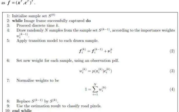
Figure 1. Original Algorithm

The goal is to estimate pdf of road features p(f), and use the estimated pdf to classify road and non-road pixels. Since the road can take various shapes, p(f) is expected to be a non-Gaussian distribution at least with respect to the x. This suggests that we need an estimation method which can handle general type of distribution. Since the road usually looks very similar between two successive frames, and overall visual appearance changes relatively slowly compared to frame rate, temporal continuity can be involved into the pdf estimation, and it should be possible to model a visual changes of road as a stochastic process.

Taking the above mentioned into account, we have focused to SMC (Sequential Monte-Carlo) estimation as a basic tool for estimation of the p ( f ). The original segmentation algorithm was inspired by CONDENSATION algorithm [15]. The pdf is expressed in discrete form as a set of weighted samples S ,

where f_i is a sample of the feature vector f and w_i is an importance weight assigned to the sample. Estimation is performed by repetitive update of the S according to the algorithm shown in Figure 1. The superscript k stands for discrete time here. The in the eq.(2) means a vector of Gaussian random numbers with zero mean and variances

σ

₁,Λ

σ

₅ . The p(z_i|c_i) in eq.(3) is an observation pdf defined by eq.(5).

(a) Original Image (b) Samples (c) Segmentation Result

Figure 2: Example of Segmentation Result

= − − Σ− −

) ( ) ( 2 1 exp ) |

( _{i i i i} T _m1 _{i i}

p z c c z c z (5)

The symbol Σ_m here means a diagonal matrix of variances, controlling width of exponential function for each colour component, and z_i means a colour component observed at position

obtained from eq.(2). Simply said, the p(z_i|c_i) is a measure of similarity between colour components c_i predicted by eq.(2), and colour components observed at predicted positions. The calculated similarity is than assigned as an importance weight.

The above described algorithm estimates the pdf in a form of weighted samples. To evaluate pdf for an arbitrary pixel, we perform a smoothing of the estimated pdf, in a way similar to non-parametric density estimation, using kernel function

φ

. Hence, the pdf p(f) for an arbitrary pixel values f is calculated as

= = N i i i w p 1 ) , ( )

(f

φ

f f (6)

= − − Σ− −

) ( ) ( 2 1 exp ) ,

(f f_i

β

f f_i T _s1 f f_i

φ

where the symbol Σ_s is a diagonal matrix of parameters, controlling window width for each component of f , and the

β

is a normalising constant. Segmentation of the road region is performed by evaluation of p(f) for each pixel, followed by thresholding of obtained values to decide road and non-road pixels.

The image shown in Figure 2(a) is a synthetic image, and the road region can be segmented very easily here.The Figure 2(b) shows a spatial distribution of samples f_i, after the method described above has been applied. As can be seen, the samples are not distributed uniformly, and only few samples appear over left and right side of low part of the road region. As a consequence, these parts are not segmented properly, as is shown in Figure 2(c). Such improper distribution of samples can cause serious problems in proper segmentation of roads with multiple traffic lines.

There is another issue, which can’t be simply shown by static image. Since the estimation of pdf of the road features is treated as an stochastic process, certain noise has to be introduced into the model. Due to this stochastic nature, the positions of samples change between subsequent frames, and segmented parts of road covered only by few of samples are very sensitive to such changes. Due to this, rapid changes in shape of the segmented road appear from frame to frame, although the road doesn’t changes significantly in the image. We refer these quick temporal changes of segmentation result as fluctuations in the following. It is clearly an unwelcome phenomenon which have to be eliminated.

After careful revision of the original algorithm, we have proposed a new algorithm, which attempts to solve the above mentioned issues.

2.2. Proposed Algorithm

The limitations of the original algorithm are caused by improper distribution of the samples during the estimation process. To obtain proper segmentation result, samples should be spread uniformly over the road region, and the sampling method described in step 4 of the Figure 1 can’t guarantee this property. In the original algorithm, the only way to spread samples more widely over the road region is to increase amount of transition noise added to spatial components. However this cause larger fluctuations of the segmented region, therefore limitations of the original algorithm cannot be simply solved by parameter tuning.

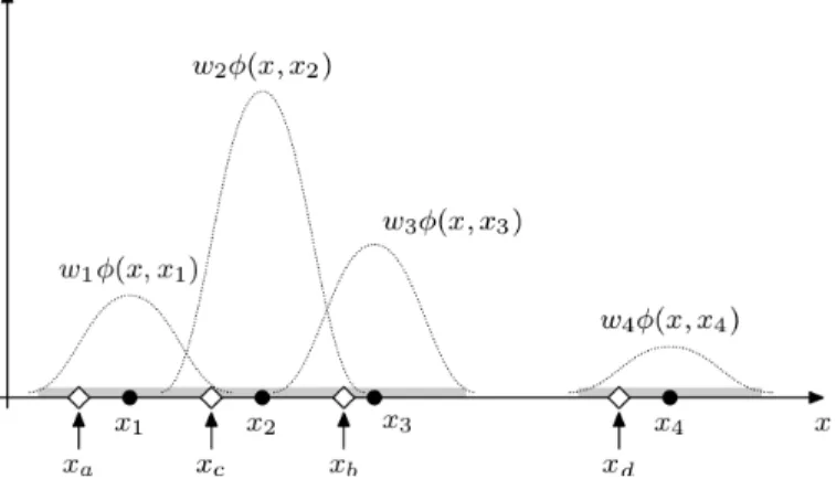
Figure 3: Assignment Between Subsequent Samples

Our idea to solve discussed issues is based on the principle of importance sampling [17]. In this framework, it is supposed that samples can be easily drawn from some probability distribution

) , | ( ) | ( ) | ( ) ( ) 1 ( ) ( ) 1 ( ) ( ) 1 ( ) ( ) 1 ( ) ( k k i k i k i k i k i k k i k i q p p w w z f f f f f z − − − −

∝ (7)

Although principle of importance density provides sound theoretical framework, the specific

forms of p(z(k)| f_i(k−1)) , p(f_i(k)| f_i(k−1)) and q(f_i(k)| f_i(−1),z_i(k)) are not obvious, and strongly depends on particular application.

In our case, we have chosen q(f_i(k)| f_i(−1),z_i(k)) as a uniform distribution with respect to spatial components x , where the range of x is limited to region segmented at the previous time step. Simply said, spatial components of the generated samples x_i (i=1,Λ ,N) are uniformly drawn from the region obtained at k−1.

To evaluate ( ( )| (k−1)) i k i

p f f , we need to establish relations between old samples and new samples generated according to importance density. This is not straightforward, and our idea is to perform assignment in a way described in Figure 3 for single variate case. Let the x₁,Λ,x₄ be old samples, and let the intervals highlighted by light grey be segmented parts of x axis. We draw new samples from the light grey intervals randomly, according to a uniform distribution. New samples are shown by diamond and the alphabet subscript here. For each new sample

i

x (i=a,b,c,d) we assign one of the old samples x_j (j=1,2,3,4), using the weighted kernel function

φ

, already mentioned in eq.(6), as an assignment criteria.

arg max( ( , )) 4

, ,

1 j x i j j w x x

l

φ

Λ =

= (8)

Here,

φ

_x stands for univariate Gaussian kernel function. The l obtained by eq.(8) is than used as a subscript of assigned old sample. For the situation in Figure 3, the resulting assignment is

) ,

(x_a x₁ , (x_b,x₃), (x_c,x₂), (x_d,x₄).

We have described the basic idea of sample assignment for simple univariate case. Next we explain, how to extend this idea to the our case of f . Since our importance density is defined in spatial subdomain x, we perform assignment of samples with respect to x. Therefore, after the new samples x_i(k) are generated according to importance density, we assign to each generated

sample an old one, for which the ( −1)

(

( ), (k−1)

)

j k i k j

w

φ

_x x x is maximal. The symbol

φ

_x here stands for kernel function of the same form as in eq.(6), however applied only to spatial components .

By the above described procedure, we can generate spatial part x_i(k) of the new samples, and perform assignment between new and old samples. However, we said nothing about the colour part c_i(k) so far. To generate colour part of the new samples, and build up complete samples

) (k i

f , we simply apply transition equation to colour part of assigned old sample.

c_i(k) =c_l(k−1)+_{c i}

(9)

After the new sample set f_i(k) is completed, we evaluate transition pdf in weight update equation as

( ( )| ( −1))= ( ( )| (k−1)) l k i k

l k i

p f f

φ

f f (10)

where

φ

has a same form as in eq.(6), andl is a label of sample assigned to the i-th one.

The last component needed for weight update calculation in eq.(7) is the observation pdf )

| ( (k) _i(k−1)

p z f , and it has the same form as was already shown by eq.(5).

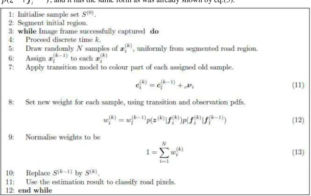
Figure 4. Proposed Algorithm

The proposed algorithm is summarised in Figure 4.In the weight update eq.(12) of the step 8, the value of importance density q is omitted, since we draw samples according to uniform distribution.

At the end of this section, we show a simple example of the segmentation result obtained by the proposed algorithm. The result for the same data as in Figure 2 is shown in Figure 5. As can be seen, samples are spread over all road region and there are no missing parts of segmented road region.

In the next section, we present more detailed evaluation of the proposed algorithm for various kinds of image data.

3.

E

VALUATIONOF

T

HE

P

ROPOSED

A

LGORITHM

The evaluation of the proposed algorithm have been performed on the following kinds of image data.

A: Sequences of Still Images

Approximately 200 images, capturing frontal roads viewed from car, were randomly collected. Half of them are structured roads, second half are unstructured and rural roads. For the each image, a sequential image was created by repeating of the same still image. Created sequential images shows snapshots of real road, but since there are no temporal changes between subsequent frames, these data can be used to assess fluctuations of the resulting segmentation.

B: Synthetic Image Sequence

Sequence of rendered CG images, already used in Figure 2 and Figure 5, was created. The sequence simulates a vehicle moving by 60 km/h on road with 4 curves (R=150m, 100m, 80m, 50m). Vehicle steering is simulated by changes in lateral position and pitch angle. Since the sequence is composed of road images with almost homogeneous colour, the perfect segmentation of road region can be done very easily, and this sequence can be used to assess quality of segmentation.

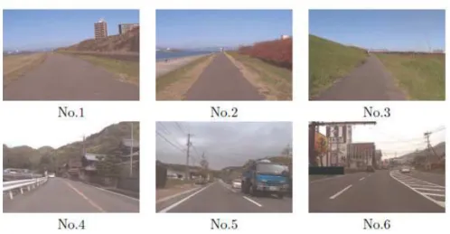
C: Real Image Sequences

Real image sequences, already mentioned in our report [14], with representative frames shown in Figure 6. These sequences are real data, therefore they can be used to assess overall ability of the algorithm.

For all above mentioned data, ideally segmented road regions were prepared as ground truth. The segmentation was done manually for data A and C, and automatically during CG rendering for data B.

As a quantitative measure of the segmentation ability, we adopted Jaccard index J, defined by eq.(14).

| |

| |

g s

g s

R R

R R J

∪ ∩

= (14)

Here, R_sis a set of road pixels obtained by segmentation algorithm, and R_g is a set of road pixels for ground truth. Symbol | | means a set size here. Jaccard index J takes value 1 if both sets R_s

and R_g are identical.

Figure 6: Real Image Sequences

SRG based algorithm use normalised histogram of features as a merging criteria (pixel is merged if histogram value for pixel features is greater than certain threshold). The histogram of features is calculated from region placed over low part of road image. This follows the same strategy as I reports [11] and [12]. Placement of seed points follows suggestions given by report [12].

SRG based algorithm, original SMC based algorithm and proposed SMC based algorithm were evaluated for data A, B, C. Before evaluation, all necessary parameters were once tuned to maximise average value of Jaccard index eq.(14). After tuning, parameter values were fixed, and same fixed values were used for all tested data.

Figure 7: Configuration of SRG Based Reference Algorithm

3.1. Evaluation for Sequences of Still Images

Three mentioned algorithms, were applied to data A, and Jaccard index eq.(14) was calculated for segmentation results of each particular sequence frame by frame. Next, average

µ

_J and standard

deviation

σ

_J of Jaccard index was calculated separately for each sequence, and these values were

used to form histograms of

µ

_J and

σ

_J respectively. The resulting histograms are shown in Figure 8. Since data A have no temporal changes, results by SRG based algorithm contains no fluctuations, and evaluation of

σ

_J has no meaning for data A. Therefore, only result for SMC

ideal value

µ

_J =1, and (b) of the same figure shows that peak of histogram for the proposed algorithm is closer to ideal value

σ

_J =0. It means, that for majority of the data A, the proposed algorithm yields segmentation results closer to ground truth, while fluctuations of segmented regions are reduced. The result for SRG based algorithm is surprisingly wrong. The values of average of Jaccard index are distributed in wide range, which shows that the SRG based algorithm is not robust to parameter setting.

(a) Histogram of Means

µ

_J (b) Histogram of Standard Deviations

σ

_J Figure 8: Histogram of Jaccard Index for Sequences Still Image

3.2. Evaluation for Synthetic Image Sequence

Three mentioned algorithms were applied to data B, and Jaccard index eq.(14) was calculated for each segmented frame of image sequence. Graphs of the Jaccard index are shown in Figure 9. It can be seen, that proposed algorithm yields similar result as SRG based algorithm, where result in Figure 9(a) is more noisy than Figure 9(c). This is caused by fact, that SRG based algorithm segments each frame as an independent still frame and there is no mechanism for temporal continuity. The result for original algorithm in Figure 9(b) contains large fluctuations, and magnitude of fluctuations is significantly reduced by the proposed algorithm.

(a) SRG Based (b) SMC Based Original (c) SMC Based Proposed

Figure 9: Jaccard Index for Synthetic Image Sequence

3.3. Evaluation for Real Image Sequences

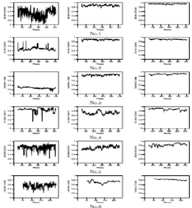
issue discussed in subsection 2.1, other traffic lines are not segmented properly. The proposed algorithm shows lower magnitude of fluctuations and overall shows high values of J. Several decreases of J can be observed in sequence No.5. Let us now look more closely on segmentation results fore such frames. Figure 11

(a) SRG Based (b) SMC Based Original (c) SMC Based Proposed

Figure 10: Jaccard Indexes for Real Image Sequence

shows result for frame 125 of sequence No.5. This is a situation immediately after another car has passed an opposite traffic line. Since samples disappear from road parts occluded by passing car, these parts are not segmented, and a few iterations of the algorithm are needed to spread samples over the previously occluded road parts. Due to this the Jaccard index decreases for few frames, because the segmented region differs from its ground truth.

The evaluation results for data A, B, C described above shows, that the proposed algorithm pose an effective solution to the issues discussed in subsection 2.1.

4. C

ONCLUSION

A

ND

F

URTHER

W

ORK

This paper has presented a road segmentation algorithm based on sequential Monte-Carlo estimation. The proposed algorithm is an extension of our previous work on topic of road region segmentation, and the proposed algorithm solves issues remained in original SMC based segmentation algorithm.

The key idea of the proposed algorithm lies in improvement of sampling method and consequent calculation method of importance weights. Drawing samples according to distribution of importance weights, which was adopted in the original algorithm, was not optimal for road region segmentation, and more general approach based on principle of importance sampling has been introduced. Particularly, uniform sampling from region segmented at previous time step was introduced to generate new sample set, and assignment between subsequent samples was introduced to evaluate transition probability density function required in weight update.

The proposed algorithm was evaluated on three types of image data, and evaluation results shows superiority of the proposed algorithm over the original one, as well as over the algorithm based on seeded region growing.

In the proposed algorithm, RGB colour components were used as features, however the proposed algorithm can be easily adapted to different features too. Evaluation of the proposed algorithm for features which are more resistant to illumination changes, and adaptation of the algorithm for road images with hard-cast shadows is a main direction for future work.

R

EFERENCES

[1] Y. Wang, D. Shen, and E. Teoh, “Lane detection using catmullrom spline,” in IEEE International Conference on Intelligent Vehicles, 1998, pp. 51–57.

[2] B. Ma, S. Lakshmanan, and A. O. Hero, “Pavement boundary detection via circular shape models,” in Proceedings of the IEEE Intelligent Vehicles Symposium 2000, 2000, pp. 644–649.

[3] Y. Wang, E. Teoh, and D. Shen, “Lane detection and tracking using b-snake,” ImageVision and Computing , vol. 22, no. 4, pp. 269–280, Apr. 2004.

[4] H. Xu, X. Wang, H. Huang, K. Wu, and Q. Fang, “A fast and stable lane detection method based on b-spline curve,” in IEEE 10th International Conference on Computer Aided Industrial Design Conceptual Design. Ieee, 2009, pp. 1036–1040.

[5] X. Miao, S. Li, and H. Shen, “On-board lane detection system for intelligent vehicle based on mono-cular vision,” International Journal on Smart Sensing and Intelligent Systems , vol. 5, no. 4, pp. 957– 972, Dec. 2012

[6] M. Foedisch and A. Takeuchi, “Adaptive real-time road detection using neural networks,” in Proc. 7th Int. Conf. on Intelligent Transportation Systems, Washington D.C , 2004.

[7] S. Zhou, J. Gong, G. Xiong, H. Chen, and K. Iagnemma, “Road detection using support vector machine based on online learning and evaluation,” in Intelligent Vehicles Symposium 2010, Jun. 2010, pp. 256–261.

[8] E. Shang, X. An, L. Ye, M. Shi, and H. Xue, “Unstructured road detection based on hybrid features,” in Proceedings of the 2012 2nd International Conference on Computer and Information Applications (ICCIA 2012), Dec. 2012, pp. 926–929.

[9] J. Crisman and C. Thorpe, “Scarf: A color vision system that tracks roads and intersections,” IEEE Trans. on Robotics and Automation, vol. 9, no. 1, pp. 49 – 58, February 1993.

[10] O. Ramstrom and H. Christensen, “A method for following of unmarked roads,” in Proceedings of Intelligent Vehicles Symposium 2005. IEEE, 2005, pp. 650–655.

[12] J. Alvarez-Mozos, A. Lopez, and R. Baldrich, “Illuminant-invariant model-based road segmentation,” in IEEE Intelligent Vehicles Symposium 2008 , Eindhoven, Netherlands, Jun. 2008, pp. 1175 –1180. [13] Z. Prochazka, “Road region segmentation based on sequential monte-carlo estimation,” in

Proceedings of ICARCV 2008 , Dec. 2008, pp. 1305–1310.

[14] Z.Prochazka, “Pathway estimation for vision based road following suitable for unstructured roads,” in Proceedings of ICARCV 2012 , Dec. 2012, pp. 1374–1379.

[15] M. A. Isard, “Visual motion analysis by probabilistic propagation of conditional density,” Ph.D. dissertation, University of Oxford, Sep 1998.

[16] Z. Prochazka, “Road tracking method suitable for both unstructured and structured roads,” International Journal of Advanced Robotic Systems , vol. Vol. 10, no. No. 158, pp. 1–10, 2013. [17] A. Doucet, S. J. Godsill, and C. Andrieu, “On sequential monte carlo sampling methods for bayesian

filtering,” Statistics and Computing, vol. 10, no. 3, pp. 197–208, 2000.

AUTHORS