www.ann-geophys.net/27/473/2009/
© Author(s) 2009. This work is distributed under the Creative Commons Attribution 3.0 License.
Annales
Geophysicae
On the relationship between auroral absorption, electrojet currents
and plasma convection
A. C. Kellerman1, R. A. Makarevich1, F. Honary2, and T. L. Hansen3 1Department of Physics, La Trobe University, Victoria, 3086, Australia
2Department of Communication Systems, Lancaster University, Lancaster, LA1 4WA, UK 3Tromsø Geophysical Observatory, University of Tromsø, Tromsø, 9037, Norway
Received: 3 June 2008 – Revised: 25 November 2008 – Accepted: 10 December 2008 – Published: 2 February 2009
Abstract.In this study, the relationship between auroral ab-sorption, electrojet currents, and ionospheric plasma convec-tion velocity is investigated using a series of new methods where temporal correlations are calculated and analysed for different events and MLT sectors. We employ cosmic noise absorption (CNA) observations obtained by the Imaging Ri-ometer for Ionospheric Studies (IRIS) system in Kilpisj¨arvi, Finland, plasma convection measurements by the European Incoherent Scatter (EISCAT) radar, and estimates of the elec-trojet currents derived from the Tromsø magnetometer data. The IRIS absorption and EISCAT plasma convection mea-surements are used as a proxy for the particle precipitation component of the Hall conductance and ionospheric electric field, respectively. It is shown that the electrojet currents are affected by both enhanced conductance and electric field but with the relative importance of these two factors varying with magnetic local time (MLT). The correlation between the cur-rent and electric field (absorption) is the highest at 12:00– 15:00 MLT (00:00–03:00 MLT). It is demonstrated that the electric-field-dominant region is asymmetric with respect to magnetic-noon-midnight meridian extending from 09:00 to 21:00 MLT. This may be related to the recently reported ab-sence of mirror-symmetry between the effects of positive and negative IMFByon the high-latitude plasma convection
pat-tern. The conductivity-dominant region is somewhat wider than previously thought extending from 21:00 to 09:00 MLT with correlation slowly declining from midnight towards the morning, which is interpreted as being in part due to high-energy electron clouds gradually depleting and drifting from midnight towards the morning sector. The conductivity-dominant region is further investigated using the extensive
Correspondence to:R. A. Makarevich ([email protected])
IRIS riometer and Tromsø magnetometer datasets with re-sults showing a distinct seasonal dependence. The region of high current-absorption correlation extends from 21:00 to 06:00 MLT near both equinoxes, however, it is narrower and rotated towards the morning (02:00–07:00 MLT) in sum-mer, while in winter the correlation shows much greater vari-ability with MLT. During periods of high current-electric-field correlation, the relationship between electric current-electric-field and absorption can be described as an inverse proportionality, which can be explained by limitation of the electrojet cur-rent by the magnetospheric generator. Possible cases of elec-tron heating absorption are also investigated with absorption showing no obvious dependence on the ion velocity or elec-tron temperature.
Keywords. Ionosphere (Auroral ionosphere; Electric fields and currents; Particle precipitation)
1 Introduction
opacity meters (riometers), which are widely used to mon-itor and study high-energy particles and their precipitation (see, for example, reviews by Stauning, 1996a,b).
The enhanced electron densities in the lower ionosphere also result in enhanced electrical conductances (height-integrated conductivities) and, for constant electric fields, in-tensification of the auroral electrojet current. The changes in the electrojet currents are monitored by magnetometers that measure perturbations in the local geomagnetic field (e.g. Amm, 2001). The ambient plasma, consisting of cold parti-cles with energies of<1 keV in the crossed electricE and magnetic B fields, move with the E×B convection drift. Much research effort has been devoted to studies of global ionospheric plasma convection, as this information is criti-cal to our understanding of the magnetospheric-ionospheric system and the ionospheric response to changes or transitions from one IMF state to another (e.g. Ruohoniemi et al., 2002). Understanding the relationships between various auroral phenomena has been at the heart of space physics research for the past 50 years (e.g. Meng et al., 1991). The magneto-sphere and solar wind are coupled to the auroral ionomagneto-sphere and hence studies of relationships between auroral phenom-ena are directly relevant to these coupling processes. De-spite significant progress, there is still considerable scope to increase and refine the understanding of the links between plasma convection, conductances and current systems ob-served at high altitudes, as discussed below.
Auroral absorption and electrical conductances are closely related as both are height-integrated characteristics propor-tional to the plasma density and the electron collision fre-quency. This was confirmed experimentally by Walker and Bhatnagar (1989) and, more recently, by Senior et al. (2007). The Hall conductance6H was shown to be more strongly
related to CNA than Pedersen conductance6P and the
cor-relation between6H and CNA was shown to vary with
mag-netic local time or MLT (Senior et al., 2007). The correlation between6H and CNA was found to be considerable in all
MLT sectors except for 15:00–19:00 MLT.
The CNA measured by a riometer has also been shown to depend indirectly on the electric field. This occurs when strong electric fields drive plasma waves that in turn inter-act with electrons increasing their temperatures and effective collision frequencies (St.-Maurice et al., 1981; Schlegel and St.-Maurice, 1981). The enhanced collision frequency may result in an increased CNA and such events were indeed iden-tified in the polar cap, where the much stronger effects due to enhanced precipitation are not as pronounced as in the au-roral zone (Stauning, 1984). These events are known as elec-tron heating absorption or EHA events (Stauning, 1996a).
The electrojet current intensity has been shown to depend on both the electric field and the plasma density/conductivity, as expected from Ohm’s law. Kamide and Vickrey (1983) demonstrated that the westward electrojet is split into two re-gions: a conductivity-dominant region and an electric-field-dominant region. The location of the transition within the
westward electrojet has been found to vary with latitude, the higher the latitude, the earlier in MLT it occurs (see their Fig. 6). A similar latitude dependence has been found for the pre-midnight transition between the eastward and westward electrojets, coinciding with a transition from an electric-field- to a conductivity-dominant regime (Kamide and Vick-rey, 1983; Davies and Lester, 1999). Kamide and Vickrey (1983) thus found that the electric field exerts a dominant role in the evening and late morning sectors. More recently, Sugino et al. (2002) showed that the conductivity-dominant region can extend to 08:00 MLT just after the dawn termina-tor.
Previous studies of the current-conductance-E-field rela-tionship have mostly used the data collected using incoher-ent scatter radars (ISRs) that provide plasma convection ve-locity (electric field) data and information on conductivi-ties in the limited range of altitudes (typically 90–300 km). From this information the ionospheric currents are inferred using Ohm’s law (e.g. Davies and Lester, 1999; Sugino et al., 2002). In this approach all 3 parameters are provided by the same instrument at the same resolution and all the measure-ments are coincident and simultaneous. On the other hand, ISR is an expensive instrument with which to observe pro-cesses in the upper atmosphere. As a result they typically do not operate continuously for extended periods of time, i.e. months or years. Riometers and magnetometers, on the other hand, are passive instruments and are inexpensive to operate. As a result they function nearly continuously, under all con-ditions. They also provide observations integrated over the full ionospheric height profile. In addition, in previous stud-ies, the solar and particle components of conductances were not considered separately as current depends on the total Hall and Pedersen conductances. Previous studies have also con-centrated on nightside observations with the full MLT depen-dence including dayside sectors still less investigated.
In this study, we employ the CNA riometer measurements as a proxy for conductance in conjunction with the electric field and current measurements by an incoherent radar and magnetometer, respectively, to statistically investigate the re-lationships between the ionospheric electric fields, electrical conductances and current systems. A significant dataset is employed in order (1) to assess the potential of riometers in studies involving conductance estimates and in particu-lar in studies of the relative importance of the electric field and conductance to ionospheric currents in all time sectors including the dayside and (2) to investigate the electric-field-absorption relationship and to determine whether electron heating absorption events are observed in the auroral zone.
2 Experimental data
In this study we used CNA measurements obtained by the Imaging Riometer for Ionospheric Studies (IRIS) in Kilpisj¨arvi, Finland (69.1◦
N, 20.8◦
E, 65.90◦
operates at 38.2 MHz and uses a single phased array of 8×8 dipole antennae to form 50 beams: one wide beam and 49 narrow beams as shown in Fig. 1 (Browne et al., 1995). The time resolution is 1 s although some post-integration is usu-ally employed in order to increase the signal-to-noise ratio with a post-integration period of 1 min typically used. Sim-ilar to numerous previous studies, the absorption measure-ments in dB employed in this study were obtained from the IRIS raw power using methods and techniques implemented in the standard IRIS software (Marple and Honary, 2004).
The European Incoherent Scatter (EISCAT) tri-static UHF (929.5 MHz) radar was also used in this study (Rishbeth and Williams, 1985). It consists of 3 parabolic dish anten-nas. The main antenna, located near Tromsø in Norway (69.6◦N, 19.2◦E, 66.2◦MLAT, Fig. 1), combines both
trans-mitting and receiving capabilities. The other two remote re-ceivers are located in Sodankyl¨a, Finland (67.4◦N, 26.6◦E,
63.6◦
MLAT) and Kiruna, Sweden (67.9◦
N, 20.5◦
E, 64.5◦
MLAT). In the CP1 common program, the data from which were used in this study, the UHF transmitter beam from Tromsø is aligned with the local F-region magnetic-field-line direction at an elevation of about 77◦
and azimuth of 182◦
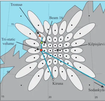
. The EISCAT radar measures the ion and electron tempera-tures, plasma density and line-of-sight ion velocity. The full ion velocity vector is determined within the tri-static volume. In the relatively collisionless regime of the F-region, the ions move with the E×B velocity, and hence the ion velocity measurements by EISCAT are representative of the electric field (e.g. Davies et al., 1999; Davies and Lester, 1999). Fig-ure 1 displays the location of the tri-static volume and the re-ceiver beam directions (in blue) in CP1-K mode of EISCAT. The red (green) circle represents the location of the tri-static (projected tri-static) volume at 278-km (110-km) altitude. As the electric field is approximately the same along the mag-netic field line, the tri-static volume was projected down to 110 km using the IGRF model. Figure 1 shows that in the E-and D-regions, it is the closest to the IRIS beam 16 E-and in this study the data from this beam were employed.
The International Monitor for Auroral Geomagnetic Ef-fects (IMAGE) Tromsø magnetometer measures local mag-netic perturbations in three perpendicular directions (L¨uhr et al., 1998). The position of the magnetometer is indicated by a red triangle in Fig. 1, which maps close to the pro-jected tri-static volume. The 20-s resolution data were post-integrated to give 1-min averages for this study. In order to obtain a Quiet Day Curve (QDC) for the magnetometer data, 2–4 days were chosen that were as close to each se-lected event as possible and that exhibited minimal perturba-tions. The dataset was then averaged for these quiet days and Fourier transformed. The number of harmonics was limited to 6 and then the inverse transform was taken to give the QDC for the event. The total horizontal magnetic perturbationsδH were obtained from components usingδH2=δX2+δY2.
The events in this study were selected based on the avail-ability of the tri-static ion drift velocity data from EISCAT.
15 25
70
Beam 16 Tromsø
20 69
Kilpisjarvi¨
Kiruna Tri-static
volume
Sodankyla¨
Fig. 1. Experimental setup diagram showing the IRIS and EISCAT
fields-of-view. The dots (ellipses) represent the intersection of the principal directions (−3 dB riometer beams) with the ionosphere at a height of 90 km. The−3 dB beams at the corners of the array are not shown as the antenna side lobes are too large. The 3 blue lines show the receiver beams from the EISCAT in the CP1-K common mode. The red circle shows the position of the tri-static volume at an altitude of 278 km. The green circle illustrates the position of the tri-static volume projected down the magnetic field line to 110 km in the E-region. At this height it is closest to beam 16 of the IRIS. The orange triangle is the position of the Tromsø magnetometer, which maps close to the projected tri-static volume.
The data from the CP1-K common mode for 46 days in 1995–1999 were analysed. An extended dataset compris-ing all available IRIS and IMAGE Tromsø data in Febru-ary 1995–JanuFebru-ary 1999 was also used in one part of this study (Sect. 3.3). All EISCAT velocity measurements above 2000 m/s and all IRIS absorption measurements below 0 dB were excluded. The effects of radio scintillations due to the passage of Cassiopeia over the IRIS field-of-view (FoV) were also removed from the IRIS data. The data from IRIS and IMAGE were then temporally matched with the EISCAT data to form a dataset comprised of simultaneous measure-ments.
Correlation: 0.47 Points: 14429 Max: 20
a
0 20 40 60 80 100 % Max
0 2 4 6 8
Velocity, 100 m/s 0.0
0.5 1.0 1.5 2.0 2.5 3.0
δ
H, 100 nT
b
Abs, dB
0.0 0.1 0.2 0.3 0.4 0.5
0 2 4 6 8 10
Velocity, 100 m/s
Correlation: 0.32 Points: 14373 Max: 20
c
0.0 0.1 0.2 0.3 0.4
IRIS Absorption, dB 0.0
0.5 1.0 1.5 2.0 2.5 3.0
δ
H, 100 nT
d
Vel, 100 m/s
0 2 4 6 8 10
0.0 0.1 0.2 0.3 0.4 0.5
IRIS Absorption, dB
Correlation: 0.02 Points: 14382 Max: 20
e
0 2 4 6 8
Velocity, 100 m/s 0.0
0.1 0.2 0.3 0.4 0.5
IRIS Absorption, dB
f
δH, 100 nT
0.0 0.6 1.2 1.8 2.4 3.0
0 2 4 6 8 10
Velocity, 100 m/s
Fig. 2. 2-D plots of(a, b)the IMAGE magnetic perturbationδH
versus the EISCAT ion velocity,(c, d)the IMAGE magnetic per-turbation versus the IRIS absorption, and(e, f)the IRIS absorption versus the EISCAT ion velocity for the entire dataset. In panels (a), (c) and (e) the occurrence of points for each cell up to a maximum of 20 is shown, colour-coded in percentage of maximum as indicated by the colour bar in panel (a). In panels (b), (d) and (f), the cells are colour-coded in the mean absorption, velocity, and perturbation, respectively, as shown on the right of each panel. The correlation for the entire dataset is shown in the top-left corner of panels (a), (c), and (e) along with the total number of points. The bin-averaged parameter dependence is shown by the white histogram.
(Hall or Pedersen) using a square root of squares technique (Brekke and Hall, 1988): 6Part2 =6Tot2 −6S2, where6Part and 6S are the particle and solar components of conductance,
respectively, and 6Tot is the total conductance. The solar component was calculated from the solar conductance model proposed by Robinson and Vondrak (1984).
3 Observations
3.1 Point-by-point comparisons and correlation analysis
In this section the relationships between magnetic perturba-tions, CNA, and the field-perpendicular component of the ion drift velocity are explored for both the entire dataset and for different MLT sectors. The data have been matched spatially and temporally, comprising of data points with three values representing the electrojet current strength, the Hall conduc-tance, and the ionospheric electric field, respectively. Two parameters are plotted against each other in a 2-D format while either the occurrence or the mean value for the third parameter is represented by the colour of the plot cell.
The comparisons over the entire dataset are displayed in Fig. 2. Panels (a, b) to (e, f) display the 2-D plots of perturba-tion versus velocity, perturbaperturba-tion versus absorpperturba-tion, and ab-sorption versus velocity, respectively. The left-column pan-els show the percentage occurrence of points for each cell, while the right-column panels are colour-coded in absorp-tion, velocity, and perturbaabsorp-tion, respectively, with the colour showing the averaged value over all measurements inside a given plot cell. The white histogram is the bin-averaged pa-rameter variation. The linear Pearson correlation co-efficient for the entire dataset is shown in the top-left corner of left-column panels along with the total number of points. The panels from (a, b) to (e, f) contain 91%, 83% and 81%, re-spectively, of the total points available after the previously defined restrictions were applied (Sect. 2).
Figure 2a shows an overall increase of perturbation with ion velocity, which is reflected in the overall positive corre-lation co-efficient of 0.47 and in the steady increase of the bin-averaged perturbation with ion velocity. There is some structuring in the corresponding panel (b) due to absorption variation which is evident in the colour coding. That is, the red and yellow cells tend to be in the top-left part of the di-agram with steady increase occurring in mean absorption as δHincreases and velocity decreases. This suggests that con-ductance also contributes to the electrojet current.
0.0 0.5 1.0 1.5 2.0 2.5 3.0
δ
H, 100 nT
0 - 3 MLT
Correlation : 0.38
Points : 2173 3 - 6 0.52
1827 6 - 9 0.27
1545 9 - 12 0.56 1875
0 2 4 6 8 10
Velocity, 100 m/s 0.0
0.5 1.0 1.5 2.0 2.5
δ
H, 100 nT
12 - 15 MLT
Correlation : 0.90 Points : 2323
2 4 6 8 10
Velocity, 100 m/s
15 - 18
0.72 2588
2 4 6 8 10
Velocity, 100 m/s
18 - 21
0.59 2260
2 4 6 8 10
Velocity, 100 m/s
21 - 0
0.28 2339
0.0 0.1 0.2 0.3 0.4 0.5 Abs, dB
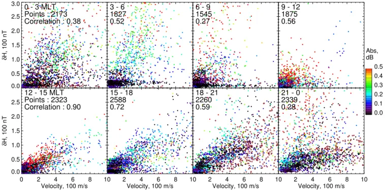
Fig. 3. Scatter plots of magnetic perturbation versus ion velocity for different MLT sectors. The correlation and total number of points are
also shown in the top-left corner of each panel. The colour coding is in absorption as shown to the right of the plot. The points with no simultaneous absorption measurements are shown by dark red pluses. The bin-averaged perturbation is shown by the red histogram.
as the correlation was higher in panel (b) and structuring was more pronounced in panel (d).
The comparisons between perturbation and ion velocity (absorption) have demonstrated positive correlation and ob-vious structuring in Fig. 2b (Fig. 2d). In panels (e, f) ab-sorption and velocity are compared directly with the colour coding in panel (f) in the IMAGE magnetic perturbation. This comparison reveals no significant correlation or anti-correlation between these parameters for the entire dataset. Data does seem, however, to be spread along the both axes in panel (f) suggesting a possible inverse proportionality re-lationship, which is also evident in the 2-D occurrence plot of panel (e). This is emphasized in panel (f) by structuring of the cells according to colour with blue (red) cells gener-ally closer to (farther from) the axes. Red cells (large mean perturbations) are observed in the top-right quadrant of the diagram where both absorption and velocity are large.
Although some correlation was found when analysing the three parameters over the entire dataset, the temporal vari-ation of this correlvari-ation was not investigated. In the latter part of this section we investigate the time variation of these correlations in three-hour MLT blocks (MLT=UT+2.7). This should give an indication of how the conductance and electric field control of electric current varies with MLT.
In Fig. 3 the data have been divided into 8 three-hour time sectors by MLT. For each time sector the perturbation is plot-ted against the ion drift velocity. The correlation is shown, along with the number of points in the top-left corner of each panel. The colour coding is in absorption and is the same
for all time sectors as displayed on the right of the figure. The dark red pluses represent points without colour coding information that were nevertheless included in the correla-tion analysis. The figure shows that the correlacorrela-tion is high-est just after magnetic noon (0.90 at 12:00-15:00 MLT) and stays quite high until 21:00 MLT where it sharply decreases to 0.28. It is minimised in the midnight sector before ris-ing again in the mornris-ing sector (03:00-06:00 MLT). The two features of interest in the figure are the rapid increase in cor-relation at 12:00 MLT and the sharp decrease at 21:00 MLT with the colour coding in absorption also showing some in-teresting results. There is more data structuring near mid-night (where red points are at the top and black points are at the bottom) and less in the afternoon, possibly indicating a higher correlation between absorption and perturbation near midnight and less correlation near noon, which is explored next.
0.0 0.5 1.0 1.5 2.0 2.5 3.0
δ
H, 100 nT
0 - 3 MLT
Correlation : 0.76
Points : 1479 3 - 6 0.65
1348 6 - 9 0.50
1016 9 - 12 0.08 1254
0.0 0.1 0.2 0.3 0.4 0.5
IRIS Absorption, dB 0.0
0.5 1.0 1.5 2.0 2.5
δ
H, 100 nT
12 - 15 MLT
Correlation : 0.17 Points : 1580
0.1 0.2 0.3 0.4 0.5
IRIS Absorption, dB
15 - 18
0.09 1912
0.1 0.2 0.3 0.4 0.5
IRIS Absorption, dB
18 - 21
0.30 1267
0.1 0.2 0.3 0.4 0.5
IRIS Absorption, dB
21 - 0
0.69 1549
0 2 4 6 8 10 Vel, 100 m/s
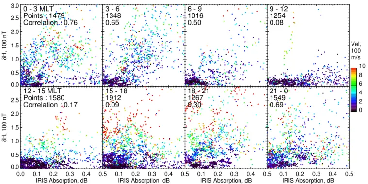
Fig. 4. The same as Fig. 3 except magnetic perturbation and absorption are compared and colour-coded in velocity.
0.0 0.5 1.0 1.5 2.0
IRIS Absorption, dB
0 - 3 MLT
Correlation : 0.30
Points : 1573 3 - 6 0.30
1473 6 - 9 0.08
1163 9 - 12 0.00 1385
0 2 4 6 8 10
Velocity, 100 m/s 0.0
0.5 1.0 1.5
IRIS Absorption, dB
12 - 15 MLT
Correlation : 0.04 Points : 1706
2 4 6 8 10
Velocity, 100 m/s
15 - 18
0.12 2071
2 4 6 8 10
Velocity, 100 m/s
18 - 21
0.13 1373
2 4 6 8 10
Velocity, 100 m/s
21 - 0
0.21 1652
0.0 0.6 1.2 1.8 2.4 3.0
δH,
100 nT
Fig. 5. Same as Fig. 3 except absorption and velocity are compared and colour-coded in perturbation.
To complete the analysis, the relationship between absorp-tion and ion velocity is examined in Fig. 5, where points are now colour-coded in perturbation. The correlation is highest in the post-midnight/early-morning sector 00:00–06:00 MLT (0.30) and very low for the other time sectors. There is,
0.27 0.56 0.90 0.72 0.59 0.28 0.38 0.52 0.50 0.08 0.17 0.09 0.30 0.69 0.76 0.65 06 09 12 15 18 21 00 Magnetic Local Time
03 ρ(δH,Ui) ρ(δH,A) (a) 0.74 0.17 0.19 0.25 0.49 0.73 0.77 0.69 0.73 0.09 0.20 0.37 0.49 0.70 0.76 0.64 06 09 12 15 18 21 00 Magnetic Local Time
03
ρ(δH,ΣH Tot) ρ(δH,ΣH Part)
(b)
Fig. 6. Clock diagrams showing the correlation of magnetic
pertur-bation(a)with ion velocity (absorption) in blue (red) and(b)with the total (particle component) Hall conductance in outer (inner) cir-cular band for different MLT. The colour coding is representative of the correlation from low (dark) to high (light).
3.2 Correlation clock diagrams
The results of the correlation analysis presented above are summarised in Fig. 6a which presents the level of correla-tion for each 3-h time sector both numerically and by the colour of the sector with lighter (darker) shades representing a higher (lower) correlation. The correlation co-efficients be-tween magnetic perturbations and ion velocity (absorption) ρ(δH, Ui)[ρ(δH, A)] are indicated in blue (red) colour in
the outer (inner) circle. Figure 6a suggests that, overall, the electric field exerted more dominance over the electrojet cur-rents than the conductance. Thus both the overall and maxi-mum correlations are higher forρ(δH, Ui)thanρ(δH, A):
0.47 and 0.90 versus 0.32 and 0.76. Also, roughly com-plementary trends/relationships are observed in Fig. 6a, i.e. the current-velocity correlation is substantial whenever the current-absorption correlation is low and vice versa.
We have also performed a similar correlation analysis with the actual Hall conductance rather than with its proxy. The magnetic perturbation correlations with the total (with so-lar contribution) and particle component of Hall conduc-tance were determined for each 3-h MLT sector. The re-sults are presented in Fig. 6b. All three types of correla-tion shown in red in Fig. 6 show a very similar picture. Re-calling that CNA is not representative of the Hall conduc-tance at 15:00–19:00 MLT (Senior et al., 2007), we observe that the ρ(δH, A) and ρ(δH, 6Part) correlations exhibit a generally good agreement outside of the 15:00–21:00 MLT sector. The ρ(δH, 6Tot) and ρ(δH, 6Part) are also quite close with the differences most pronounced on the day-side, in particular at 09:00–12:00 and 15:00–18:00 MLT. The only observation inconsistent with our simple paradigm suggesting that absorption is a good proxy for particle component of conductance is at 06:00–09:00 MLT when ρ(δH, A)<ρ(δH, 6Part)∼=ρ(δH, 6Tot), which may be due to a failure of the solar conductivity model to fully remove solar effects for this particular subset of data.
06 09 12 15 18 21 00 03 Vernal 1995 1996 1997 1998 All years
(a)
06 09 12 15 18 21 00 03 Summer(b)
06 09 12 15 18 21 00 Magnetic Local Time03 Autumnal
(c)
06 09 12 15 18 21 00 Magnetic Local Time03 Winter 0.0 0.2 0.4 0.6 0.8 1.0 Correlation
(d)
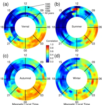
Fig. 7. Clock diagrams showing the correlation co-efficients
be-tween magnetic perturbations and absorption for 1-h boxcar cor-relations calculated at 1-min resolution for different seasons. The colour coding is representative of the correlation as indicated by the colour bar. The circular bands in each panel represent different years as indicated at the top of the diagram.
3.3 Auroral absorption and currents for different seasons
In our previous analysis, the dataset was limited to 46 days with simultaneous EISCAT ion velocity data. Our novel ap-proach involving simultaneous and coincident magnetometer and riometer measurements provides a unique opportunity to explore in more detail the statistical current-conductance relationship (using CNA as a proxy). In this section, we employ an extended Tromsø magnetometer/IRIS riometer dataset collected over the 4 years February 1995–January 1999. This period is selected to include 81 days around equinoxes and solstices, that is why 4 calendar years 1995– 1998 are shifted by 1 month. Both datasets have 1-min time resolution so that up to 1440 data points are available for each day. The large amount of data also allowed us to im-prove drastically the time resolution of the correlation analy-sis. This has been done by calculating the boxcar correlation co-efficients for a 1-h period centered on every minute. The boxcar correlation dataset thus comprised 1440 values (for each min) with each of them calculated using up to 60Nd
points, whereNd is the number of days in a considered
pe-riod.
-0.2 0.0 0.2 0.4 0.6 0.8
ρ
(
δ
H, U
i
)
Mean
Median
a
-0.2 0.0 0.2 0.4 0.6 0.8
ρ
(
δ
H, A)
b
0 5 10 15 20
Time, MLT -0.2
0.0 0.2 0.4 0.6 0.8
ρ
(A, U
i
)
c
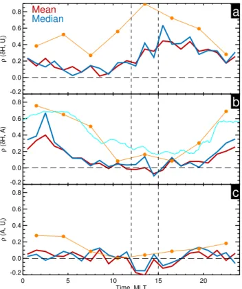
Fig. 8. Line plots of the hourly correlation co-efficients between
(a)perturbation and velocity,(b)perturbation and absorption, and (c)absorption and velocity. The red (dark blue) line represents the mean (median) value of the hourly correlation co-efficients. The orange dots and lines represent the 3-hourly correlation coefficients from Figs. 3–5. In panel (b) the light blue line shows a 1-h boxcar correlation computed using an extended dataset.
spring, summer, autumnal and winter periods, respectively. In addition, the data has been further restricted to specific years as shown by different circular bands (Nd=81). The
year specified for each circular band in panel (a) is that at the start of each 81-day period. The correlation co-efficients for all years combined are also shown in the innermost circular band (Nd=324). The correlation is represented by the colour
as shown by the colour bar in the centre of the plot.
Figure 7 shows a lot more detail in correlation as a func-tion of MLT than Fig. 6. For majority of the years, the re-gion of high correlation extends from 21:00 to 06:00 MLT during the equinoctial periods, panels (a) and (c), which is also reflected in all-years correlations. During the summer period, panel (b), it is shifted later into the morning and cov-ers a smaller MLT range (02:00–07:00 MLT). There is also an “anomalous” region of very high correlation near local noon for summer 1996. The winter period, panel (d), dis-plays highly variable correlation with no clearly defined re-gion of high correlation consistent over the years. The cor-relation on the dayside before 12:00 MLT, however, is no-ticeably higher than in other seasons. One can conclude that
the current-absorption correlation exhibits a distinct seasonal dependence. One should bear in mind though that the corre-lation values at 15:00–19:00 MLT are not representative of the current-conductance correlation (Senior et al., 2007). 3.4 Hourly correlation analysis
Figures 3–5 summarised in Fig. 6a revealed that the correla-tion between the 3 parameters varied throughout the day. The correlation co-efficients were calculated for each 3-h sector. In Sect. 3.3 the correlation co-efficients were also computed using 1-h boxcar periods. In both analyses the correlations were calculated for all events combined together. In this sec-tion the correlasec-tion is further examined using a different anal-ysis. The correlation co-efficients are calculated at hourly in-tervals for each event and then averaged over the 46 events for each hourly period in MLT. We will refer to these val-ues as “hourly” correlations to distinguish from “1-h” box-car correlations from Sect. 3.3 and “3-h” correlations from Sects. 3.1–3.2. A similar hourly correlation analysis was em-ployed earlier by Makarevitch and Honary (2005).
The correlation co-efficient for each hourly period was only calculated and entered into the dataset if there were suf-ficient number of points in the hourly period. This was de-termined by comparing the data available for each hour to the maximum number of data points that the instrument was capable of collecting during the hour (typically 30 points for EISCAT and 60 points for IRIS and IMAGE). If this number was greater than 60% then the number of points was deemed sufficient.
In order to compare the results from the hourly correlation analysis with those presented in Figs. 3–6, the mean and me-dian hourly correlation co-efficients were calculated over the entire dataset for each of the 3 pairs of parameters. These are presented as a function of MLT in Fig. 8. The 3-h values from Figs. 3–5 are also shown for reference by the orange lines. The extended IMAGE/IRIS dataset of Sect. 3.3 was em-ployed in panel (b) to compute 1-h boxcar correlations (light blue) over the entire 4-year dataset (Nd=365.25×4=1461).
The 1-h boxcar correlations for the extended dataset show very similar variation to 3-h values. Panel (a) clearly shows the hourly correlationρ(δH, Ui)starting low in the midnight
to early morning sector, then rising quickly after 12:00 MLT and reaching a maximum just after the 12:00–15:00 MLT sector. It then drops off more smoothly through the after-noon. An almost opposite pattern is observed between per-turbation and absorptionρ(δH, A)in panel (b). The correla-tion is highest just post-midnight between 02:00–03:00 MLT and smoothly drops off to reach a minimum during the 12:00–15:00 MLT sector. It then rises again to higher values pre-midnight. Panel (c) displays a low correlationρ(A, Ui)
3-h correlations. The hourly correlations are smaller than ei-ther 3-h or 1-h boxcar values, which is most likely indicative of some over-averaging occurring in this approach.
3.5 Electron heating absorption
The two analyses presented in the previous sections (Figs. 3 and 8) revealed that the data from the afternoon sector exhib-ited enhanced correlation between magnetic perturbation and ion velocity. This suggested that the electric field is a pre-dominant factor in determining the electrojet current strength in the afternoon. One can argue that the correlation between conductance and electric fields should be maximised during the periods when the correlation between perturbation and ion velocity is close to 1. In this situation, the electric field affects the current both directly (as current is proportional to the electric fieldJ∝E) and indirectly through conductance, collision frequency, and temperature (J∝6∝νe∝Te1/2) with
the latter increasing with electric field. This should result in the maximum correlation observed. To test this idea, 9 days exhibiting high hourly correlations between perturbation and ion velocity were extracted from the dataset. On average, the period of maximum correlation for each interval was found to be close to the high correlation period of 12:00-15:00 MLT in Fig. 3 and this 3-h period was selected as the common period for all 9 days. The days selected, in “yyyymmdd” format, were: 19950301, 19950302, 19950329, 19950928, 19960214, 19960619, 19961211, 19970515 and 19990212.
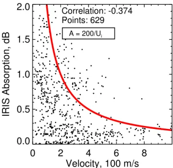
Figure 9 displays a comparison between absorption and ion velocity for the high correlation period days. The dia-gram format is the same as for each panel in Fig. 5. However, in Fig. 9 the dataset is restricted to the 12:00–15:00 MLT sec-tor for the 9 selected days. An inverse proportionality is apparent in the data, similar to that observed in the 09:00-15:00 MLT sectors in Fig. 5. The red line represents a curve of inverse proportionality defined byA=200/Ui, whereAis
the IRIS absorption andUi is magnitude of the EISCAT ion
drift velocity. The choice of a constant in this simple model is rather arbitrary; for this study a value of 200 dB/m/s was selected to best represent the structuring of the data, in par-ticular that the upper envelope of the data points follows the inverse proportionality curve. As will be argued later, this feature is consistent with the notion of limiting of the current by the magnetospheric generator. No significant correlation between the ion velocity and absorption is found in this ap-proach though.
The electron heating effects are expected to exhibit a threshold in the ion drift velocity as the two-stream instability (which is responsible for electron heating) is only operational when the drift velocity exceeds the ion acoustic speed. The accepted value for the threshold velocity is∼400 m/s (e.g. Fejer and Kelley, 1980, and references therein). However, Fig. 9 showed little evidence of absorption increase with the ion drift velocity (expected in the EHA mechanism) either at small or at large, above-the-threshold ion velocities.
0
2
4
6
8
Velocity, 100 m/s
0.0
0.5
1.0
1.5
2.0
IRIS Absorption, dB
Correlation: -0.374
Points: 629
A = 200/Ui
Fig. 9. Scatter plot of absorption versus velocity for the 12:00–
15:00 MLT time sector for 9 days exhibiting high correlation inter-vals within this period (see text for details). The format is the same as for each panel in Fig. 5. The red curve represents an inverse proportionality trend described by the equation shown on the graph.
Another approach is to consider the absorption depen-dence on the electron temperatureTe as this is expected to
show a more direct effect on absorption through collision frequency:A∝νe∝Te1/2. The electron temperature in the
E-region centre, in turn, is expected to show some dependence on the drift velocity above the velocity threshold (e.g. Davies and Robinson, 1997). Consequently, in the following analy-sis only theTe data points at a height of 111 km and above
the certain temperature threshold were considered. Simi-lar to Davies and Robinson (1997), the electron temperature data were obtained using the alternating code technique. The electron and ion temperatures were derived from the separa-tion and sharpness of the two peaks in the ion acoustic spec-tra measured by EISCAT; no equality between them was as-sumed (Rishbeth and Williams, 1985).
The threshold values for temperature were determined for different 3-h MLT sectors as follows. The electron temper-atures were plotted versus the ion drift velocity (not shown here). These plots showed a quadratic-like temperature in-crease with velocity but with different rates of inin-crease for different MLT. This result was reminiscent of the similar quadratic dependence found to well represent the ion acous-tic speedCs=A+BUi2with fitting co-efficientsAandB
de-pendent on MLT (e.g. Nielsen and Schlegel, 1985; Makare-vich et al., 2007). In this study, we used a similar approach, in which a quadratic function of the formTe=C+DUi2was
fitted to the data for each MLT sector. The threshold elec-tron temperature T∗
2
4
6
8
10
T
e, 100 K
0.0
0.5
1.0
1.5
2.0
IRIS Absorption, dB
0
4
8
12
16
20
24
MLT
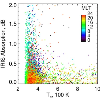
Fig. 10. Scatter plot of absorption versus the electron temperature
colour-coded in MLT. The data in each MLT sector is restricted to include temperatures above the threshold electron temperature (see text for details).
substituting U∗
i =400 m/s into the above equation. Above
T∗
e, the electron temperature should be affected by the
heat-ing associated with the unstable two-stream waves (see our Sect. 1). Thus one can further explore the electron heating effects by restricting the absorption versus electron tempera-ture data to above-the-threshold values.
The results of this analysis are displayed in Fig. 10 which shows absorption versus the electron temperature colour-coded in MLT. Figure 10 shows that, overall, there appears to be no direct relationship between the two parameters ei-ther near the threshold (300–400 K) or well above it (e.g. >600 K). Interestingly, a possible inverse proportionality re-lationship can be recognized, similar to that in Fig. 9. One can conclude thus that little evidence of electron heating ab-sorption was observed in this study.
4 Discussion
In this paper, the magnetic perturbations, ion velocity, and absorption were compared and the relationship between the current, electric field, and conductance in the auroral region was studied. Compared to previous studies, the MLT cov-erage was extended to all time sectors including the day-side and the height-integrated characteristic of absorption was used as a proxy for the ionospheric conductance in-stead of the conductance estimates from incoherent radars. Also, most of the previous statistical studies have drawn their conclusions from analysis and comparison of the aver-aged/median MLT variations of the electric fields, currents,
and conductances. In this study, we used a somewhat dif-ferent approach in which the measurements were compared and correlated within each MLT sector, Sects. 3.1–3.2. We also employed a significantly larger dataset of simultaneous magnetometer/riometer observations collected over 4 years to statistically investigate the current-absorption relationship in Sect. 3.3. This approach was complemented by the hourly correlation analysis of Sect. 3.4.
4.1 Electric field and conductance control of currents
An important thing to bear in mind while interpreting the re-sults of the current study is that riometer measurements pro-vide information on the particle component of conductance. One can expect that on the dayside the correlation between the current intensity and total conductance (due to both solar radiation and precipitation) would be larger. Figure 6b sup-ports this assumption with most time sectors showing larger correlation with the total conductance. The fact that in one time sector (15:00–18:00 MLT) the correlation was signifi-cantly smaller (0.25 vs. 0.37) suggests that this simple view is not necessarily always correct.
From above, one should be careful when drawing con-clusions in relation to the relative importance of electric field and conductance based on the ρ(δH, A) correlation only. However, it is reasonable to expect that the solar con-tribution would not change the correlation so significantly so that it will exceed theρ(δH, Ui)correlation in the
sec-tors whereρ(δH, A) is low andρ(δH, Ui)is high, i.e. at
09:00–21:00 MLT. Again, this is strongly supported by Fig. 6 that shows that the enhanced correlation due to inclusion of the solar conductanceρ(δH, 6Tot)still does not exceed ρ(δH, Ui). By the same token, ifρ(δH, A)is substantially
greater thanρ(δH, Ui)(at 21:00–09;00 MLT) and hence the
particle component conductivity dominates over the electric field, this is likely to be the case for the total conductance as well, which agrees well with Fig. 6.
Another possible complication is that magnetometers pro-vide information on the Hall current rather than the to-tal (Hall and Pedersen) current. However, as absorption is closely related to the Hall conductance, the comparisons performed in this study involve the three parameters that are expected to be related via a simple proportionality rule: JH=6HUiB. One has to nevertheless bear in mind that
in-terpreting the observations in terms of the total current may not be so simple in some cases. One important case though when this is possible is when the Hall and Pedersen currents vary synchronously, which happens when they are both con-trolled by the electric field. That is, one can assume that high ρ(δH, Ui)values imply high total-current-electric-field
by other researchers (e.g. Kamide and Vickrey, 1983), so that comparisons with their results will provide a straightforward way of verifying our results and conclusions.
Kamide and Vickrey (1983) and Davies and Lester (1999) demonstrated that on the nightside throughout the eastward convection electrojet the electric field is the dominant fac-tor and that the Hall conductance tends to dominate in the westward electrojet. So the transition from the eastward to westward electrojets is commonly believed to coincide with a transition from electric-field- to conductance-driven currents. In our observations, the transition between MLT sectors with high and lowρ(δH, Ui)occurred at 21:00 MLT in Fig. 6a,
which is consistent with pre-midnight location of transition from the eastward to westward electrojets.
Interestingly, ρ(δH, Ui) values temporarily increased
again at 03:00–06:00 MLT. This feature may be related to the transition between the conductivity- and electric-field-dominant regions reported by Kamide and Vickrey (1983) to occur in the late morning (near 03:00 MLT) within the west-ward electrojet. Extending the same argument further to-wards the dayside, one can propose that a drop inρ(δH, Ui)
at 06:00–09:00 MLT is due to relative weakening of the elec-tric field control in this time sector. Statistically, Sugino et al. (2002) showed that for all Kp conditions the electric field
orientation switched from southward to northward in the late morning sector, just prior to 12:00 MLT, which is normally a characteristic of a change from the westward to eastward convection electrojets. The substantial increase inρ(δH, Ui)
across the 12:00 MLT boundary and considerableρ(δH, Ui)
correlations at 09:00–21:00 MLT observed in this study thus suggest that the entire eastward convection electrojet is dom-inated by the electric field including the dayside.
This is contrary to the situation in the westward electro-jet that exhibited consistently large values ofρ(δH, A) al-though variable ρ(δH, Ui) correlations. The former
fea-ture suggests that the westward electrojet is predominantly conductivity-driven. This result disagrees somewhat with that by Kamide and Vickrey (1983) who demonstrated that the westward electrojet in the late morning sector is electric-field-dominant. However, this result is consistent with the statistical study by Davies and Lester (1999) who also did not observe the opposite transition within the westward elec-trojet. An increase inρ(δH, Ui)observed in our study at
03:00–06:00 MLT was reminiscent of this opposite transi-tion, however theρ(δH, A)value was still quite substantial (0.65) so that, overall, it is difficult to conclude whether the electric-field-dominant region is observed within the west-ward electrojet on a statistical basis using the EISCAT-restricted events. One possible reason is that this feature may only be seen during substorm intervals. However, the results of Fig. 7 based on the extended dataset showed that conductivity-dominant region is 21:00–06:00 MLT near the equinoxes and only 02:00–07:00 MLT in summer. Thus the statistical behaviour near the equinoxes is in agreement with Kamide and Vickrey (1983).
An extension of the conductivity-driven region into the late morning up to 09:00 MLT suggested by the present study is also in rough agreement with the conductivity-dominant interval of 20:00–08:00 MLT proposed by Sugino et al. (2002). These authors observed two peaks of con-ductivity dominance: one near midnight and one in the late morning around 06:00 MLT. This result also agrees well with our observations that showed a significant drop inρ(δH, Ui)
at 06:00–09:00 MLT. One should note that the positive dif-ference between ρ(δH, A) and ρ(δH, Ui) in the 06:00–
09:00 MLT sector becomes even larger if solar contribu-tion to conductance is taken into account, Fig. 6b, so that the above conclusion that the entire westward electrojet is conductivity-dominant is not affected.
Figure 6a also shows that highρ(δH, A)correlation starts abruptly at 21:00 MLT, continues through the midnight sec-tor, and stretches out into the morning sector where it slowly declines. We believe that this slow decline may be attributed to the slowly varying absorption (SVA) effect (Stauning, 1996a) as described below. The energetic particle precipi-tation could easily ionise particles in the upper D- to lower E-regions to which the Hall conductivity and CNA are most sensitive. Satellite observations employed by Collis et al. (1984) showed that the spectrum of drifting electrons hard-ens with increasing time up to 09:00 MLT, which for the same particle flux would cause a larger detected CNA and correlation with the Hall current. The sharp fall inρ(δH, A) across the 09:00 MLT border is consistent with this idea. The steady decrease in correlation through the morning sector to 09:00 MLT seems to be inconsistent with Collis et al. (1984), as one would expect the correlation to increase with the hard-ening electron spectrum. However, the decline in correlation with increasing MLT may be related to the eventual deple-tion of the electron clouds drifting around the Earth east-ward toeast-wards the dayside. This results in more energetic but less intense precipitation, which would contribute less to the conductance. Local substorms are also more likely to occur at 19:00–04:00 MLT, which would enhance the conductance and hence the current together with the CNA detected by the IRIS at these times. Substorms thus may account, in part, for the larger correlation observed at earlier MLT.
number flux on the dayside and a corresponding increase in energy flux in summer as compared to winter reported by Liou et al. (2001) (see their plates 3–5), while the first obser-vation appears not to have a direct counterpart in low-energy (<10 keV) particle observations. This suggests that absorp-tion signatures of the high-energy particles, in particular in the context of their relationship with auroral currents, are sig-nificantly different from their low-energy counterparts.
Our observations suggest that, on average, the conductance- (electric-field-) dominant region is centered at 00:00–03:00 (12:00–15:00) MLT. This result is consistent with previous statistical studies that found that the west-ward electrojet centre was generally located post-midnight (Kamide, 1991). The post-midnight shift was explained by the DP2 (DP1) current system contributing to the westward electrojet at 00:00–06:00 MLT (21:00–03:00 MLT) so that averaging over all events shifts the westward electrojet center, and hence the conductivity-dominant region centre, from midnight to the early morning.
In Fig. 6a, a similar shift (towards later MLT) is also ob-served in the current-velocity correlation which is substan-tial at 09:00–21:00 MLT. This overall rotation of the electric-field-dominant region clockwise from the noon-midnight meridian could be related to the properties of the plasma con-vection pattern as discussed below. The high-latitude plasma convection pattern is known to depend strongly on the direc-tion and magnitude of the IMFBy component (e.g. Heelis,
1984). Statistically, Ruohoniemi and Greenwald (2005) and, more recently, Haaland et al. (2007) demonstrated the lack of mirror-symmetry between the effects of positive and neg-ative IMFBy. Similar results for several events during small
By conditions were also reported by Kustov et al. (1998).
The significant shift towards earlier MLT in location of the “throat” region (where plasma flows into the polar cap) and the resulting rotation in the convection cells only occurred for positive (negative) IMFByin the Northern (Southern)
Hemi-sphere (Haaland et al., 2007). This implies that, on average, the transition between the westward to eastward convection electrojet occurs in the late morning sector. The results of the current study are consistent with these findings, as in our observations the transition from the conductance- to electric-field-dominant region also occurred in the late morning, at 09:00 MLT in Fig. 6a.
4.2 Auroral absorption and electric field
In Figs. 2e and 2f absorption was compared with the ion velocity over the entire dataset and a negligible correla-tion found. Although one expects no direct relationship between absorption (conductance) and plasma convection speed (electric field), various indirect links have been pro-posed in the past including the electron heating mechanism in which absorption may exhibit an increase with the electric field (see Sect. 1). No such increase was seen in Figs. 2e, 2f, 5, 9. Thus these results indicate that no evidence of electron
heating absorption is observed on a statistical basis in the au-roral zone. However, an interesting result was that in Fig. 8c some anticorrelation was observed at 12:00–15:00 MLT and that in Figs. 5 (09:00–15:00 MLT) and 9, an inverse propor-tionality was present.
The inverse proportionality between absorption and plasma velocity found in this study can be explained if a simple model of the magnetospheric generator is used such as that proposed by Robinson (1984), based on the work done by Reiff et al. (1981). In the magnetospheric gener-ator model, the field-aligned currents are assumed to flow in large sheets that are connected in the ionosphere by Ped-ersen currents. The field-aligned current integrated across one sheet, J0, is fixed, but the magnetospheric convection and the electric field adjust themselves to ionospheric con-ductance variations. Therefore the Pedersen currents, which close the circuit in the ionosphere, are limited byJ0, so that 6PE=JP≤J0. The observed inverse proportionality
rela-tionship between the conductance and electric field can thus be attributed to this limit on the Pedersen current. If the cur-rent is limited then any further increase in the electric field must be associated with a decrease in the Pedersen conduc-tance and vice versa. Later this limitation was described in terms of the magnetospheric current generator (or source) as opposed to the voltage generator in which the electric field does not change much regardless of conductance changes (Fujii and Iijima, 1987).
There are two potential problems with this interpretation though. Firstly, the simple magnetospheric generator model suggested by Robinson (1984) would not hold in perturbed current systems such as that observed in the midnight sec-tor when precipitation is the main contribusec-tor to currents and DP1 systems are in action. Secondly, the magnetic pertur-bations are mostly representative of the Hall currents, while CNA correlates best with the Hall conductance (Senior et al., 2007). However, the time period 12:00–15:00 MLT is away from the midnight sector and provided that the Pedersen and Hall currents varied more or less synchronously, the sim-ple model of Robinson (1984) can be employed as a pos-sible explanation of our results. As mentioned, one can cer-tainly expect the two currents to vary synchronously during the high correlation periods between the current and elec-tric field. The data collected in the 09:00–12:00 and 12:00– 15:00 MLT sectors in Fig. 5 for the entire dataset also showed some evidence of inverse proportionality, which suggests that the especially high correlation between electric fields and the current may not be necessary. Rather, an electric field control during the late morning and early afternoon in general, could be indicative of the magnetospheric generator effect.
or well above it in any MLT sector. However, a possible in-verse proportionality relationship could be seen in the data, which was reminiscent of the relationship between the ab-sorption and the electric field.
5 Summary and conclusions
The relationship between magnetic perturbations, absorp-tion, and ion drift velocity was studied, for the first time, using a temporal correlation analysis technique for differ-ent MLT sectors. This analysis method was augmented by an hourly correlation analysis for individual events which displayed a similar MLT variation of mean and me-dian hourly correlations. In addition, an extended per-turbation/absorption dataset was considered with correla-tions showing a distinct seasonal dependence. This study demonstrates the strong potential of riometers in studies of the current-conductance-E-field relationship, particularly in combination with magnetometers.
The current-electric-field correlation was generally higher than the current-absorption correlation, which suggests that, on average, the electric field is more dominant in the control of the current than conductance. The current-electric-field correlation was found to be higher on the dayside (09:00– 21:00 MLT). It was maximised in the 12:00–15:00 MLT sec-tor reaching 0.90, with a sharp increase across the 12:00 MLT border. The current-absorption correlation was higher on the nightside (21:00–09;00 MLT) reaching its maximum of 0.76 in the post-midnight sector (00:00–03:00 MLT). This sug-gests that the conductance is more dominant on the nightside. The transition from an electric-field-dominant region to a conductivity-dominant region in the pre-midnight sector (21:00 MLT) was associated in the past with a transition from eastward to westward electrojet currents. The results from the nightside showing predominantly conductivity-driven current were generally consistent with previous sta-tistical studies, with some evidence of the opposite transition observed in the late morning sector near 03:00 MLT, which was previously observed only for individual events. An ex-tension of the conductivity-dominant region to 09:00 MLT with a gradual decrease in the current-absorption correla-tion was also observed, which was explained as being in part due to energetic electrons drifting eastward around the Earth and gradually precipitating in the morning sector. The analysis of the extended 4-year dataset discovered a dis-tinct seasonal dependence in the absorption-current rela-tionship. The region of high current-absorption correlation was found to be at 21:00–06:00 MLT near the equinoxes, while in summer it was narrower and rotated towards dawn 02:00–07:00 MLT. The significant asymmetry/rotation of the electric-field-dominant region with respect to the 00:00– 12:00 MLT meridian found in this study, may be related to the lack of mirror symmetry between the effects of positive and negative IMFByon the plasma convection pattern.
There was no correlation found between absorption and electric field for the entire dataset. Also, no significant cor-relation was found for different MLT sectors, during peri-ods of high correlation between electric fields and current, or for drift velocities and electron temperatures above the two-stream instability threshold. Thus no substantial evidence of electron heating absorption in the auroral zone was found. However, an inverse proportionality was found between the absorption and electric field during the high current-E-field correlation periods and, generally, in the 09:00–15:00 MLT sector, which was attributed to a limit on the Pedersen cur-rent imposed by the magnetospheric generator during these time intervals.
Acknowledgements. This research was supported by the
Aus-tralian Research Council Discovery grant to R. A. M. (project DP0770366). The Imaging Riometer for Ionospheric Studies (IRIS) is operated by the Department of Communications Systems at Lan-caster University (UK) in collaboration with the Sodankyl¨a Geo-physical Observatory, and funded by the Science and Technology Facilities Council (STFC). The IMAGE magnetometer data are collected as a Finnish-German-Norwegian-Polish-Russian-Swedish project conducted by the Technical University of Braunschweig and Finnish Meteorological Institute. EISCAT is an International Association supported by Finland (SA), France (CNRS), Germany (MPG), Japan (NIPR), Norway (NFR), Sweden (NFR), and the UK (STFC). The authors thank H. Yamagishi, A. Grocott, and Y. Bog-danova for useful discussions and suggestions.
Topical Editor M. Pinnock thanks S. Buchert and another anony-mous referee for their help in evaluating this paper.
References
Amm, O.: The elementary current method for calculating iono-spheric current systems from multi-satellite and ground magne-tometer data, J. Geophys. Res., 106, 24843–24855, 2001. Brekke, A. and Hall, C.: Auroral ionospheric quiet summer time
conductances, Ann. Geophys., 6, 361–375, 1988, http://www.ann-geophys.net/6/361/1988/.
Browne, S., Hargreaves, J. K., and Honary, B.: An imaging riometer for ionospheric studies, Electronics and Communication, 7, 209– 217, 1995.
Collis, P. N., Hargreaves, J. K., and Korth, A.: Auroral radio ab-sorption as an indicator of magnetospheric electrons and of con-ditions in the disturbed auroral D-region, J. Atmos. Terr. Phys., 46, 21–38, 1984.
Davies, J. A. and Lester, M.: The relationship between electric fields, conductances and currents in the high-latitude ionosphere: a statistical study using EISCAT data, Ann. Geophys., 17, 43–52, 1999, http://www.ann-geophys.net/17/43/1999/.
Davies, J. A. and Robinson, T. R.: Heating of the high-latitude iono-spheric plasma by electric fields, Adv. Space Res., 20, 1125– 1128, 1997.
Fejer, B. G. and Kelley, M. C.: Ionospheric irregularities, Geophys. Rev., 18, 401–454, 1980.
Fujii, R. and Iijima, T.: Control of the ionospheric conductivities on large-scale Birkeland current intensities under geomagnetic quiet conditions, J. Geophys. Res., 92, 4505–4513, 1987.
Haaland, S. E., Paschmann, G., F¨orster, M., Quinn, J. M., Torbert, R. B., McIlwain, C. E., Vaith, H., Puhl-Quinn, P. A., and Klet-zing, C. A.: High-latitude plasma convection from Cluster EDI measurements: method and IMF-dependence, Ann. Geophys., 25, 239–253, 2007,
http://www.ann-geophys.net/25/239/2007/.
Heelis, R. A.: The effects of interplanetary magnetic field orienta-tion on dayside high-latitude ionospheric convecorienta-tion, J. Geophys. Res., 89, 2873–2880, 1984.
Kamide, Y.: The auroral electrojets: Relative importance of iono-spheric conductivities and electic fields, pp. 385–399, in: Auroral Physics, edited by: Meng, C.-I., Rycroft, M. J., and Frank, L. A., Cambridge University Press, Cambridge, 1991.
Kamide, Y. and Vickrey, J. F.: Relative contribution of ionospheric conductivity and electric field to the auroral electrojets, J. Geo-phys. Res., 88, 7989–7996, 1983.
Kustov, A. V., Lyatsky, W. B., and Sofko, G. J.: Super Dual Auroral Radar Network observations of near-noon plasma convection at small interplanetary magnetic field Bz and By, J. Geophys. Res., 104, 4041–4050, 1998.
Liou, K., Newell, P. T., and Meng, C.-I.: Seasonal effects on auro-ral particle acceleration and precipitation, J. Geophys. Res., 106, 5531–5542, 2001.
L¨uhr, H., Aylward, A., Bucher, S. C., Pajunp¨a¨a, A., Pajunp¨a¨a, K., Holmboe, T., and Zalewski, S. M.: Westward moving dynamic substorm features observed with the IMAGE magnetometer net-work and other ground-based instruments, Ann. Geophys., 16, 425–440, 1998, http://www.ann-geophys.net/16/425/1998/. Makarevich, R. A., Koustov, A. V., Senior, A., Uspensky, M.,
Honary, F., and Dyson, P. L.: Aspect angle dependence of the E-region irregularity velocity at large flow angles, J. Geophys. Res., 112, A11303, doi:10.1029/2007JA012342, 2007.
Makarevitch, R. A. and Honary, F.: Correlation between cosmic noise absorption and VHF coherent echo intensity, Ann. Geo-phys., 23, 1543–1553, 2005,
http://www.ann-geophys.net/23/1543/2005/.
Makarevitch, R. A., Honary, F., McCrea, I. W., and Howells, V. S. C.: Imaging riometer observations of drifting absorption patches in the morning sector, Ann. Geophys., 22, 3461–3478, 2004, http://www.ann-geophys.net/22/3461/2004/.
Marple, S. R. and Honary, F.: A multi-instrument data analysis tool-box, Adv. Polar Upper Atmos. Res., 18, 120–130, 2004. Meng, C.-I., Rycroft, M. J., and Frank, L. A. (Eds.): Auroral
Physics, Cambridge University Press, Cambridge, 1991. Nielsen, E. and Schlegel, K.: Coherent radar Doppler
measure-ments and their relationship to the ionospheric electron drift ve-locity, J. Geophys. Res., 90, 3498–3504, 1985.
Ranta, H., Ranta, A., Rosenberg, T. J., and Detrick, D. L.: Autumn and winter anomalies in ionospheric absorption as measured by riometers, J. Atmos. Terr. Phys., 45, 193–202, 1983.
Reiff, P. H., Spiro, R. W., and Hill, T. W.: Dependence of polar cap potential drop on interplanetary parameters, J. Geophys. Res., 86, 7639–7648, 1981.
Rishbeth, H. and Williams, P. J. S.: The EISCAT ionospheric radar: The system and its early results, Q. J. Roy. Astron. Soc., 26, 478– 512, 1985.
Robinson, R. M.: Kp dependence of auroral zone field-aligned cur-rent intensity, J. Geophys. Res., 89, 1743–1748, 1984.
Robinson, R. M. and Vondrak, R. R.: Measurements of E region ionization and conductivity produced by solar illumination at high latitudes, J. Geophys. Res., 89, 3951–3956, 1984.
Ruohoniemi, J. M. and Greenwald, R. A.: Dependencies of high-latitude plasma convection: Consideration of interplane-tary magnetic field, seasonal, and universal time factors in sta-tistical patterns, J. Geophys. Res., 110, A09204, doi:10.1029/ 2004JA010815, 2005.
Ruohoniemi, J. M., Shepherd, S. G., and Greenwald, R. A.: The response of the high-latitude ionosphere to IMF variations, J. At-mos. Sol. Terr. Phys., 64, 159–171, 2002.
Russell, C. T. and McPherron, R. L.: Semi-annual variation of geo-magnetic activity, J. Geophys. Res., 78, 92–108, 1973.
Schlegel, K. and St.-Maurice, J.-P.: Anomalous heating of the polar E region by unstable plasma waves. 1. Observations, J. Geophys. Res., 86, 1447–1452, 1981.
Senior, A., Kavanagh, A. J., Kosch, M. J., and Honary, F.: Sta-tistical relationships between cosmic radio noise absorption and ionospheric electrical conductances in the auroral zone, J. Geo-phys. Res., 112, A11301, doi:10.1029/2007JA012519, 2007. St.-Maurice, J.-P., Schlegel, K., and Banks, P. M.: Anomalous
heat-ing of the polar E region by unstable plasma waves. 2. Theory, J. Geophys. Res., 86, 1447–1452, 1981.
Stauning, P.: Absorption of cosmic noise in the E-region during electron heating events, Geophys. Res. Lett., 11, 1184–1187, 1984.
Stauning, P.: Investigations of ionospheric radio wave absorption process using imaging riometer techniques, J. Atmos. Terr. Phys., 58, 753–764, 1996a.
Stauning, P.: High-latitude D- and E-region investigations using imaging riometer observations, J. Atmos. Terr. Phys., 58, 765– 783, 1996b.
Sugino, M., Fujii, R., Nozawa, S., Buchert, S. C., Opgenoorth, H. J., and Brekke, A.: Relative contribution of ionospheric conductiv-ity and electric field to ionospheric current, J. Geophys. Res., 107, 1330, doi:10.1029/2001JA007545, 2002.