A hepatitis C virus infection model with time-varying drug effectiveness: solution and analysis.

(1)

A Hepatitis C Virus Infection Model with Time-Varying

Drug Effectiveness: Solution and Analysis

Jessica M. Conway, Alan S. Perelson*

Theoretical Biology and Biophysics, Los Alamos National Laboratory, Los Alamos, New Mexico, United States of America

Abstract

Simple models of therapy for viral diseases such as hepatitis C virus (HCV) or human immunodeficiency virus assume that, once therapy is started, the drug has a constant effectiveness. More realistic models have assumed either that the drug effectiveness depends on the drug concentration or that the effectiveness varies over time. Here a previously introduced varying-effectiveness (VE) model is studied mathematically in the context of HCV infection. We show that while the model is linear, it has no closed-form solution due to the time-varying nature of the effectiveness. We then show that the model can be transformed into a Bessel equation and derive an analytic solution in terms of modified Bessel functions, which are defined as infinite series, with time-varying arguments. Fitting the solution to data from HCV infected patients under therapy has yielded values for the parameters in the model. We show that for biologically realistic parameters, the predicted viral decay on therapy is generally biphasic and resembles that predicted by constant-effectiveness (CE) models. We introduce a general method for determining the time at which the transition between decay phases occurs based on calculating the point of maximum curvature of the viral decay curve. For the parameter regimes of interest, we also find approximate solutions for the VE model and establish the asymptotic behavior of the system. We show that the rate of second phase decay is determined by the death rate of infected cells multiplied by the maximum effectiveness of therapy, whereas the rate of first phase decline depends on multiple parameters including the rate of increase of drug effectiveness with time.

Citation:Conway JM, Perelson AS (2014) A Hepatitis C Virus Infection Model with Time-Varying Drug Effectiveness: Solution and Analysis. PLoS Comput Biol 10(8): e1003769. doi:10.1371/journal.pcbi.1003769

Editor:Rustom Antia, Emory University, United States of America

ReceivedMarch 20, 2014;AcceptedJune 24, 2014;PublishedAugust 7, 2014

This is an open-access article, free of all copyright, and may be freely reproduced, distributed, transmitted, modified, built upon, or otherwise used by anyone for any lawful purpose. The work is made available under the Creative Commons CC0 public domain dedication.

Data Availability:The authors confirm that all data underlying the findings are fully available without restriction. All relevant data are within the paper and its Supporting Information files.

Funding:This work was supported by NIH grants R01-OD011095, R01-AI078881, R34-HL109334, P20-GM103452 and R01-AI028433. The funders had no role in study design, data collection and analysis, decision to publish, or preparation of the manuscript.

Competing Interests:The authors have declared that no competing interests exist. * Email: asp@lanl.gov

Introduction

Chronic hepatitis C virus (HCV) infection affects between 150 and 180 million people world-wide and is a major cause of chronic liver disease, cirrhosis and hepatocellular carcinoma. A number of agents have been approved for treating HCV infection including pegylated interferon-alpha (PegIFN) and ribavirin (RBV); the HCV protease inhibitors telaprevir, boceprevir, and simeprevir; and the HCV polymerase inhibitor sofosbuvir [1]. A large number of other agents are being tested in clinical trials [2].

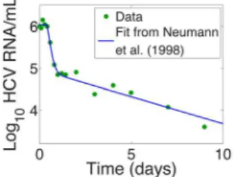
An early model of HCV infection and treatment developed by Neumann et al. [3] showed that the effectiveness of antiviral therapy in blocking HCV production from infected cells could be estimated from the kinetics and extent of viral decline during the first few days of therapy. Neumann et al. [3] also showed that if plasma HCV RNA levels were measured frequently after treatment initiation with interferon one observed a biphasic decline after a short delay when the logarithm of HCV RNA/ml was plotted versus time on treatment (Fig. 1). This type of biphasic decline has now been observed with many different types of HCV treatments including those employing PegIFN and RBV, and a variety of HCV protease and polymerase inhibitors [4–10].

The Neumann et al. model [3] assumed that there was delay before interferon became active followed by a period in which it

had constant effectiveness. Under reasonable assumptions, this leads to a model described by a set of linear, constant coefficient, ordinary differential equation that can easily be solved [3]. Models, such as that of Neumann et al., in which the drug effectiveness is constant or constant after a delay have been called constant effectiveness (CE) models [11,12]. In the case of interferon therapy we now know that the delay is caused by pharmacokinetics of the drug as well as the time needed for the drug to bind cell surface interferon receptors and cause upregulation of interferon stimulated genes, whose gene products then lead to reduced viral replication.

(2)

allows one to compare the ability of models with different numbers of parameters to fit data [15].

This study was followed by two others by Guedj et al. using VE models to analyze the HCV RNA decay kinetics observed with the nucleoside polymerase inhibitor mericitabine [16], and with the HCV nucleotide polymerase inhibitors sofosbuvir and GS-0938 [17]. In these cases, the VE model accounted for the fact that these drugs need to be triphosphorylated intracellularly to become active [18]. More recently, Canini et al. [19] used a VE model to analyze the viral kinetics seen in a different set of patients treated with the drug silibinin, which appears to have activity as both a polymerase and entry inhibitor [20,21]. In all of these studies employing VE models, numerical methods were used to solve the time-varying equations. Here, we show how a previously used and prototypic VE model can be analyzed mathematically. We obtain an analytic solution to the time-varying problem in terms of modified Bessel functions, and a set of approximate solutions involving exponential decay functions.

Models

We model HCV viral dynamics at the initiation of treatment by modifying the standard constant effectiveness viral dynamic model

of Neumann et al. [3]. For infected cells,I, and viral load,V, the model differential equations are

dI

dt~(1{g)bTV{dI dV

dt ~(1{e(t))pI{cV:

ð1Þ

We assume the number of target cells,T, is constant and takes on its pre-therapy steady-state value, T0~cd=pb. This is an approximation that is commonly made when analyzing clinical trial data obtained over a period of one or two weeks. In the case of Neumann et al. [3], it was used to analyze data collected over two weeks.

In the model given by equation (1), target cells are infected by virus,V, with mass-action infectivityb. Infected cells die at rated

per cell and virus clears at ratecper virion. The infection process may be hampered by drug treatment; the efficacy of treatment in blocking infection is given byg, 0ƒgƒ1. Infected cells produce virus at rate pper cell. Drug treatment may also interfere with viral production, with efficacy e, 0ƒeƒ1. In the constant effectiveness (CE) model the drug efficacy is assumed to be constant, e(t):e. In this case the solution for the viral load dynamics from (1) is

V(t)~V0Ae{lztz(1{A)e{l{t ð2Þ

where V0 is the viral load at t~0, l+~

(czd)+

ffiffiffiffiffiffiffiffiffiffiffiffiffiffiffiffiffiffiffiffiffiffiffiffiffiffiffiffiffiffiffiffiffiffiffiffiffiffiffiffiffiffiffiffiffiffiffiffiffiffiffiffi (c{d)2z4(1{")(1{g)cd

q

2, and A~ðec{l{Þ=

lz{l{

ð Þ[3,21]. Here we assume the drug efficacy in blocking viral production,e, is time dependent, i.e.e~e(t), with a build-up of activity to a maximum

e(t)~emax(1{e

{kt_), _ð₃_Þ

where emax is the maximum drug efficacy obtained with the concentration of drug used and the exponential scalekdetermines the speed at which the drug efficacy reaches its maximum (e(0)~0, limt??e(t)~emax). In principle, the effectiveness of treatment in blocking infection,g, could also be time dependent. Here we have chosen to ignore this possibility as no published data is available to guide such modeling efforts.

At treatment initiation (t~0) we assume the system is in steady state. Let the initial viral load, i.e., pre-treatment viral load set-point, be given byV(0)~V0. Since we assume that pre-treatment dV

dt ~0, then pI(0){cV(0)~0 and I(0)~cV0=p: Further, dI

dt~0, so that bT0V(0){dI(0)~0. Since V(0)~V0 and I(0)~cV0=p,bT0~cd=p:

Substituting forbT0, our system becomes dI

dt~(1{g) cd

pV{dI dV

dt ~(1{e(t))pI{cV:

ð4Þ

Now lety~pI,and for notational convenience letz(t)~V(t) andz0~V0

dy

dt~d(c(1{g)z{y) dz

dt~(1{e(t))y{cz

Author Summary

Fitting simple models of therapy for viral diseases, such as hepatitis C virus (HCV) or human immunodeficiency virus, to patient data has yielded significant insights into the underlying viral dynamics. In general, these models assume that, once therapy is started, the drug has a constant effectiveness. More realistic assumptions are that drug effectiveness either depends directly on the drug concentration or varies over time. Here a previously introduced varying-effectiveness (VE) differential equation model is studied in the context of HCV infection. We show that the previously-unsolved VE model can be transformed into a Bessel equation and derive an analytic solution in terms of modified Bessel functions with time-varying arguments. These analytic solutions can be more readily used to fit the model to patient data than the underlying differential equations. We also find approximate solutions and establish the asymptotic behavior of the system. Typically viral load measurements exhibit a biphasic decline after therapy initiation. We show that the rate of second phase decay is determined by the death rate of infected cells multiplied by the maximum effectiveness of therapy, whereas the rate of first phase decline may depend on multiple parameters, resulting in differing first phase declines across various HCV therapies.

Figure 1. Example of a biphasic decline of HCV, following a short delay, after initiation of interferon-atherapy att~0.Fit of Neumann et al. model (solid line) to data for Patient 1E (dots) from [3]. doi:10.1371/journal.pcbi.1003769.g001

A HCV Virus Infection Model with Time-Varying Drug Effectiveness

(3)

with initial conditionsy(0)~cz0andz(0)~z0. In the next section we will find an analytic solution for our model using this formulation.

Results

Analytic solution

We are interested in solving the system of ODEs

dy

dt~d(c(1{g)z{y) dz

dt~(1{e(t))y{cz

ð5Þ

with initial conditionsy(0)~cz0,z(0)~z0, wheree(t)is the time-dependent drug efficacye(t)~emax(1{e{kt):Assume that gv1; we treat theg~1case separately below. We can re-write this as a linear system,

d~pp dt~A(t)~pp

where ~pp(t)~(y z)T and A(t)~ {d cd(1{g) 1{e(t) {c

.

n{dimensional systems for nw1 of the form d~xx

dt~A(t)~xx have solutions, Magnus expansions, that are infinite series, which only collapse to a single term giving a closed for solution if, for anyt1, t2,A(t1)A(t2)~A(t2)A(t1)[22,23]. SinceA(t1)A(t2)=A(t2)A(t1), our system of equations (5) has no closed form solution.

However we can still recover a solution. We begin by writing the system (5) as a second-order differential equation. First, let w(t)~d(c(1{g)z{y):Then

dw

dt~d c(1{g) dz dt{

dy dt

~cd½(1{g)(1{e(t)){1y{(czd)w:

Our system of equations (5) then becomes

dy dt~w dw

dt ~cd((1{g)(1{e(t)){1)y{(czd)w:

ð6Þ

Since w~dy dt,

dw dt ~

d2y

dt2 and from (6) we recover the second order equation corresponding to the system of ODEs (5),

d2_y dt2z(czd)

dy

dtzcd(1{(1{g)(1{e(t)))y~0 ð7Þ

with initial conditionsy(0)~cz0, dy dt _t

~0

~{cdgz0:

We now employ some convenient changes in the dependent and independent variables. Lety(t)~e{(czd)t=2_u(t):_{Then (7) becomes}

d2_u dt2{

1

4ð(czd){4cdð1{ð1{gÞ(1{e(t))ÞÞu~0:

Then let x~2 ffiffiffiffiffiffiffiffiffiffiffiffiffiffiffiffiffiffiffiffiffiffiffiffiffiffi cdemax(1{g) p

e{kt=2_=k _{(recall that} _e_(t)_~ emax(1{e{kt)), so that d=dt~{(k=2)x d=dx and d2

dt2_~ (k2

4)(x2_d2

dx2_z_{x d}_{=dx), to obtain}

x2d 2_u dx2zx

du

dx{ x

2_z(czd)2{4cd eðmaxz(1{emax)gÞ k2

! u~0:

Finally letn~

ffiffiffiffiffiffiffiffiffiffiffiffiffiffiffiffiffiffiffiffiffiffiffiffiffiffiffiffiffiffiffiffiffiffiffiffiffiffiffiffiffiffiffiffiffiffiffiffiffiffiffiffiffiffiffiffiffiffiffiffiffiffiffiffi (czd)2{4cd eðmaxz(1{emax)gÞ q

=k, to simplify the equation

x2d2u dx2zx

du

dx{ x

2_z_n2

u~0: ð8Þ

Equation (8) is the modified Bessel differential equation [24], with solutions

u~c1In(x)zc2Kn(x),

whereIn(x) and Kn(x) are the modified Bessel functions of the first- and second-kind of ordern. As they represent infinite series, Bessel functions are not closed-form solutions. Note that the order

n is real: since 0ƒemaxƒ1, 0ƒgv1, the factor emaxz(1{emax)g

ð Þvaries betweenmax(emax,g)and 1. Thus

(czd)2{4cd eð maxz(1{emax)gÞ§(czd)2{4cd~(c{d)2w0:

Then sincey(t)~e{(czd)t=2_{u(t), the solution of equation (7) is}

y(t)~e{(czd)t=2_c

1Inðx(t)Þzc2Knðx(t)Þ

½ ð9Þ

wherex(t)~2 ffiffiffiffiffiffiffiffiffiffiffiffiffiffiffiffiffiffiffiffiffiffiffiffiffifficdemax(1{g) p

e{kt=2_=k:

We can use the solution (9) and the initial conditionsy(0)~cz0, dy

dt

t~0

~{cdgz0, to solve for the constantsc1,c2. Let x0~x(0)

and note thatdx

dt~{kx(t)=2, so that dy dt

t~0

~{kx0=2. Then,

noting that d

dtInðx(t)Þ~

½

(n=x(t))Inðx(t)ÞzInz1ðx(t)Þ

dx(t)

dt and

d

dtKnðx(t)Þ~

½

(n=x(t))Knðx(t)Þ{Knz1ðx(t)Þ

dx(t)

dt , y(0)~c1In(x0)zc2Knð Þx0~cz0

dy dt _t

~0 ~c1 {

czdzkn

2

In(x0){ kx0

2 Inz1(x0)

zc2 {

czdzkn

2

Kn(x0)z kx0

2 Knz1(x0)

~{cdgz0

and

c1~

cz0ðð2gd{c{d{knÞKn(x0)zkx0Knz1(x0)Þ kx0ðIn(x0)Knz1(x0)zInz1(x0)Kn(x0)Þ

,

c2~

{cz0ðð2gd{c{d{knÞIn(x0){kx0Inz1(x0)Þ kx0ðIn(x0)Knz1(x0)zInz1(x0)Kn(x0)Þ

(4)

Since In(x0)Knz1(x0)~1=x0{Inz1(x0)Kn(x0) [24] the con-stants can be written more simply as

c1~ cz0

k ðð2gd{c{d{knÞKn(x0)zkx0Knz1(x0)Þ,

c2~ {cz0

k ðð2gd{c{d{knÞIn(x0){kx0Inz1(x0)Þ: ð10Þ

To recover z(t), recall that w(t)~dy=dt and z(t)~(wzdy)=(cd(1{g)). Therefore

z(t)~ dyzdy

dt cd(1{g),

withy(t)given by (9),

dy dt~e

{(czd)t=2 _c 1 {

czdzkn

2

In(x(t)){ kx(t)

2 Inz1(x(t))

zc2 {

czdzkn

2

Kn(x(t))z kx(t)

2 Knz1(x(t))

:

Thus the viral load,z(t), is given by

z(t)~e

{(czd)t=2

cd(1{g) c1

d{c{kn

2

In(x(t)){ kx(t)

2 Inz1(x(t))

z_c₂ d{c{kn 2

Kn(x(t))z kx(t)

2 Knz1(x(t))

,

ð11Þ

where c1, c2 are given by (10), n~

=k, andx(t)~2 ffiffiffiffiffiffiffiffiffiffiffiffiffiffiffiffiffiffiffiffiffiffiffiffiffifficdemax(1{g) p

e{kt=2_=k:

Solution for general varying effectiveness model The varying effectiveness model employed above is a simplifi-cation of the more general time-varying effectiveness model,

e(t)~ 0, 0

ƒtvt0 e1z(e2{e1)(1{e{k(t{t0)), t§t0

, ð12Þ

which has been useful in cases where the viral load shows no measurable decay until timet0[6,16]. Since at low values of the effectiveness no change in viral load may be discerned due to low assay sensitivity and noise, one assumes the effectiveness has value

e1at the time viral load declines become measurable. Withe1~0, e2~emax, and t0~0 we recover the simpler form, equation (3). The analytic solution for this more general VE model can be found following the approach described above, yielding

y(t)~ cz0, 0

ƒtvt0

e{(czd)(t{t₀₎=2_c1I

nðx(t{t0)Þzc2Knðx(t{t0)Þ

½ , t§t0

wherex(t) is now given by x(t)~2 ffiffiffiffiffiffiffiffiffiffiffiffiffiffiffiffiffiffiffiffiffiffiffiffiffiffiffiffiffiffiffiffiffi cd(e2{e1)(1{g) p

e{kt=2_=k,

and the ordernisn~

ffiffiffiffiffiffiffiffiffiffiffiffiffiffiffiffiffiffiffiffiffiffiffiffiffiffiffiffiffiffiffiffiffiffiffiffiffiffiffiffiffiffiffiffiffiffiffiffiffiffiffiffiffiffiffiffi (czd)2{4cd eð2z(1{e2)gÞ q

=k(as before withe2~emax). The constantsc1,c2are still given by (10) but with x0~2

ffiffiffiffiffiffiffiffiffiffiffiffiffiffiffiffiffiffiffiffiffiffiffiffiffiffiffiffiffiffiffiffiffi cd(e2{e1)(1{g) p

=kinstead.

Analytic solution forg~1

The parameterg,0ƒgƒ1, represents the drug’s effectiveness in interfering with new cell infection withg~0indicating no efficacy and g~1indicating perfect efficacy. The analytic solution (11) assumes gv1. Perfect drug efficacy, g~1, is not a biologically reasonable assumption. However, for drugs or drug combinations with very high effectiveness in blocking viral production, viral loads fall profoundly after therapy initiation and new cell infections become rare. Under such circumstances, the solution withg~1 (i.e. no new infections after therapy is initiated) may be a reasonable approximate model [25,26].

Given g~1 the equation for infected cells, y(t), from (5) becomesdy

dt~{dy. With initial conditiony(0)~cz0the solution isy(t)~cz0e{dt. Then the equation for viral load,z(t), from (5) becomes

dz

dt~(1{e(t))cz0e

{dt_{_cz

with initial condition z(0)~z0. We can re-write this equation, using an integrating factor, as

d dt e

ct_z

ð Þ~(1{e(t))cz0e(c{d)t,

wheree(t)is given by (3). Integrating, we obtain

z(t)~z0 c(1{emax) c{d e

{dt

z cemax c{d{ke

{(dzk)t

z {c(1{emax) c{d {

cemax c{d{kz1

e{ct

~z0 c(1{emax) c{d e

{dt_{_e{ct

z cemax c{d{k e

{(dzk)t_{_e{ct

ze{ct

:

ð13Þ

For the more general varying effectiveness model given by (12), the analytic solution giveng~1fory(t)and the viral load,z(t), is

y(t)~ cz0, 0

ƒtvt0 cz0e{d(t{t0), t§t0

z(t)~

z0, 0ƒtvt0

z0

c(1{e2) c{d e

{d(t{t_0)zc(e2{e1) c{d{ke

{(dzk)(t{t₀₎

z {c(1{e2)

c{d {

c(e2{e1) c{d{kz1

e{c(t{t₀₎

, t§t0 8 > > > > > < > > > > > : z(t)~

z0, 0ƒtvt0

e{(czd)(t{t₀₎=2 cd(1{g) c1

d{c{kn

2

In(x(t{t0)){kx(t {t0)

2 Inz1(x(t{t0))

zc2

d{c{kn

2

Kn(x(t{t0))z

kx(t{t0)

2 Knz1(x(t{t0))

,

t§_t₀ 8 > > > > > < > > > > > : (13) A HCV Virus Infection Model with Time-Varying Drug Effectiveness

(5)

We note for both VE models there exist three time-scales given by the exponential decay rates{d,{d{_{k, and}{_c{d.

Transition time calculation

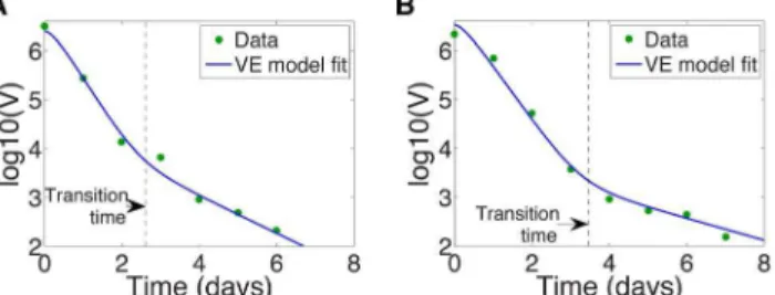
As noted before, in biologically reasonable parameter regimes this model predicts that, after initiation of antiviral therapy, viral load usually undergoes a biphasic decay, consistent with observa-tions on many different types of HCV treatments [3,6,16]. Examples are given in Figs. 1 and 2, which show the log of the viral load after treatment initiation at time t~0. The transition time between the fast- and slow- decay phases, marked by a dashed line in Fig. 2 is also of clinical interest. For example, with silibinin treatment the transition time has been shown to vary with the patient’s disease progression state (chronic HCV, compensat-ed/decompensated cirrhosis) [19].

At the transition time, the viral load curve has maximal curvature (c.f. Fig. 2). The curvature of the plane curve f(t)~log (V(t)),k(t), is given by

k(t)~ f

00_(t)

1z_ðf0_(t)_Þ2

3=2: ð14Þ

[27]. Therefore, to calculate the transition time,t, we calculate the time when the curvature k(t) is maximized. To do this we numerically solve k0_(t)_~₀ _{using the analytic solution for}

f(t)~log10(V(t)),whereV(t)~z(t)from (11).

We can use this curvature-based approach to analytically calculate the transition time for the CE model (2). Maximizing the curvaturek(t)(14) for the CE model (2), the transition timetis the solution of

for t with h~Ae{lzt_z(1_{A)e{l{t _{(in (2),} V(t)_~V

0h). The solution of (15) is lengthy and is not included here for brevity. Supporting Fig. S1 shows patient data and model fits from [3] with the transition times marked.

Parameters: Typical behaviors of different drug classes The model (1), with varying drug efficacy (12), has been used to investigate a number of drug treatments for HCV. Here we discuss therapy with four drugs: the protease inhibitors (PIs) telaprevir and

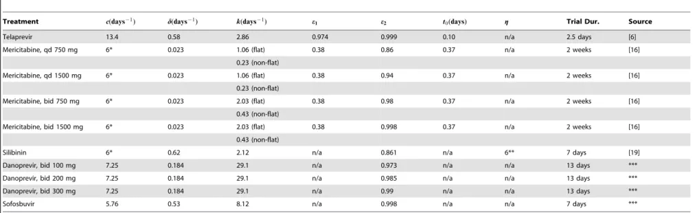
danoprevir, the nucleoside polymerase inhibitor (NPI) mericita-bine, and silibinin, a compound extracted from milk thistle seed. Silibinin is intriguing because, in addition to interfering with viral production as with the PIs and NPIs, it also appears to have some cell infection interference capabilities [21,28]. This additional capability is modeled by thegterm in (12), g~0for telaprevir, danoprevir, mericitabine, and sofosbuvir. Table 1 gives published estimates for model and drug parameters, obtained by fitting VE models to patient data, under the different treatment types, and when available different dosing regimens. The therapy durations were all two weeks or less so the assumption of a constant level of target cells was made in the primary publications from which the parameter estimates were obtained.

In the following section we analyze the analytic solution of (1), given by (11), in order to gain some insight into long- and short-term behavior. Knowledge of the magnitude and relative size of model parameters is very helpful in such analyses. Table 1 reveals that estimates from different studies are not always consistent: observe that estimates for the hepatocyte death rate d are an order of magnitude smaller for the mericitabine fits relative to the telaprevir, danoprevir, silibinin, and sofosbuvir. This discrepancy arises from the patient data used in model fitting: patients on telaprevir, danoprevir, silibinin, and sofosbuvir were treatment naı¨ve, while patients put on mericitabine had already experienced PegIFN and RBV treatment failure. Regardless, we note that

1. Final drug efficacy is quite high,e2close to 1 (e2in the general VE model (12) is equivalent toemaxin the simpler VE model (12)).

2. Viral clearance ratec&infected cell death rated(also the case

for the constant effectiveness model [3]

3. The rate of effectiveness increasekwinfected cell death rated

across all cases. We will exploit these relationships in the asymptotic analysis below.

We also note that the rate of effectiveness increase,k, can vary by orders of magnitude between drug types. For example,k~ 29:1 days{1_{in the case of danoprevir treatment,}_k[O(1) day_for telaprevir and silibinin treatments. Analysis of viral dynamics in patients on mericitabine revealed two distinct biphasic viral curve

Figure 2. HCV viral load undergoes biphasic decay upon initiation of silibinin treatment at timet~0.The transition time between the first and second phases,t, is calculated by maximizing the curvaturek(t)in equation (14), and is marked by a vertical dashed line. VE model fit of Canini et al. [19] (solid line) and HCV viral load data (dots) for (a) Patient 46, with transition timet~2:61days, and for (b) Patient 48, with transition timet~3:47days.

doi:10.1371/journal.pcbi.1003769.g002

h4L 3_h

Lt3zh 2L3h

Lt3 Lh Lt

2

z2h2 Lh Lt

3

{ Lh Lt

5

{3h3Lh Lt

L2h Lt2{3h

2Lh Lt

L2h Lt2

!2

z3h Lh Lt

3

L2h Lt2

(h2z(Lh

Lt)) 2₎(5=2)

(6)

Table 1.Model parameter estimates obtained for different drug treatments of chronic HCV.

Treatment c₍_days{1₎ _d₍_days{1₎ k₍_days{1₎ _e1 _e2 t₀₍_days₎ _g _{Trial Dur.} _Source

Telaprevir 13.4 0.58 2.86 0.974 0.999 0.10 n/a 2.5 days [6]

Mericitabine, qd 750 mg 6* 0.023 1.06 (flat) 0.38 0.86 0.37 n/a 2 weeks [16]

0.23 (non-flat)

Mericitabine, qd 1500 mg 6* 0.023 1.06 (flat) 0.38 0.94 0.37 n/a 2 weeks [16]

0.23 (non-flat)

Mericitabine, bid 750 mg 6* 0.023 2.03 (flat) 0.38 0.98 0.37 n/a 2 weeks [16]

0.43 (non-flat)

Mericitabine, bid 1500 mg 6* 0.023 2.03 (flat) 0.38 0.998 0.37 n/a 2 weeks [16]

0.43 (non-flat)

Silibinin 6* 0.62 2.12 n/a 0.861 n/a 6** 7 days [19]

Danoprevir, bid 100 mg 7.25 0.184 29.1 n/a 0.973 n/a n/a 13 days ***

Sofosbuvir 5.76 0.53 8.12 n/a 0.998 n/a n/a 7 days ***

Model parametercgives the viral clearance rate,dthe infected hepatocyte death rate,kgives the exponential scale at which the drug reaches its maximum valuee2from its minimum valuee1,t0gives the delay in the drug activity, andggives the efficacy of treatment in blocking new cell infection.

*Clearance ratecfixed atc~6days21_{from [3], not estimated.}

**Efficacy of treatment in blocking new cell infectiongfixed atg~0:6from [16], not estimated. ***Unpublished.

Notes: (i) In fitting viral load data, authors investigating telaprevir and mericitabine used the more general VE model (12), while those investigating silibinin, danoprevir, and sofosbuvir used the simple VE model (3) withemax~e2: Efficacy of treatment in blocking new cell infectiongwas only used in the silibinin model (effectively 0 in other models). (ii) qd = daily dosing, bid = bi-daily dosing. (iii) Parameter estimates derive from HCV treatment studies on patients who were treatment naı¨ve, except in the case of mericitabine, where all patients were interferon non-responders.

doi:10.1371/journal.pcbi.1003769.t001

A

HCV

Virus

Infection

Model

with

Time-Varying

Drug

Effectivenes

s

PLOS

Computational

Biology

|

www.plosc

ompbiol.org

6

August

2014

|

Volume

10

|

Issue

8

|

(7)

types across patients: the first with a flat second phase, the second with a non-flat (decaying) second phase [16]. The covariate distinguishing these two groups remains unclear. But the fits suggest the distinction lies with the parameter k, since non-flat second phases have k[O(1)_{and flat second phase patients have} k[O(10{1)[16]. In the following analysis we will considerkacross orders of magnitude.

Approximations to the analytic solution; short- and long-time behavior

The argument of the modified Bessel functions in (11) is x(t)~x0e{kt=2, wherex0~2

ffiffiffiffiffiffiffiffiffiffiffiffiffiffiffiffiffiffiffiffiffiffiffiffiffiffi cdemax(1{g) p

=k. For smallx(t)we can use the following approximations [24] for modified Bessel functions with small argumentx,

In(x)& (x=2)n

C(1zn) and

Kn(x)& 1 2 C(n)

x 2 {n

z_C({n) x 2 n

h i

, 0vnv1

1 xz x 2ln x 2

, n~₁

C(DnD) 2 x DnD ₁

2{ x2 8DnD{8

, nw₁ 8 > > > > > > > > < > > > > > > > > : :

We will neglect the n~1 case since it is highly unlikely that a set of realistic parameters will yield n~

ffiffiffiffiffiffiffiffiffiffiffiffiffiffiffiffiffiffiffiffiffiffiffiffiffiffiffiffiffiffiffiffiffiffiffiffiffiffiffiffiffiffiffiffiffiffiffiffiffiffiffiffiffiffiffiffi (czd)2{4cd eð2z(1{e2)gÞ q

=k~1exactly. The approximation fornw1is actually valid forDnDw1but sincenw0we can drop the absolute value signsD:D:Sincex(t)?0monotonically ast??we expect the approximations to hold for long times. Note that x(t)v1fortw2 ln (x0)=kandx0!1=k, so we anticipate that the approximations are appropriate even at short times for sufficiently largek. Applying the approximations to (11),

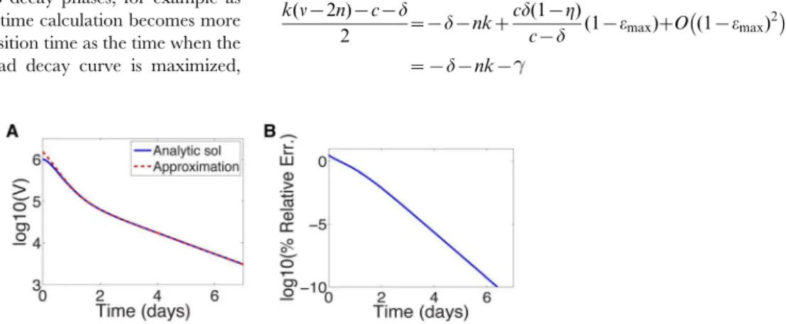
The ordern for each treatment regimen shown in Table 1 is given in Supporting Table S1 for reference. Fig. 3a shows a comparison between the approximation (16) and the analytic solution (11) for parameters characterizing silibinin (Table 1). Near t~0the error in the log of the approximation is 5% and improves significantly with increasingt(see Fig. 3b). This improvement is not surprising: the approximations are for smallx(t)andx(t)*e{kt=2 grows smaller with increasing t. Therefore we can use the approximation to gain insight into the long-time behavior.

We may also be able to use the approximation to gain some insight into the short-time behavior; although the errors neart~0

are not negligible, the approximation remains within the right order of magnitude, and away fromt~₀the slope of the solutions appear similar with these parameters, see Fig. 3a. The approxi-mation does not however capture the shoulder in the analytic solution neart~0.

Long-time behavior. From (16) we note three (for0vnv1) or four (for nw1) distinct exponential decay rates: ({kn{c{d)t=2, ({k(nz2){c{d)t=2, (kn{c{d)t=2, and, for nw1, (k(n{2){c{d)t=2. Since all parameters are positive and nw0, the slowest decay corresponds to e(kn{c{d)t=2_{. Recall} that n~

=k. If the maximum drug efficacy,emax, is close to 1,

kn{c{d

2 ~{dz

cd(1{g)

c{d (1{emax)zO (1{emax) 2

In the long term, viral load decays approximately as *e{dt_. Further, if c&d as it is for HCV (cf. Table 1) then

(kn{_c{d)=2~{d(g(1{emax)zemax), which is &{emaxd for emaxclose to 1. Not surprisingly, this is equivalent to the long-term decay rate {ed previously predicted by the CE model using similar parameter values [3].

Short-time behavior. Away from t~0 the approximate solution and analytic solution show good matching, and have similar first-phase slopes (Fig. 3). The approximation may therefore give us some insight into the first-phase decay rate. Let Arepresent the term in equation (16) that containse({kn{c{d)t=2_, Bthe term containing e({k(nz2){c{d)t=2_, _C _{the term containing} e(kn{c{d)t=2_{, and}_D_{the term containing}_e(k(n{2){c{d)t=2_._D_{is only} present in the approximation for nw1. As before, since

n~

=k and emax is near 1, to leading order the exponential decay rates are

A: {kn{c{d

2 ~{c{

cd(1{g)

B: {k(nz2){c{d

2 ~{c{k{

cd(1{g)

C: kn{c{d 2 ~{dz

cd(1{g)

D (fornw1 only): k(n{2){₂ c{d~{d{kzcd(1{g) c{d (1{emax)

zO (1{emax)2

ð17Þ z(t)&

e{(czd)t=2 cd(1{_g₎ c1

d{c{kn 21zn_C(1z_n₎

xn0e

{knt=2

{ k

2nz2_C(2z_n₎x nz2 0 e

{k(nz2)t=2

zc2 d{c{kn 2

1 2 C(n)

x0 2

{n

eknt=2_z

C({n) x0 2

n

e{knt=2

0vnv1

zk

2 C(nz1) x0

2

{n

eknt=2z_C({_n{₁₎ x0 2

nz2

e{k(nz2)t=2

,

e{(czd)t=2 cd(1{g) c1

d{c{kn 21zn_C₍₁_z_n₎

xn0e

{knt=2_{ k 2nz2_C₍₂_z_n₎x

nz2 0 e

{k(nz2)t=2

z_c2₂n_x{n 0 C(n)

d{c{kn 2

eknt=2

2 {

x2 0ek(n

{2)t=2

8n{8

nw₁

z_k_C(_nz₁₎ e knt=2

2 {

x2 0ek(n

{2)t=2

(8)

Fig. 4 shows the termsA,B,C, andDplotted against time for sibilinin parameters (nw_{1; see Table 1), compared to the exact} solution (11). Note that for long times,Cdominates (exponential decay rate&{d), as discussed above. For short times (before the transition between phases att&1) the dominant decay rate is not so obvious. It is somewhat represented byD (exponential decay rate&{d{k), as shown in Fig. 4a. But only when we add theA (exponential decay rate &{c) and C (exponential decay rate &{d) terms do we obtain a reasonable approximation (Fig. 4b). The first phase decay time scale is therefore set byd,kandc, with the initial shoulder not captured by the approximation.

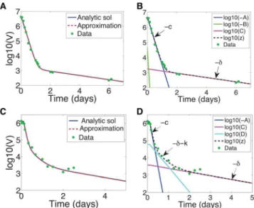
For0vnv1, Figs. 5a,b showA,B, andCplotted versus time for danoprevir parameters (see Table 1), compared to the exact solution (11). Note that for long times, again, C dominates (exponential decay rate &{d). For short times (before the transition between phases at t&2) the dominant decay rate is given by A(exponential decay rate&{c). In this case the first phase decay time scale is therefore set byc. This is not entirely surprising: askgrows large the VE model increasingly resembles the CE model, and for the CE model the first phase time scale is given by c and the second by d [3], Note that, while it’s not obvious from the log-scale in Figs. 5a,b, the initial shoulder, which is now very short, is still not captured by the approximation.

Interestingly, examining the dynamics under telaprevir treat-ment reveals that there are arguably three phases, see Figs. 5c,d. Note from Fig. 5c that the full approximation (16) is very good. As shown in Fig. 5d, the initial dynamics are well captured by A (exponential decay rate&{c), and the long-term dynamics - as always - byC(exponential decay rate&{d). But between the two there is a decay well described by D (exponential decay rate &{d{k). Numerically for telaprevir treatment these three exponential decay rates are {d~{0:58 days{1_, _{_d_{_k_~

{3:44 days{1, and{c~{13:4 days{1(see Table 1), separated by an order of magnitude, so it is not surprising that we discern three phases. We similarly discern three predicted phases under mericitabine treatment in patients characterized as ‘‘non-flat’’, see Figs. 6b,c.

When there are more than two decay phases, for example as shown in Figs. 5c,d, the transition time calculation becomes more complicated. We compute the transition time as the time when the curvature k(t) of the log-viral load decay curve is maximized,

treating the curvature maximization problem as a non-linear root finding problem, i.e. solvingk0₍_t₎_~₀_for_t_{. Multiple phase decay}

would yield multiple transition time solutions, with transition times indicating transition between decay regimes (e.g. under telaprevir treatment, dominance of c, dz_{k, or} d, as in Figs. 5c,d). Unfortunately, if the intermediate phase is not sufficiently distinct from the decay phases preceding and following it, the viral load decay may become too rounded, and our method may not give correct transition times.

The approximations (16) are valid forx(t)~x0e{kt small, and therefore we expect the approximations to improve for smallerx0 and larger k (so that x(t)?0faster). For example, the approxi-mation under telaprevir treatment is better than that for silibinin treatment (compare Fig. 3a and 5c); for telaprevir,x0~0:3and k~2:86, while for silibinin, x0~1:06 and k~2:12. In the next section we will look at a series expansion of the exact solution to show what may be missing from these approximations.

Series expansions of exact solution

The modified Bessel functions are infinite series and can be expressed as follows:

In(x)~ X

?

n~0

(x=2)2nzn

n!C(nz1zn) and Kn~

p

2 sin (pn)ðI{n(x){In(x)Þ:

For simplicity letz(t)~e{(czd)t=2_(EI

n(x)zFxInz1(x)zGKn(x)

zHxKnz1(x)) with x(t)~x0e{kt=2 (E, F, G, and H are the constant coefficients in equation (11)). Using the series expressions for Bessel functions we can re-write (11) as a series of exponential functions,

Since n~

=k and the maxi-mum drug efficacy,emax, is close to 1, the exponents can be written as

k(n{2n){c{d

2 ~{d{nkz cd(1{g)

~{d{nk{

Figure 3. Approximate and analytic solution of VE model. (a) Comparison of analytic solution (equation (11)) and the approximation (equation (16)) assuming sibilinin treatment (see Table 1 for parameters) and initial viral load of 106_IU₌_{mL. (b) Relative error in} _log

10 of approximation.

z(t)~ p

2 sin (np) x0

2 {nX

?

n~0 1 n!22n

G

C(nz1{n){

2H

C(n{n)

x20ne(k(n

{2n){c{d)t=2

z x0 2

nX

?

n~0

1

n!22n_C₍_n_z₁_z_n) Ez2nFz

p

2 sin (np)ð{Gz2nHÞ

x20ne

{(k(nz2n)zczd)t=2

(18) A HCV Virus Infection Model with Time-Varying Drug Effectiveness

(9)

{k(n

z2n)zczd

2 ~{c{nk{ cd(1{g)

c{_d (1{emax)zO(1{emax) 2

~{c{nkz ,

n~_0,1,2,_{. . .}, where is the sum of the remaining terms in the Taylor series expansion, ~_(c{d{_kn)=2[Oð1{emaxÞ. We can re-write the series expansion for the exact solution (11) as

since c[O(1{emax). As c&d, z(t)*e{dt _as _t??. Short term behavior is more difficult to discern as it depends on the magnitude of k. We can use this series expansion to evaluate parameter regimes within which the approximation (16) is valid with regards to the parameterk.

The exact solution (19) depends on the exponential decay rates {(dznk) and {(cznk) wheren~0,1,2,. . .. The approxima-tion (16) for small argumentxdepends on the exponential decay rates {d, {c, {c{k, and{d{k(the latter in the nw1case only). For these to be the most slowly decaying rates of the exact solution (19),kis constrained (recallc&d):

N

For0vnv1,dzkwczk[cvdwhich is never satisfied.

N

Fornw1,dz2kwczk[kwc{d, which is not satisfied for

any treatment regimen (see Table 1).

However, from Figs. 3, 5a, 5c, and 6a,b, it is clear that in spite of the fact that k does not satisfy the relevant condition, the approximations can be reasonably good. Direct examination of the numerical values of parameters reveals the source: the relative value ofk. A summary of how the approximations behave withk is given in Table 2.

Discussion

Viral dynamic models of infection and treatment have frequently described the effect of therapy by a parameter,e, the effectiveness of therapy, where0ƒeƒ1. For example, if therapy blocks production of new virus from infected cells, then the rate of productionpunder therapy is modeled as(1{e)p, so that when the drug is 100% effective, e~₁ and no viral production occurs. This type of formulation has been used in modeling treatment for HIV [29,30], HBV [31–33], HCV [3,7], and influenza [34]. However, the effectiveness of a drug frequently depends on its concentration and more complex models incorporating drug pharmacokinetics (PK) and drug pharmacodynamics (PD) have also made their way into viral dynamic modeling [13,14,17,35–37].

In many cases, drug concentrations are not measured and detailed PK/PD modeling cannot be performed. Nonetheless, it is clear that variations in time occur in drug concentration. Further, drug activity can also be time-dependent particular when the drug given is a ‘‘pro-drug’’ that needs to be metabolized into an active compound. For example, nucleoside or nucleotide reverse transcriptase inhibitors and polymerase inhibitors need to phos-phorylated intracellularly to become active inhibitors [38,39]. One mechanism to account for time dependent changes in drug activity is to assume that the drug effectiveness, e, rather than being constant is time dependent. Here we have studied in detail an HCV model in which the effectiveness increases with time to a maximum, assuming eithere(t)~emax(1{e{kt)or a more general

forme(t)~e1z(e2{e1)(1{e{kt), wheree2plays the role ofemax. We showed that the HCV model with time-varying effectiveness, previously used in [6,11,12,16,17], can be solved explicitly in terms of modified Bessel functions.

One reason the model equations can be solved analytically is that the assumptionT= constant is made, linearizing the mass-action infection term bTV. The assumption of constant T has typically been made when short-term (2 week or less) clinical trials are examined. However, the obtained solution may be more general, particularly for direct-acting antivirals. When therapy is very potent so the viral load rapidly decays many logs during the first days of therapy, as seen for example with daclatasvir, whereV decays 3 logs in the first 12 hrs of therapy [26], the termbTVno longer significantly influences the dynamics. Thus, after a very brief transient, whetherTis constant or not may have no practical effect on the underlying viral dynamics. Guedj et al [26] showed this to be the case for daclatasvir by finding an extremely accurate approximate solution to the viral dynamic model they used by assuming there were no new infections after therapy started, i.e. thatbTV= 0.

Plotting the solution for the viral load,V(t), on a logscale we noticed that the virus appeared to decay with time on treatment in

Figure 4. Different exponential terms in approximate solution (16) compared with the exact solution and for silibinin treatment parameters, for which nw1 (see Table 1).(a) Expo-nential terms from (16) plotted separately. (b) ExpoExpo-nential terms from (16) plotted in combined form.

z(t)~ pe

{ t

2 sin (np) x0

2 {nX

?

n~0 1 n!22n

G

C(nz1{n){

2H

C(n{n)

x2n 0e

{(dznk)t

ze t x0 2 n_X?

n~0

1

p

x2n 0e

{(cznk)t

& p 2 sin (np)

x0 2 {nX

?

n~0 1 n!22n

G

C(nz1{n){

2H

C(n{n)

x2n 0e

{(dznk)t

z x0 2

nX

?

n~0

1

p

x2₀ne{(cznk)t

(19)

(10)

a biphasic manner for certain parameters of interest. Such biphasic declines have been observed in HCV patients treated with many different therapies and the lengths of each phase and the rates of decay during each phase are of biological interest [19]. We characterized the transition between phases as the point of maximum curvature in the solution, which can be computed from the solution. However, in order to ascertain the dominant decay rates during these two observable phases, we wanted to find approximations in terms of exponentials. While the model differential equations are sufficient to fit the data, the analysis

that permits us to characterize the decay phases is only possible given the analytic solution. To this end, we examined classic approximations to Bessel functions as well as series expansions and showed that the long-time decay is dominated by the rate of loss of HCV-infected cells,d, as had previously been shown in constant effectiveness models [3]. This is not surprising since at long times, t&1=k, the drug effectiveness approaches a constant value, its

maximum. At short times, the constant effectiveness model predicts the rate of viral decay is governed by the rate of viral clearance, c. Here with the variable-effectiveness model we find

Figure 5. Approximate and analytic solution of the VE model under danoprevir (0vnv1) or telaprevir (nw1) treatment with patient data.(a,c) Approximate solution (16) compared to the analytic solution (11) for (a) danoprevir or (c) telaprevir treatment. (b,d) Different exponential terms in approximate solution compared with the exact solution, with decay phases indicated, for (b) danoprevir or (d) telaprevir treatment. Danoprevir treatment: data from patient 04-94XD (dosing 200 mg tid) in [25] with associated parameter estimates for VE model z0~3:63|106_IU₌_mL, _d_~₀_:_{33 days}{1_,_c_~₇_:_{32 days}{1_,_k_~₂₉_:_{08 days}{1_,_t0_~_{0 days,}_e

1~0, ande2~0:9996[unpublished]. Telaprevir treatment: data from patient 6 in [6] with associated parameter estimates z0~1:27|106_IU₌_mL, _d_~₀_:_{49 days}{1_, _c_~₁₅_:_{04 days}{1_, _k_~₂_:_{82 days}{1_, t0~0:1052 days,e1~0:9622, ande2~0:9972[6].

Figure 6. Approximation to viral dynamics compared to exact dynamics under mericitabine treatment, 750 mg qd,nw1.(a) For patient 92102 from [16], characterized as ‘‘flat’’. (b) For patient 92103 from [16], characterized as ‘‘non-flat’’. (c) Different exponential terms in approximate solution (16) compared with the exact solution for patient 92103, characterized as ‘‘non-flat’’. Parameter estimates from [16]: For patient 92102, z0~107_:_{14 IU}₌_mL, _d_~₀_:_{021 days}{1_, _c_~_{6 days}{1_, _k_~₀_:_{20 days}{1_, _t0_~₀_:_{5 days,} _e

1~0:27, and e2~0:91; for patient 92103, z0~106_:_{53 IU}₌_mL,_d_~₀_:_{021 days}{1_,_c_~_{6 days}{1_,_k_~₁_:_{07 days}{1_,_t0_~₀_:_{5 days,}_e

1~0:67, ande2~0:807. doi:10.1371/journal.pcbi.1003769.g006

(11)

that this need not be the case and more complex relationships between c, k and d govern the short-term behavior. Using parameters estimated in previously published drug-treatment studies we showed how different combinations of parameters govern the short-term decay for different drug therapies. For example, when k is large compared to c and d, as had been previously found for the HCV protease inhibitor danoprevir, the effectiveness rapidly approaches a constant and the first phase decline is essentially governed bycas in the constant effectiveness model. However, whenkis comparable to or small thancthis is no longer the case andkthen plays a role in determining the first phase decay. We discovered for parameters governing the HCV protease inhibitor telaprevir, where cw_kwd that three distinct exponential phases appeared to govern the viral load decay, with rates ofc,dz_{k, and}d. Viral decline under telaprevir treatment

had been previously described as biphasic [6]; it is only through the approximations to the analytic solution that the middle,dzk, phase was revealed.

The model upon which we based our analysis, while derived for HCV, applies to a number of viral infections. For example, essentially the same model can be used for protease inhibitor treatment of HIV, since HIV protease inhibitors reduce the rate of production of infectious virus. Similarly, neuraminidase inhibitors used to treat influenza A virus infection also reduce the rate of production of infectious virus and again our results would apply. HIV reverse transcriptase inhibitors act to block infection. To analyze this situation would require a generalizationq of our current model in which the parameter g rather than being constant was allowed to be time-varying. This remains an interesting problem for the future.

Supporting Information

Figure S1 Transition times between decay phases for HCV viral load decline after initiation of interferon-a therapy. Fit of Neumann et al. model (solid line) to data (dots) from [3], with transition time calculated by maximizing the curvaturek(t)(14) (cross) of the CE model (2), for patients (a) 1B, (b) 1E, (c) 1F, (d) 2D, (e) 2E, (f) 3A, (g) 3D, and (h) 3F.

(EPS)

Figure S2 Approximate and analytic solution of VE model assuming sofosbuvir treatment (see Table 1 for parameters) and initial viral load of106_{IU=mL. (a) Comparison of analytic solution} (equation (11)) and the approximation (equation (16)). (b) Relative error in log10 of approximation. Note the error near t~0 is *10%. (c) Comparison of analytic solution (equation (11)) and the approximation (equation (16)) with k~c~5:76 days21. (d) Relative error inlog₁₀ of approximation in the casek~c~5:76 days21. Note the error neart~0is*20%.

(EPS)

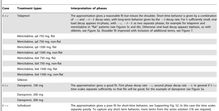
Table 2.Goodness of approximation, Eq. (16), for ranges in the parameterk.

Case Treatment types Interpretation of phases

kvc Telaprevir The approximation gives a reasonable fit but misses the shoulder. Short-time behavior is given by a combination of{cand{d{kdecay rates, with long-term behavior given by the{ddecay rate. Forksufficiently small, viral load decay appears tri-phasic, with{c,{d{kas two separate phases, for example for telaprevir and mericitabine in ‘‘flat’’ patients (see Figures 5c and 6b). Otherwise viral load decay appears biphasic, as with silibinin, see Figure 3a. Shoulder fit improved with inclusion of additional terms, see Figure 7.

Mericitabine, qd 750 mg, flat

Mericitabine, qd 750 mg, non-flat

Mericitabine, qd 1500 mg, flat

Mericitabine, qd 1500 mg, non-flat

Mericitabine, bid 750 mg, flat

Mericitabine, bid 750 mg, non-flat

Mericitabine, bid 1500 mg, flat

Mericitabine, bid 1500 mg, non-flat

Silibinin

kwc Danoprevir, 100 mg The approximation gives a good fit. First phase decay rate{c, second phase decay rate{d. In general ifkwc

time scales separate sufficiently so that fits will be good, for the example of danoprevir see Figure 5a.

Danoprevir, 200 mg

Danoprevir, 300 mg

k*c Sofosbuvir The approximation gives a poor fit for short-time behavior, see Supporting Fig. S2. In this case the time scales separate poorly. To capture any short term behavior, more terms from the series solution (19) are required.

doi:10.1371/journal.pcbi.1003769.t002

Figure 7. Truncated series solutions for the VE model compared with the exact solution (11) under silibinin treat-ment (nw1; see Table 1 for parameters).Legend: (i) Series terms with exponents{d,{d{k,{c, and{c{k terms, included in the approximation (16), from the series solution (19); (ii) Series terms with exponents from (i) and also the{d{2k and{d{3k terms missing from the approximation.

(12)

Table S1 Modified Bessel function order n for the different treatment regimens in Table 1. n is the order of the modified Bessel functions In(x) and Kn(x) in the solution (11). The approximation to the analytic solution that we use depends on whethernv1ornw1(cf. (16)).

(PDF)

Acknowledgments

We thank Harel Dahari and Jeremie Guedj for their suggestions that improved this manuscript.

Author Contributions

Conceived and designed the experiments: JMC ASP. Performed the experiments: JMC ASP. Analyzed the data: JMC ASP. Contributed to the writing of the manuscript: JMC ASP.

References

1. Schneider M, Sarrazin C (2014) Antiviral therapy of hepatitis C in 2014: Do we need resistance testing? Antiviral Res 105: 64–71.

2. Pawlotsky J (2013) Treatment of chronic hepatitis C: current and future. Curr Top Microbiol Immunol 369: 321–342.

3. Neumann AU, Lam NP, Dahari H, Gretch DR, Wiley TE, et al. (1998) Hepatitis C dynamicsin vivo_{and the antiviral efficacy of interferon-}_a_therapy.

Science 282: 103–107.

4. Dixit NM, Layden-Almer JE, Layden TJ, Perelson AS (2004) Modelling how ribavirin improves interferon response rates in hepatitis C virus infection. Nature 432: 922–4.

5. Guedj J, Neumann AU (2010) Understanding hepatitis C viral dynamics with direct-acting antiviral agents due to the interplay between intracellular replication and cellular infection dynamics. J Theor Biol 267: 330–40. 6. Guedj J, Perelson AS (2011) Second-phase hepatitis C virus RNA decline during

telapravir-based therapy increases with drug effectiveness: implications for treatment initiation. Hepatology 53: 1801–1808.

7. Rong L, Dahari H, Ribeiro RM, Perelson AS (2010) Rapid emergence of protease inhibitor resistance in hepatitis C virus. Sci Transl Med 2: 30ra32. 8. Shudo E, Ribeiro RM, Perelson AS (2008) Modelling hepatitis C virus kinetics

during treatment with pegylated interferon alpha-2b: errors in the estimation of viral kinetic parameters. J Viral Hepat 15: 357–62.

9. Shudo E, Ribeiro RM, Perelson AS (2008) Modelling the kinetics of hepatitis C virus RNA decline over 4 weeks of treatment with pegylated interferon alpha-2b. J Viral Hepat 15: 379–82.

10. Snoeck E, Chanu P, Lavielle M, Jacqmin P, Jonsson E, et al. (2010) A comprehensive hepatitis C viral kinetic model explaining cure. Clin Pharmacol Ther 87: 706–713.

11. Shudo E, Ribeiro RM, Talal AH, Perelson AS (2008) A hepatitis C viral kinetic model that allows for time-varying drug effectiveness. Antivir Ther 13: 919–26. 12. Shudo E, Ribeiro RM, Perelson AS (2009) Modeling HCV kinetics under

therapy using PK and PD information. Expert Opin Drug Met 5: 321–32. 13. Powers KA, Dixit NM, Ribeiro RM, Golia P, Talal AH, et al. (2003) Modeling

viral and drug kinetics: hepatitis C virus treatment with pegylated interferon alfa-2b. Semin Liver Dis 23 Suppl 1: 13–8.

14. Talal AH, Ribeiro RM, Powers KA, Grace M, Cullen C, et al. (2006) Pharmacodynamics of PEG-IFN alpha differentiate HIV/HCV coinfected sustained virological responders from nonresponders. Hepatology 43: 943–53. 15. Burnham KP, Anderson DR (2002) Model Selection and Multimodel Inference:

A Practical Information-Theoretic Approach. New York: Springer, 2nd edition. 16. Guedj J, Dahari H, Shudo E, Smith P, Perelson AS (2012) Hepatitis C viral kinetics with the nucleoside polymerase inhibitor mericitabine (RG7128). Hepatology 55: 1030–1037.

17. Guedj J, Pang PS, Denning J, Rodriguez-Torres M, Lawitz E, et al. (2014) Analysis of hepatitis C viral kinetics during administration of two nucleotide analogues: sofosbuvir (GS-7977) and GS-0938. Antivir Ther 19: 211–220. 18. Ma H, WR J, Robledo N, Leveque V, Ali S, et al. (2007) Characterization of the

metabolic activation of hepatitis C virus nucleoside inhibitor beta-D-29 -Deoxy-29-fluoro-29-C-methylcytidine (PSI-6130) and identification of a novel active 59 -triphosphate species. J Biol Chem 282: 29812–29820.

19. Canini L, DebRoy S, Marin˜o, Conway JM, Crespo G, et al. (2014) Severity of liver disease affects hepatitis C virus kinetics in patients treated with intravenous silibinin monotherapy. Antivir Ther: In press.

20. Dahari H, Guedj J, Perelson AS (2011) Silibinin’s mode of action against hepatitis C virus: a controversy yet to be resolved. Hepatology 54: 749. 21. Guedj J, Dahari H, Pohl RT, Ferenci P, Perelson AS (2012) Understanding

silibinin’s modes of action against HCV using viral kinetic modeling. J Hepatol 56: 1019–24.

22. Magnus W (1954) On the exponential solution of differential equations for a linear operator. Commun Pur Appl Math VII: 649–673.

23. Blanes S, Casas F, Oteo J, Ros J (2009) The Magnus expansion and some of its applications. Physical Reports 470: 151–238.

24. Spanier J, Oldham KB (1987) An Atlas of Functions. USA: Hemisphere Publishing Corporation.

25. Rong L, Guedj J, Dahari H, Coffield Jr DJ, Levi M, et al. (2013) Analysis of hepatitis C virus decline during treatment with the protease inhibitor danoprevir using a multiscale model. PLoS Comp Biol 9: e1002959.

26. Guedj J, Dahari H, Rong L, Sansone N, Nettles R, et al. (2013) Modeling shows that the NS5A inhibitor daclatasvir has two modes of action and yields a shorter estimate of the hepatitis C virus half-life. Proc Natl Acad Sci USA 110: 3991– 3996.

27. Edwards CH, Penney DE (1998) Calculus with Analytic Geometry. 5th edition. USA: Prentice-Hall Inc.

28. Blaising J, Le´vy P, Gondeau C, Phelip C, Varbanov M, et al. (2013) Silibinin inhibits hepatitis C virus entry into hepatocytes by hindering clathrin-dependent trafficking. Cell Microbiol 15: 1866–1882.

29. Perelson AS, Nelson P (1999) Mathematical analysis of HIV-1: Dynamicsin vivo_{. SIAM Rev 41: 3–44.}

30. Perelson AS (2002) Modelling viral and immune system dynamics. Nat Rev Immunol 5: 28–36.

31. Tsiang M, F RJ, Toole JJ, Gibbs CS (1999) Biphasic clearance kinetics of hepatitis B virus from patients during adefovir dipivoxil therapy. Hepatology 29: 1863–1869.

32. Lewin SR, Ribeiro RM, Walters T, Lau GK, Bowden S, et al. (2001) Analysis of hepatitis B viral load decline under potent therapy: complex decay profiles observed. Hepatology 34: 1012–1020.

33. Dahari H, Shudo E, Ribeiro RM, Perelson AS (2009) Modeling complex decay profiles of hepatitis B virus. Hepatology 49: 32–38.

34. Baccam P, Beauchemin C, Macken CA, Hayden FG, Perelson AS (2006) Kinetics of influenza A virus infection in humans. J Virol 80: 7590–7599. 35. Beauchemin CA, McSharry JJ, Drusano GL, Nguyen JT, Went GT, et al. (2008)

Modeling amantadine treatment of influenza A in vitro. J Theor Biol 254: 439– 451.

36. Dahari H, Affoso de Araujo ES, L HB, Layden TJ, Cotler SJ, et al. (2010) Pharmacodynamics of PEG-IFN-a-2a in HIV/HCV co-infected patients: Implications for treatment outcomes. J Hepatol 53: 460–467.

37. Murphy AA, Herrmann E, Osinusi AO, Wu L, Sachau W, et al. (2011) Twice-weekly pegylated interferon-a-2a and ribavirin results in superior viral kinetics in HIV/hepatitis C virus co-infected patients compared to standard therapy. AIDS 25: 1179–1187.

38. Dixit NM, Perelson AS (2004) Complex patterns of viral load decay under antiretroviral therapy: influence of pharmacokineticsand intracellular delay. J Theor Biol 226: 95–109.

39. Goldschmidt V, Marquet R (2004) Primer unblocking by HIV-1 reverse transcriptase and resistance to nucleoside RT inhibitors. Int J Biochem Cell Biol 36: 1687–1705.