Bayesian inference for two-parameter gamma distribution assuming different noninformative priors

Bayesian Inference for Two-Parameter Gamma

Distribution Assuming Different Noninformative

Priors

Inferencia Bayesiana para la distribución Gamma de dos parámetros asumiendo diferentes a prioris no informativas

Fernando Antonio Moala1,a, Pedro Luiz Ramos1,b, Jorge Alberto Achcar2,c

1_{Departamento de Estadística, Facultad de Ciencia y Tecnología, Universidade} Estadual Paulista, Presidente Prudente, Brasil

2_{Departamento de Medicina Social, Facultad de Medicina de Ribeirão Preto,}

Universidade de São Paulo, Ribeirão Preto, Brasil

Abstract

In this paper distinct prior distributions are derived in a Bayesian in-ference of the two-parameters Gamma distribution. Noniformative priors, such as Jeffreys, reference, MDIP, Tibshirani and an innovative prior based on the copula approach are investigated. We show that the maximal data information prior provides in an improper posterior density and that the different choices of the parameter of interest lead to different reference pri-ors in this case. Based on the simulated data sets, the Bayesian estimates and credible intervals for the unknown parameters are computed and the performance of the prior distributions are evaluated. The Bayesian analysis is conducted using the Markov Chain Monte Carlo (MCMC) methods to generate samples from the posterior distributions under the above priors.

Key words:Gamma distribution, noninformative prior, copula, conjugate, Jeffreys prior, reference, MDIP, orthogonal, MCMC.

Resumen

En este artículo diferentes distribuciones a priori son derivadas en una in-ferencia Bayesiana de la distribución Gamma de dos parámetros. A prioris no informativas tales como las de Jeffrey, de referencia, MDIP, Tibshirani y una priori innovativa basada en la alternativa por cópulas son investigadas. Se muestra que una a priori de información de datos maximales conlleva a una a

a

Professor. E-mail: [email protected] b

Student. E-mail: [email protected] c

posteriori impropia y que las diferentes escogencias del parámetro de interés permiten diferentes a prioris de referencia en este caso. Datos simulados per-miten calcular las estimaciones Bayesianas e intervalos de credibilidad para los parámetros desconocidos así como la evaluación del desempeño de las distribuciones a priori evaluadas. El análisis Bayesiano se desarrolla usando métodos MCMC (Markov Chain Monte Carlo) para generar las muestras de la distribución a posteriori bajo las a priori consideradas.

Palabras clave:a prioris de Jeffrey, a prioris no informativas, conjugada, cópulas, distribución Gamma, MCMC, MDIP, ortogonal, referencia.

1. Introduction

The Gamma distribution is widely used in reliability analysis and life testing (see for example, Lawless 1982) and it is a good alternative to the popular Weibull distribution. It is a flexible distribution that commonly offers a good fit to any variable such as in environmental, meteorology, climatology, and other physical situations.

LetXbe representing the lifetime of a component with a Gamma distribution, denoted byΓ(α,β) and given by

f(x|α, β) = β

α

Γ(α)x

α−1_{exp{−βx}, for allx >0 (1)}

whereα >0andβ >0 are unknown shape and scale parameters, respectively. There are many papers considering Bayesian inference for the estimation of the Gamma parameters. Son & Oh (2006) assume vague priors for the param-eters to the estimation of paramparam-eters using Gibbs sampling. Apolloni & Bassis (2099) compute the joint probability distribution of the parameters without as-suming any prior. They propose a numerical algorithm based on an approximate analytical expression of the probability distribution. Pradhan & Kundu (2011) assume that the scale parameter has a Gamma prior and the shape parameter has any log-concave prior and they are independently distributed. However, most of these papers have in common the use of proper priors and the assumption of independence a priori of the parameters. Although this is not a problem and have been much used in the literature we, would like to propose a noninformative prior for the Gamma parameters which incorporates the dependence structure of parameters. Some of priors proposed in the literature are Jeffreys (1967), MDIP (Zellner 1977, Zellner 1984, Zellner 1990, Tibshirani 1989), and reference prior (Bernardo 1979). Moala (2010) provides a comparison of these priors to estimate the Weibull parameters.

We investigate the performance of the prior distributions through a simulation study using a small data set. Accurate inference for the parameters of the Gamma is obtained using MCMC (Markov Chain Monte Carlo) methods.

2. Maximum Likelihood Estimation

LetX1,. . .,Xn be a complete sample from (1) then the likelihood function is

L(α, β|x) = β

nα

[Γ(α)]n _Yn

i=1

xα−1 i

expn−β

n X

i=1

xi o

(2)

forα >0 andβ >0.

Considering _∂α∂ logL and _∂β∂ log Lequal to 0 and after some algebric manip-ulations we get the likelihood equations given by

b

β= αb

X and logαb−ψ(α) =b log

X

∼

X

!

(3)

where ψ(k) = _∂k∂ logΓ(k)= Γ

′

(k)

Γ(k) (see Lawless 1982) is the diGamma function,

X =

Pn

i₌₁xi

n andX =

Qn i=1xi

1/n

. The solutions for these equations provide

the maximum likelihood estimators αb and βb for the parameters of the Gamma distribution (1). As closed form solution is not possible to evaluate (3), numerical techniques must used. The Fisher information matrix is given by

I(α, β) =

"

ψ′_{(α) −} 1

β −β1

α β2

#

(4)

whereψ′_{(α) is the derivative ofψ(α) called as triGamma function.}

For large samples, approximated confidence intervals can be constructed for the parametersαand β through normal marginal distributions given by

b

α∼N(α, σ2

1) andβb∼N(0, σ22), forn→ ∞ (5)

where σ2

1 =vbar(α) =b αψ_b ’α(bαb)−1 and σ 2

2 =vbar(β) =b

b

β2_ψ’(αb) b

αψ’(αb)−1. In this case, the approximated 100(1−Γ)% confidence intervals for each parameter α and β are given by

b

α−zΓ

2σ1< α <αb+zΓ2σ1 andβb−zΓ2σ2< β <βb+zΓ2σ2 (6)

3. Jeffrey’s Prior

A well-known weak prior to represent a situation with little information about the parameters was proposed by Jeffreys (1967). This prior denoted byπJ(α,β) is derived from the Fisher information matrixI(α, λ) given in (4) as

πJ(α, β)∝

p

det I(α,β) (7)

Jeffrey’s prior is widely used due to its invariance property under one-to-one transformations of parameters although there has been an ongoing discussion about whether the multivariate form prior is appropriate.

Thus, from (4) and (7) the Jeffreys prior for (α,β) parameters is given by:

πJ(α, β)∝

p

αψ′_(α)−1

β (8)

4. Maximal Data Information Prior (MDIP)

It is of interest that the data gives more information about the parameter than the information on the prior density; otherwise, there would not be justification for the realization of the experiment. Thus, we wish a prior distributionπ(φ) that provides a gain in the information supplied by data in which the largest possible relative to the prior information of the parameter, that is, which maximize the information on the data. With this idea Zellner (1977), Zellner (1984), Zellner (1990) and Min & Zellner (1993) derived a prior which maximize the average information in the data density relative to that one in the prior. Let

H(φ) =

Z

Rx

f(x|φ)lnf(x|φ)dx, x∈Rx (9)

be the negative entropy off(x | φ), the measure of the information inf(x | φ) and Rx the range of density f(x| φ). Thus, the following functional criterion is employed in the MDIP approach:

G[π(φ)] =

Z b

a

H(φ)π(φ)dφ−

Z b

a

π(φ) lnπ(φ)dφ (10)

which is the prior average information in the data density minus the information in the prior density. G[π(φ)]is maximized by selection ofπ(φ) subject toR_abπ(φ)dφ= 1. The solution is then a proper prior given by

π(φ) =kexpnH(φ)o a≤φ≤b (11)

wherek−1₌Rb

a exp

n

H(φ)odφis the normalizing constant.

Zellner (1977), Zellner (1984), Zellner (1990) shows several interesting proper-ties of MDIP and additional conditions that can also be imposed to the approach reflection given initial information. However, the MDIP has restrictive invariance properties.

Theorem 1. Suppose that we do not have much prior information available about

αandβ. Under this condition, the prior distribution MDIP, denoted byπZ(α,β), for the parameters (α,β) of the Gamma density (1) is given by:

πZ(α, β)∝ β

Γ(α)exp

n

(α−1)ψ(α)−αo (12)

Proof. Firstly, we have to evaluate the measure information H(α, β) for the

Gamma density which is given by

H(α, β) =

Z ∞

0

ln β

α

Γ(α)x

α−1_{exp{−βx}f(x|α, β)dx (13)}

and after some algebra, the result is

H(α, β) =αlnβ−ln Γ(α) + (α−1)

Z ∞

0

ln(x)f(x|α, β)dx−βE(X) (14)

withE(X) = α

β.

Since the integral functionsR₀∞uα−1_e−u_{du= Γ(α) and} R∞

0 u

α−1_log(u)e−u_{du= Γ}′_{(α), the function (14) envolving these integrals can be}

expressed as

H(α, β) =−ln Γ(α) + lnβ+ (α−1)ψ(α)−α (15)

Therefore, the MDIP prior for the parametersαandβ is given by

πZ(α, β)∝

β

Γ(α)exp

n

(α−1)ψ(α)−αo (16)

However, the corresponding joint posterior density is not proper, but surpris-ingly, the prior density given by

πZ(α, β)∝

β

Γ(α)exp

n

(α−1)ψ(α)

Γ(α)−α

o

(17)

yields a proper posteriory density. Thus, we will use (17) as MDIP prior in the numerical illustration in Section 8.

5. Reference Prior

The idea is to derive a priorπ(φ) that maximizes the expected posterior infor-mation about the parameters provided by independent replications of an experi-ment relative to the information in the prior. A natural measure of the expected information aboutφprovided by data xis given by

I(φ) =Ex[K(p(φ|x), π(φ))] (18)

where

K(p(φ|x), π(φ)) =

Z

Φ

p(φ|x) logp(φ | x)

π(φ) dφ (19)

is the Kullback-Leibler distance. So, the reference prior is defined as the prior

π(φ) that maximizes the expected Kullback-Leibler distance between the posterior distributionp(φ|x) and the prior distributionπ(φ), taken over the experimental data.

The prior densityπ(φ) which maximizes the functional (19) is found through calculus of variation and, the solution is not explicit. However, when the poste-rior p(φ | x) is asymptotically normal, this approach leads to Jeffreys prior for a single parameter situation. If on the other hand, we are interested in one of the parameters, being the remaining parameters nuisances, the situation is quite different, and the appropriated reference prior is not a multivariate Jeffrey prior. Bernardo (1979) argues that when nuisance parameters are present the reference prior should depend on which parameter(s) are considered to be of primary inter-est. The reference prior in this case is derived as follows. We will present here the two-parameters case in details. For the multiparameter case, see Berger & Bernardo (1992).

Let θ = (θ1, θ2) be the whole parameter, θ1 being the parameter of interest andθ2 the nuisance parameter. The algorithm is as follows:

Step 1: Determine π2(θ2|θ1), the conditional reference prior forθ2 assuming thatθ1 is known, is given by,

π2(θ2|θ1) =

p

I22(θ1, θ2) (20)

where I22(θ1, θ2) is the (2,2)-entry of the Fisher Information Matrix. Step 2: Normalize π2(θ2|θ1).

Ifπ2(θ2|θ1)is improper, choose a sequence of subsetsΩ1⊆Ω2⊆. . . →Ωon whichπ2(θ2|θ1)is proper. Define the normalizing constant and the proper prior

pm(θ2|θ1)respectively as

cm(θ1) =

1

R

Ωmπ2(θ2|θ1)dθ2

(21)

and

pm(θ2|θ1) =cm(θ1)π2(θ2|θ1)1Ωm(θ2), (22)

Step 3: Find the marginal reference prior πm(θ1)for θ1the reference prior for the experiment found by marginalizing out with respect topm(θ2|θ1). We obtain

πm(θ1)∝exp

n ₁ 2

Z

Ωm

pm(θ2|θ1)log

det I(θ1, θ2)

I22(θ1, θ2)

dθ2

o

Step 4: Compute the reference prior πθ1(θ1, θ2)when θ1 is the parameter of

interest

πθ1(θ1, θ2) = lim_m

→∞

cm(θ1)πm(θ1)

cm(θ∗

1)πm(θ1∗)

π(θ2|θ1) (24)

whereθ∗

1 is any fixed point with positive density for allπm.

We will derive the reference prior for the parameters of the Gamma distribution given in (1), whereα will be considered as the parameter of interest and β the nuisance parameter.

Theorem 2. The reference prior for the parameters of the Gamma distribution given in (1), where α will be considered as the parameter of interest and β the nuisance parameter, is given by:

πα(α, β) =

1 β

r

αψ′_(α)−1

α (25)

If β is the parameter of interest and αthe nuisance, thus the prior is

πβ(α, β)∝

p

ψ′_(α)

β (26)

Proof. By the approach proposed by Berger & Bernardo (1992), we find the

reference prior for the nuisance parameter β, conditionally on the parameter of interestα, given by

π(β|α) =

q

Iββ(α,β)∝ _β1 (27)

where Iββ(α,β) is the (2,2)-entry of the Fisher Information Matrix given in (4).

As in Moala (2010), a natural sequence of compact sets for (α,β) is (l1n,l2n)× (q1n,q2n), so that l1i, q1i → 0 and l2i, q2i → ∞ when i → ∞. Therefore, the normalizing constant is given by,

ci(α) =

1

Rq₂i q1i

1 βdβ

= 1

log q2i−log q1i

. (28)

Now from (23), the marginal reference prior forαis given by

πi(α) = exp

n₁

2

Z q₂i

q1i

ci(α) 1

β log

αψ′_(α)

−1 β2 α β2 dβ o (29)

which after some mathematical arrangement, we have

πi(α) =

r

αψ′_(α)−1

α exp

n₁

2ci(α)

Z q₂i

q1i

1

βdβ

o

(30)

Therefore, the resulting marginal reference prior forαis given by

πi(α)∝

r

αψ′_(α)−1

and the global reference prior for (α,β) with parameter of interestαis given by,

πα(α, β) = lim

i→∞

ci(α)πi(α)

ci(α∗_)πi(α∗₎

π(β|α)∝ _β1

r

αψ′_(α)−1

α (32)

consideringα∗_{= 1}

Similarly we obtain the reference prior considering β as the parameter of in-terest andαas nuisance. In this case, the prior is

πβ(α, β)∝

p

ψ′_(α)

β (33)

6. Tibishirani’s Prior

Given a vector parameterφ, Tibshirani (1989) developed an alternative method to derive a noninformative priorπ(δ) for the parameter of interestδ=t(φ) so that the credible interval forδhas coverage errorO(n−1_{) in the frequentist sense. This} means that the difference between the posterior and frequentist confidence interval should be small. To achieve that, Tibshirani (1989) proposed to reparametrize the model in terms of the orthogonal parameters (δ,λ) (see Cox & Reid 1987) where

δis the parameter of interest andλis the orthogonal nuisance parameter. In this way, the approach specifies the weak prior to be any prior of the form

π(δ, λ) =g(λ)pIδδ(δ,λ) (34)

where g(λ)> 0 is an arbitrary function and Iδδ(δ, λ) is the “delta” entry of the Fisher Information Matrix.

Theorem 3. The Tibishirani’s prior distributionπT(α,β) for the parameters (α,

β) of the Gamma distribution given in (1) by considering α as the parameter of interest andβ the nuisance parameter is given by:

πT(α, β)∝

1 β

r

αψ′_(α)−1

α (35)

Proof. For the Gamma model (1), we will propose an orthogonal

reparametriza-tion (δ,λ) whereδ=αis the parameter of interest andλis the nuisance parameter to be evaluated. The orthogonal parameterλis obtained by solving the differential equation:

Iββ

∂β

∂α =−Iαβ (36)

From (4) and (36) we have

α β2

∂β

∂α =

1

Separating the variables, (37) becomes the following,

1

β∂β=

1

α∂α (38)

Integrating both sides we get,

logβ=log α+h(λ) (39)

whereh(λ)is an arbitrary function ofλ.

By chosingh(λ) = logλ, we obtained the solution to (36), the nuisance param-eterλorthogonal toδ,

λ= β

α (40)

Thus, the information matrix for the orthogonal parameters is given by

I(δ,λ) =

ψ′_(δ)−1

δ 0

0 _λδ2

(41)

From (34) and (41), the corresponding prior for (δ,λ) is given by

πδ(δ, λ)∝g(λ)

r

δψ′_(δ)−1

δ (42)

whereg(λ) is an arbitrary function.

Due to a lack of uniqueness in the choice of the orthogonal parametrization, then the class of orthogonal parameters is of the form g(λ), where g(·) is any reparametrization. This non-uniqueness is reflected by the function g(·) corre-sponding to (26). One possibility, in the single nuisance parameter case, is to require that (δ, λ) also satisfies Stein’s condition (see Tibshirani 1989) for λwith

ptaken as the nuisance parameter. Under this condition we obtain

πλ(δ, λ)∝g∗(δ)

√

δ

λ (43)

Now, requiringg(λ) q

δψ′_(δ)−1

δ =g∗(δ)

√

δ

λ we have that

πT(δ, λ)∝ 1

λ

r

δψ′_(δ)−1

δ (44)

Thus, from (40), the prior expressed in terms of the (α,β) parametrization is given by

πT(α, β)∝

1 β

r

αψ′_(α)−1

α (45)

7. Copula Prior

In this section we derive a bivariate prior distribution from copula functions (see for example, Nelsen 1999, Trivedi & Zimmer 2005a, Trivedi & Zimmer 2005b) in order to construct a prior distribution to capture the dependence structure between the parametersαand β. Copulas can be used to correlate two or more random variables and they provide great flexibility to fit known marginal densities.

A special case is given by the Farlie-Gumbel-Morgenstern copula which is suit-able to model weak dependences (see Morgenstern 1956) with corresponding bi-variate prior distribution forαandβ givenρ,

π(α, β|ρ) =f1(α)f2(β) +ρf1(α)f2(β)[1−2F1(α)][1−2F2(β)], (46)

wheref1(α)andf2(β)are the marginal densities for the random quantitiesαand

β; F1(α) and F2(β) are the corresponding marginal distribution functions for α andβ, and−1≤ρ≤1.

Observe that if ρ= 0, we have independence betweenαandβ.

Different choices could be considered as marginal distributions for αand β as Gamma, exponential, Weibull or uniform distributions.

In this paper, we will assume Gamma marginal distributionΓ(a1,b1) andΓ(a2,

b2) forαandβ, respectively, with known hyperparameters a1, a2,b1 andb2. Thus,

π(α, β|a1, a2, b1, b2, ρ)∝αa1−1βa2−1exp

n

−b1α−b2β

o

×

h

1 +ρ1−2I(a1, b1α)

1−2I(a1, b1α)

i (47)

whereI(k, x) = _Γ(k)1 R₀xuk−1_e−u_{duis the incomplete Gamma function.}

Assuming the prior (47), the joint posterior distribution forα, βandρis given by,

p(α, β, ρ|x)∝ β

nα

[Γ(α)]n _Yn

i=1

xα−1 i

expn−β

n X

i=1

xi o

π(α, β|a1, a2, b1, b2, ρ)π(ρ) (48)

whereπ(ρ)is a prior distribution for ρ.

8. Numerical Illustration

8.1. Simulation Study

In this section, we investigate the performance of the proposed prior distribu-tions through a simulation study with samples of sizen= 5, n= 10 andn= 30

generated from the Gamma distribution with parametersα= 2andβ = 3. As we do not have an analytic form for marginal posterior distributions we need to appeal to the MCMC algorithm to obtain the marginal posterior distributions and hence to extract characteristics of parameters such as Bayes estimators and credible intervals. The chain is run for 10,000 iterations with a burn-in period of 1,000. Details of the implementation of the MCMC algorithm used in this paper are given below.

i) choose starting valuesα0andβ0.

ii) at stepi+ 1, we draw a new value αi+1conditional on the current αifrom the Gamma distributionΓ(αi/c, c);

iii) the candidateαi+1will be accepted with a probability given by the Metropo-lis ratio

u(αi, αi+1) = min

(

1, Γ(αi/c,c)p αi+1, βi | x

Γ(αi+1/c,c)p αi, βi| x

)

iv) sample the new valueβ_i+1 from the Gamma distributionΓ(βi/d,d);

v) the candidateβi+1will be accepted with a probability given by the Metropo-lis ratio

u(βi, βi+1) = min

(

1, Γ(βi/d,d)p αi+1, βi+1| x

Γ(βi+1/d,d)p αi+1, βi | x

)

The proposal distribution parameters c and d were chosen to obtain a good mixing of the chains and the convergence of the MCMC samples of parameters are assessed using the criteria given by Raftery and Lewis (1992). More details of MCMC in oder to construct these chains see, for example, Smith & Roberts (1993), Gelfand & Smith (1990), Gilks, Clayton, Spiegelhalter, Best, McNiel, Sharples & Kirby (1993).

We examine the performance of the priors by computing point estimates for parametersαand β based on 1,000 simulated samples and then we averaged the estimates of the parameters, obtain the variances and the coverage probability of 95% confidence intervals. Table 1 shows the point estimates forαand its respective variances given between parenthesis. Table 2 shows the same summaries forβ.

Table 1: _{Summaries for parameterα.}

α= 2 _{Jeffreys MDIP Tibshirani Reference Copula Uniform MLE}

n= 5 _{2.2529 2.1894 2.3666 2.3602 2.0909 3.3191 3.2850} (2.1640) (0.5112) (3.0297) (2.4756) (2.1987) (3.1577) (7.5372) n= 10 _{2.5227 2.2253 2.4138 2.4761 2.3068 2.9769 2.7013}

(1.3638) (0.3855) (1.3849) (1.3301) (1.2052) (1.4658) (1.8308) n= 30 _{2.1259 2.1744 2.0606 2.1079 2.0369 2.2504 2.2253}

(0.2712) (0.1910) (0.2651) (0.2728) (0.2571) (0.2829) (0.3138)

Table 2: _{Summaries for parameterβ.}

β= 3 _{Jeffreys MDIP Tibshirani Reference Copula Uniform MLE}

n= 5 _{2.9136 3.2680 3.2161 3.1058 2.7486 4.3419 5.2673} (4.2292) (1.6890) (6.1384) (4.7787) (4.2447) (5.6351) (23.1881) n= 10 3.8577 3.7727 3.6705 3.7649 3.6112 4.5186 4.2960

(3.8086) (1.5872) (3.8110) (3.6667) (3.5599) (3.7803) (5.4296) n= 30 _{3.2328 3.4255 3.1475 3.1798 3.0805 3.4633 3.4005}

(0.7950) (0.6292) (0.7861) (0.7856) (0.7453) (0.8335) (0.9163)

that, despite being widely used in the literature, they are not suitable for the Gamma distribution. As expected, the performance of these priors improves when the sample size increases.

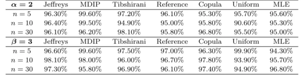
Frequentist property of coverage probabilities for the parametersαandβ have also been studied to compare the priors and MLE. Table 3 summarizes the sim-ulated coverage probabilities of 95% confidence intervals. For the three sample sizes considered here, the intervals of MDIP prior produce an over-coverage for small sample sizes while, the intervals of uniform prior and MLE seem to have an under-coverage for some cases. Coverage probabilities are very close to the nominal value when n increases.

Table 3: _{Frequentist coverage probability of the 95% confidence intervals for}αandβ. α= 2 _{Jeffreys MDIP Tibshirani Reference Copula Uniform MLE}

n= 5 _{96.30% 99.60% 97.20% 96.10% 95.30% 95.70% 95.60%} n= 10 _{96.40% 99.50% 94.90% 95.00% 95.80% 90.60% 95.30%} n= 30 _{96.10% 96.20% 98.10% 95.80% 96.80% 95.50% 95.00%} β= 3 _{Jeffreys MDIP Tibshirani Reference Copula Uniform MLE}

n= 5 _{96.60% 99.60% 97.50% 97.00% 96.30% 99.90% 94.30%} n= 10 _{98.10% 98.00% 96.00% 96.70% 97.80% 93.90% 95.70%} n= 30 _{97.30% 95.80% 96.90% 96.10% 97.40% 94.90% 96.80%}

8.2. Rainfall Data Example

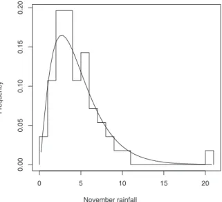
Let us assume a Gamma distribution with density (1) to analyse the data.

Table 4: _{Historical rainfall averages over last 56 years in State of São Paulo.}

0.2,3.5,2.8,3.7,8.7,6.9,7.4,0.8,4.8,2.5,2.9,3.1,4.0,5.0,3.8,3.5,5.4,3.3,2.9, 1.7,7.3,2.9,4.6,1.1,1.4,3.9,6.2,4.1,10.8,3.8,7.3,1.8,6.7,3.5,3.2,5.2,2.8,5.2, 5.4,2.2,9.9,2.1,4.7,5.5,2.6,4.1,5.4,5.5,2.1,1.9,8.8,1.3,24.1,5.4,6.2,2.9

Table 5 presents the posterior means assuming the different prior distributions and maximum likelihood estimates (MLE) for the parametersαandβ.

Table 5: _{Posterior means for parametersαandβof rainfall data.}

Uniform Jeffreys Ref-β MDIP Tibshirani Copula MLE α 2.493 2.387 2.393 2.659 2.357 2.380 2.395 β 0.543 0.516 0.517 0.641 0.510 0.515 0.518

From Table 5, we observe similar inference results assuming the different prior distributions for αand β, except for MDIP prior as observed in the simulation study introduced in the example presented in section 8.1.

The 95% posterior credible intervals obtained using the different priors for the parameters are displayed in Table 6. The MLE intervals for the parametersαand

β are given respectively by (1.56; 3.22) and (0.31; 0.72).

0 5 10 15 20

0.00

0.05

0.10

0.15

0.20

November rainfall

Frequency

Figure 1: _{Histogram and fitted Gamma distribution for rainfall data.}

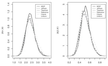
Figure 2 shows the marginal posterior densities for both parameters αand

β. We can see that the MDIP prior leads to a posterior slightly more sharply peaked for both parameters, while the other priors are quite similar, agreeing with simulated data with sample sizen= 30.

To determine the appropriate prior distribution to be used with the rainfall data fitted by the Gamma distribution, some selection criteria can be examined. These include information-based criteria (AIC, BIC and DIC) given in the Table 7 for each prior distribution.

1.0 1.5 2.0 2.5 3.0 3.5 4.0

0.0

0.2

0.4

0.6

0.8

1.0

1.2

1.4

α

p

(

α

|

x

)

MDIP Jeffreys Tibshirani Reference Cópula Uniform

0.2 0.4 0.6 0.8

0

1234

5

β

p

|

x

MDIP Jeffreys Tibshirani Reference Cópula Uniform

β(

(

Figure 2: _{Plot of marginal posterior densities for the parameters αand β of rainfall}

data.

Table 7: _{Information-based model selection criteria (AIC, BIC and DIC) for rainfall}

data.

Prior AIC BIC DIC Jeffreys 272.213 268.162 267.827 MDIP 272.247 268.196 267.502 Ref-β 272.212 268.162 267.922 Tibshirani 272.219 268.169 268.068 Copula 272.222 268.171 268.197 Uniform 272.266 268.215 267.935

8.3. Reliability Data Example

In this example, we consider a lifetime data set related to an electrical insulator subjected to constant stress and strain introduced by Lawless (1982). The dataset does not have censored values and represent the lifetime (in minutes) to failure: 0.96, 4.15, 0.19, 0.78, 8.01, 31.75, 7.35, 6.50, 8.27, 33.91, 32.52, 16.03, 4.85, 2.78, 4.67, 1.31, 12.06, 36.71 and 72.89. Let us denote this data as “Lawless data”. We assume a Gamma distribution with density (1) to analyse the data.

The maximum likelihood estimators and the Bayesian summaries forαandβ, considering the different prior distributions are given in Table 8. Table 9 shows the 95% posterior intervals forαandβ. The estimated marginal posterior distributions for the parameters are shown in Figure 3.

0.0 0.5 1.0 1.5

0.0

0.5

1.0

1.5

2.0

2.5

α

p

(

α

|

x

)

MDIP Jeffreys Tibshirani Reference Cópula Uniform

0.00 0.04 0.08 0.12

05

10

15

20

25

β

p

|

x

MDIP Jeffreys Tibshirani Reference Cópula Uniform

β(

(

Figure 3: _{Plot of marginal posterior densities for the parametersαandβ for Lawless}

data.

Tables 8 and 9 present the posterior statistics and 95% confidence intervals for both parameters resulting from the proposed priors. Again the performance of the MDIP prior clashes from the others.

Table 8: _{Posterior means for parameters}αandβ(Lawless data). Uniform Jeffreys Ref-β MDIP Tibshirani Copula MLE α 0.779 0.686 0.681 0.789 0.660 0.666 0.690 β 0.058 0.047 0.047 0.063 0.046 0.047 0.048

Table 10 shows the AIC, BIC and DIC values for all priors under investigation, with similar results as presented in Table 7 are obtained in this comparison which shows no differences using the different assumed priors.

Table 10: _{Information-based model selection criteria (AIC, BIC and DIC) for(Lawless}

data.

Prior AIC BIC DIC Jeffreys 143.125 141.236 141.409 MDIP 143.642 141.753 141.082 Ref-β 143.126 141.237 141.168 Tibshirani 143.148 141.259 141.247 Copula 143.138 141.249 141.471 Uniform 143.401 141.512 141.119

9. Conclusion and Discussion

The large number of noninformative priors can cause difficulties in the choosing one, especially when these priors does not produce similar results. Thus, in this paper, we presented a Bayesian analysis using a variety of prior distributions for the estimation of the parameters of the Gamma distribution.

We have shown that the use of the maximal data information process proposed by Zellner (1977), Zellner (1984), Zellner (1990) yields an improper posterior dis-tribution for the parametersαandβ. In this way, we proposed a “modified” MDIP prior analytically similar to the original one but with proper posterior. We also shown that the reference prior provides nonuniqueness of prior due to the choice of the parameter of interest, although the simulation shows the same performance. We have shown that the Tibshirani prior applied to the parameters of the Gamma distribution is equal to the reference prior whenαis the parameter of interest.

Besides, a simulation study to check the impact of the use of different noninfor-mative priors in the posterior distributions was also carried out. From this study we can conclude that it is necessary to carefully choose a prior for the parameters of the Gamma distribution when there is not enough data.

As expected, a moderated large sample size is need to achieve the desirable accuracy. In this case, the choice of the priors become irrelevant. However, the disagreement is substantial for small sample sizes.

Our simulation study indicates that the class of priors: Jeffreys, Reference, Tibshirani and Copula, had the same performance while the Uniform prior had worse performance. On the other hand , the “modified” MDIP prior produced the best estimations forαand β. Thus, the simulation study showed that the effect of the prior distributions can be substantial in the estimation of parameters and therefore the modified MDIP prior should be the recommended noninformative prior for the estimation of parameters of the Gamma distribution.

References

Apolloni, B. & Bassis, S. (2099), ‘Algorithmic inference of two-parameter gamma distribution’, Communications in Statistics - Simulation and Computation 38(9), 1950–1968.

Berger, J. & Bernardo, J. M. (1992), On the development of the reference prior method, Fourth Valencia International Meeting on Bayesian Statistics, Spain.

Bernardo, J. M. (1979), ‘Reference posterior distributions for Bayesian inference’, Journal of the Royal Statistical Society41(2), 113–147.

Cox, D. R. & Reid, N. (1987), ‘Parameter orthogonality and approximate condi-tional inference (with discussion)’, Journal of the Royal Statistical Society, Series B49, 1–39.

Gelfand, A. E. & Smith, F. M. (1990), ‘Sampling-based approaches to calculating marginal densities’,Journal of the American Statistical Association85, 398– 409.

Gilks, W., Clayton, D., Spiegelhalter, D., Best, N., McNiel, A., Sharples, L. & Kirby, A. (1993), ‘Modeling complexity: Applications of Gibbs sampling in medicine’,Journal of the Royal Statistical Society, Series B55(1), 39–52.

Jeffreys, S. H. (1967),Theory of Probability, 3 edn, Oxford University Press, Lon-don.

Lawless, J. (1982),Statistical Models and Methods for Lifetime Data, John Wiley, New York.

Min, C.-k. & Zellner, A. (1993), Bayesian Analysis, Model Selection and Pre-diction, in ‘Physics and Probability: Essays in honor of Edwin T Jaynes’, Cambridge University Press, pp. 195–206.

Moala, F. (2010), ‘Bayesian analysis for the Weibull parameters by using noninfor-mative prior distributions’,Advances and Applications in Statistics(14), 117– 143.

Morgenstern, D. (1956), ‘Einfache beispiele sw edimensionaler vertielung’, Mit Mathematics Statistics 8, 234–235.

Nelsen, R. B. (1999),An Introduction to Copulas, Springer Verlag, New York.

Pradhan, B. & Kundu, D. (2011), ‘Bayes estimation and prediction of the two-parameter Gamma distribution’,Journal of Statistical Computation and Sim-ulation81(9), 1187–1198.

Son, Y. & Oh, M. (2006), ‘Bayesian estimation of the two-parameter Gamma distribution’, Communications in Statistics – Simulation and Computation 35, 285–293.

Tibshirani, R. (1989), ‘Noninformative prioris for one parameters of many’, Biometrika76, 604–608.

Trivedi, P. K. & Zimmer, D. M. (2005a),Copula Modelling, New Publishers, New York.

Trivedi, P. K. & Zimmer, D. M. (2005b), ‘Copula modelling: An introduction to practicioners’, Foundations and Trends in Econometrics(1), 1–111.

Zellner, A. (1977), Maximal data information prior distributions, inA. Aykac & C. Brumat, eds, ‘In New Methods in the Applications of Bayesian Methods’, North-Holland, Amsterdam.

Zellner, A. (1984), Maximal Data Information Prior Distributions, Basic Issues in Econometrics, The University of Chicago Press, Chicago, USA.