Climatic control on the variability of flood distribution

Climatic control on the variability of flood distribution

V. Iacobellis

_{, P. Claps}

_{and M. Fiorentino}

1_{Dipartimento di Ingegneria Civile e Ambientale - Politecnico di Bari, Via E. Orabona, 4, 70125, Bari, Italy}

2_{Dipartimento di Idraulica, Trasporti e Infrastrutture Civili - Politecnico di Torino, C.so Duca degli Abruzzi 24, 10129 Torino, Italy} 3_{Dipartimento di Ingegneria e Fisica dell’Ambiente - Università della Basilicata, Contrada Macchia Romana, 85100, Italy}

Email for corresponding author: v.iacobellis@poliba.it

Abstract

The variability of the second order moments of flood peaks with respect to geomorphoclimatic basin characteristics was investigated. In particular, the behaviour of the coefficient of variation (Cv) of the series of annual maximum floods was analysed with respect to its dependence on physically consistent quantities. The results achieved were in fairly good agreement with real world observed characteristics and interesting insights on the relationship between Cv and basin size were found. It appears that Cv is controlled mainly by the climate and by some water loss features. Many observations reported in the literature show a decrease of Cv with basin area A, usually ascribed to the limited spatial extent of extreme events, which leads to a decrease with area of the Cv of areal rainfall intensity. An increase of Cv with the area is also sometimes observed for small basins. Such different behaviours were accounted for by the concurrent effect on two parameters that affect the

Cv (A) relationship, representative of the way rainfall losses and effective rainfall intensity scale with the basin area.

Keywords: floods, climate, coefficient of variation, scaling.

Introduction

This research promotes a deeper knowledge of the physical mechanisms involved in the flood generation processes, with particular regard to their use in the framework of flood frequency analysis. Yet most procedures for estimating the return period of floods are still empirical and often differ from one region to another. One problem is the relationship between the coefficient of variation (Cv) of the annual flood series and the area of the catchment. The relationships between Cv and basin area have been analysed in several studies (Smith, 1992; Gupta and Dawdy, 1995; Robinson and Sivapalan, 1997a, b; Blöschl and Sivapalan, 1997). These highlighted the complexity of patterns of Cv and the difficulty of distinguishing them because of data scatter. In particular, Blöschl and Sivapalan (1997) pointed out the role of different process controls and suggested the concept of hydrological regimes and process studies to interpret different patterns.

Available statistical procedures for flood estimation, including those based on regional analysis, usually exploit the hydrometric and pluviometric information. A marginal

role is played by basin characteristics (geology, climate, vegetation, etc.), which can be crucial to the investigation of the process whose maxima are here investigated. This research enhances the role of ancillary physical information in flood frequency estimation procedures. This approach may also lead to a deeper understanding of the process mechanisms whose composition influences the form of the distribution of the annual maximum floods.

The analysis is based on a theoretical derivation of the flood frequency function (Eagleson, 1972), a framework proposed by Iacobellis and Fiorentino (2000) and Fiorentino and Iacobellis (2001).

Theoretical framework

In the reference theoretical model (Iacobellis and Fiorentino, 2000) developed for the analytical derivation of the flood frequency distribution, an important parameter of the probability distribution of floods is the mean annual number

TCEV), represents the distribution parameter that controls the coefficient of variation Cv most strongly.

Iacobellis and Fiorentino (2000) showed that, in the case of floods generated by rainstorms, Λ_q can be related to a water loss parameter f_A by the formula:

        − Λ = Λ τ] [ exp , k A k A p q i E f ₍₁₎

in which Λ_p is the mean annual number of independent storms, E[⋅] is the expectation operator, and i_A,τ represents the average intensity of the maximum rainfall amount measured during the storm of duration τ,the lag time of the basin of surface area A; i_A,τ is assumed to be Weibull distributed with shape parameter k. Incidentally, k becomes unity when the Weibull distribution reduces to the exponential. Equation (1) is based on the simplifying assumption that the peak discharge Q_P is related to areal rainfall intensity by the equation:

Q_P = ξ ( i_a,τ - f_a ) a + q_o (2)

which is well suited for use in the framework of a theoretical model for deriving the flood distribution (Gioia et al., 2001). In the above equation, a is the variable area contributing to runoff peak, ranging from 0 to A, ξ is a routing factor less than unity, q_o is a constant base flow and f_a is the rainfall intensity threshold above which runoff is produced, as referred to variable area a. Iacobellis and Fiorentino (2000) show that Eqn. (1) can be derived from Eqn. (2) on the hypothesis that i_a,τ is a Weibull variate.

The time-space behaviour of the quantities involved is basically controlled by the commonly observed geomorphologic power-type relationship between basin lag-time τ_A and basin area A, which can be written as:

ν τ =

τa 1a , with

ν − τ =

τ_{1 A}A (3)

where τ_A is the lag-time of the basin and ν is a parameter that usually assumes values close to 0.5 (0.6 for Mitchell (1948), 0.4 for Hoyt and Langbein (1955), 0.5 for Viparelli (1963) and Troutman and Karlinger (1984)). The mean areal rainfall intensity E[i_A,τ] is usually related to A according to the power law

[ ]

τ =i A

i

E _{A, 1} (4)

where i₁ (mm h-1 _km2ε_{) is the rainfall intensity per unit area.}

Also, in the model f_A is supposed to relate to the basin area A through an equation of the type:

in which f_A represents the average water loss rate when the entire basin contributes to the flood peak. Indeed, τ_A, E[i_A], f_A, ν, ε and ε’ are characteristic features of basins.

Replacing Eqns. (4) and (5) in Eqn. (1), and considering that

[ ]

₍

[ ]

₎

the following relationship is obtained:

(

)

Λ =

Λ ε−ε

k p q i A k f 1 ' 1 1 1/

exp (7)

From Eqn. (7) it appears that the scaling relationship

Λ_q-area is clearly dependent on the values assumed by the parameters ε and ε’. The first one, ε, depends on the slope of the IDF curve and on the exponent of the geomorphological relationship τ area and usually assumes values around 0.3-0.4. The second one, ε’, is much more variable and its value may be characterised by the long term climate by way of the probable state of the basin in terms of its antecedent soil moisture conditions (Fiorentino and Iacobellis, 2001; Fiorentino et al., 2001). In particular, Fiorentino and Iacobellis (2001) elaborated Eqn. (5) into the expression: 3 3 5 . 0 2 2 1

1c A c A c

f_A =ϑ −ν +ϑ − ν+ϑ (8)

where c₁, c₂ and c₃ are coefficients depending mainly on the spatial averages of initial abstraction, characteristic sorptivity and gravitational infiltration rate, respectively. In Eqn. (8), ϑ₁,ϑ₂,and ϑ₃ are weights, ranging from 0 to 1. They are around unity in a certain climate, and approach zero elsewhere. In particular, ϑ₁ tends to prevail in arid zones, while ϑ₃ is dominant in hyper-humid climates. The second term, ϑ₂, is related to the infiltration rate through unsaturated soils. Thus, when the first term prevails, Eqn. (8) reduces to

Εqn. (5) with the value of the exponent ε’ which, according to the literature value of ν, tends to approach 0.5. In the case of prevalence of ϑ₂, ε’ is about 0.25. Finally, the dominance of the gravitational infiltration rate, in saturated soils, leads to ε’ approaching zero. The processes involved interact, depending on particular conditions of soils, land coverage and initial moisture. Knowledge of soil and climatic characteristics may lead to realistic hypotheses on how a particular value of exponent ε’ is obtained.

Study area and data set

The area under study comprises 26 gauged basins in three administrative regions in Southern Italy, i.e. Basilicata, Puglia, and Calabria (Fig. 1; Table 1).

In this area, the climate ranges from the hot-dry Mediterranean type (semi-arid or dry sub-humid) of the north-eastern sector (Puglia), to the colder and humid type of the south-western sector (Basilicata and Calabria) where the orography is more pronounced (Southern Apennine). The annual average rainfall varies from about 600 mm in Puglia to about 2000 mm in the highest parts of Basilicata and Calabria. The climatic classification, based on the Thornthwaite (1948) climatic index, is:

p p

E E h

I = − (9)

Fig. 1. Investigated region

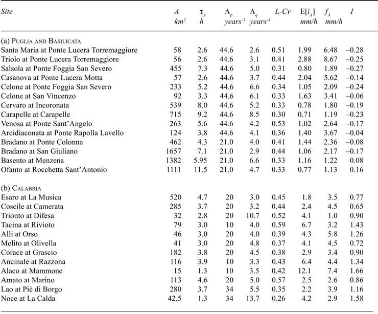
Table 1. Main morphologic and climatic characteristics of the study basins. I is the Thornthwaite climatic index

Site A τ_A Λ_p Λ_q L-Cv E[i_A] f_A I

km2 _{h years}-1 _years-1 _{mm/h mm/h}

(a) PUGLIAAND BASILICATA

Santa Maria at Ponte Lucera Torremaggiore 58 2.6 44.6 2.6 0.51 1.99 6.48 –0.28

Triolo at Ponte Lucera Torremaggiore 56 2.6 44.6 3.1 0.41 2.88 8.67 –0.25

Salsola at Ponte Foggia San Severo 455 7.3 44.6 5.0 0.31 0.80 1.89 –0.27

Casanova at Ponte Lucera Motta 57 2.6 44.6 3.7 0.44 2.04 5.62 –0.14

Celone at Ponte Foggia San Severo 233 5.2 44.6 6.6 0.34 1.05 2.09 –0.24

Celone at San Vincenzo 92 3.3 44.6 6.1 0.33 1.63 3.41 –0.06

Cervaro at Incoronata 539 8.0 44.6 5.2 0.33 0.78 1.80 –0.19

Carapelle at Carapelle 715 9.2 44.6 8.5 0.30 0.71 1.19 –0.23

Venosa at Ponte Sant’Angelo 263 5.6 44.6 4.2 0.53 1.02 2.64 –0.17

Arcidiaconata at Ponte Rapolla Lavello 124 3.8 44.6 4.1 0.36 1.40 3.67 –0.04

Bradano at Ponte Colonna 462 4.3 21.0 4.0 0.41 1.44 2.36 –0.08

Bradano at San Giuliano 1657 7.1 21.0 2.9 0.44 1.06 2.17 –0.17

Basento at Menzena 1382 5.95 21.0 6.6 0.33 1.16 1.22 0.08

Ofanto at Rocchetta Sant’Antonio 1111 11.5 21.0 4.7 0.33 0.77 1.13 0.16

(b) CALABRIA

Esaro at La Musica 520 4.7 20 3.0 0.45 1.8 3.5 0.77

Coscile at Camerata 285 3.7 20 3.2 0.44 2.4 4.5 0.65

Trionto at Difesa 32 2.8 20 10.7 0.52 4.1 1.0 0.90

Tacina at Rivioto 79 3.0 10 4.0 0.59 6.7 3.2 1.43

Alli at Orso 46 3.0 20 4.0 0.39 4.3 5.8 1.26

Melito at Olivella 41 3.0 20 4.8 0.37 4.1 4.5 0.72

Corace at Grascio 182 3.8 20 4.5 0.38 2.9 3.4 0.90

Ancinale at Razzona 116 3.9 10 3.3 0.43 6.4 4.4 1.34

Alaco at Mammone 15 1.3 10 3.5 0.42 12.1 7.4 1.66

Amato at Marino 113 4.6 20 5.0 0.57 2.5 2.6 0.86

Lao at Piè di Borgo 280 3.7 34 5.5 0.35 2.2 3.9 1.16

In which h is the mean annual rainfall and E_p is the mean annual potential evapotranspiration, calculated according to Turc’s formula (Turc, 1961), which depends on the mean annual temperature only.

ESTIMATION OF RAINFALL PARAMETERS

For the study area, regional statistical analyses of the annual maxima of hourly rainfall are available, all based on the Two Component Extreme Value (TCEV) distribution (Rossi et al., 1984). Parameters Λ₁, θ₁, and Λ₂, θ₂ of the TCEV were estimated using a Maximum Likelihood (TCEV-ML) procedure (Gabriele and Iiritano, 1994) with hierarchical estimation of parameters (Fiorentino et al., 1987), based on the homogeneous areas found in DIFA (1998), Claps et al. (1994) and Versace et al. (1989).

The estimated values of Λ_p (with Λ_p = Λ₁ + Λ₂), which can be related to the coefficient of variation of the rainfall annual maxima, are displayed in Table 1.

A regional estimation based on the Power Extreme Value-Maximum Likelihood procedure (Villani, 1993) was then applied to the same dataset, to estimate the shape factor k defined in Eqn. (1). Regional values of k were found to be 0.8 in Puglia and Basilicata and 0.53 in Calabria. The estimates of E[i_A] were obtained from the observed IDFs, exploiting the relationship between the averages of annual maxima and of the base process. The average areal rainfall intensities were estimated by means of equation:

[ ]

[

(

)

(

)

]

( )

(

)

∑

E (10)

which is valid for PEV distributed data, with p₁ the mean annual rainfall depth in 1 hour and n as the exponent of the corresponding IDF calculated for durations from 1 to 24 hours. Equation (10) includes the well-known Weather Bureau areal reduction formula, here used replacing time with the basin lag-time τ_A.

In each region (or sub-region), estimates of E[i_A] are in good agreement with the power-law relationships given in Eqn. (4). In particular, in Calabria, for basins in the Thyrrenian and Central zones i₁ = 11.5 mm h-1 _km2ε _{and ε =}

0.28 (with coefficient of determination R2 _{= 0.94), while} basins of the Jonian Zone are characterised by higher rainfall intensities, with i₁ = 28.8 mm h-1 _km2ε _{and ε = 0.32}

(R2_{= 0.98). In the other regions, the following estimates} were obtained in Puglia: i₁ = 10 mm h-1 _km2ε _{and ε = 0.39}

(R2 _{= 0.90), and in Basilicata: i}

1 = 13 mm h

-1 _km2e _and ε ₌ 2

regions are close, with a slight increase towards the north-east part of the study area.

ESTIMATION OF BASIN AND FLOOD PARAMETERS

Rainfall intensity parameters used in the model require to be considered with regard to durations corresponding to the basin lag time. In this study, lag times were either evaluated from rainfall runoff events or estimated using different empirical relations with area, according to local homogeneity found in the studies of regional flood frequency analysis. Therefore, for Calabria lag-times τ_A were taken from Versace et al. (1989); for Puglia they were taken from Ermini and Fiorentino (1994) and in Basilicata from Rossi (1974) and DIFA (1998).

The available hydrological information is completed by the estimate of the mean annual number of independent flood events, Λ_q. This parameter was estimated on all of the basins by analysing recorded series of annual flood maxima by a regional GEV-PWM procedure (Hosking and Wallis, 1993). In particular, the Λ_q values related to each series were obtained using the regional estimate of L-skewness and the at-site estimates of the L-coefficient of variation (see Iacobellis et al., 1998). Estimates of L-Cv and Λ_q are reported in Table 1. Flood data are available on the SIVAPI (1999) database.

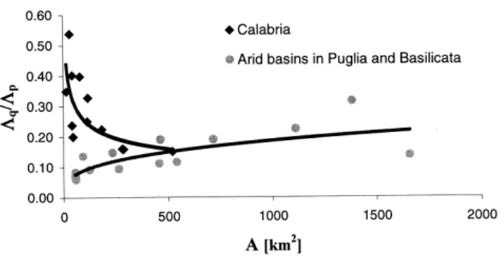
In a former application of the model to a large region of Southern Italy including Basilicata, Calabria and Puglia (Claps et al., 2001), the ratios of estimates of Λ_q and Λ_p were compared for basins of Calabria (mostly humid and permeable) and of Puglia and Basilicata (the arid ones). Figure 2 and Table 1 report the results of the analysis. A different behaviour, not dependent on the basin area, is shown by the humid basins of Puglia and Basilicata, where the flood-rainfall yield in terms of number of events is basically controlled by the climate.

The observed pattern of the ratio Λ_q/Λ_p can be explained by means of Eqn. (7). In fact, the slope of the scaling Eqn. (4) of areal rainfall intensity is substantially homogeneous over the three regions and the resulting behaviour of the ratio Λ_q/Λ_p depends on the scaling functions, Eqn. (5). In Fig. 2 two slightly humid basins with large basin area (Ofanto at Rocchetta S. Antonio and Basento at Menzena), were also included.

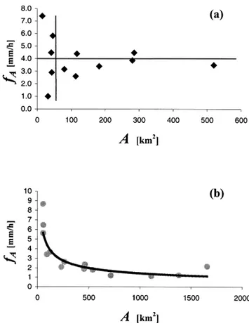
The estimates of f_A shown in Fig. 3 and Table 1 were obtained by means of Eqn. (1) rearranged into:

[ ]

(

)

k

q p A

A

k i E f

/ 1

log / 1

1 __

 

  

       

Λ Λ +

Γ

= (11)

As in Fig. 3a, in Calabria f_A is almost constant (ε’=0). Some significant deviations from this behaviour may be observed in small basins (say below 50 km2_{) where local heterogeneity} may lead to consistent oscillations of the runoff threshold. In the figure, the horizontal line represents typical behaviour of humid basins where water losses do not scale with area. The constant value represented by the horizontal line is

considerably higher than that observed in humid basins of Basilicata (Claps et al., 2001) where basins present similar climatic indices. This may reflect the fact that basins in Calabria are characterised by higher mean permeability compared to basins in Basilicata. In arid basins of Puglia and Basilicata, a clear relationship of the type shown in Eqn. (5) is observed with, ε’=0.5.

Coefficient of variation of floods and

basin area

The behaviour of the coefficient of variation Cv of annual floods was investigated with particular regard to the way it tends to scale with the basin area A. According to the probability distribution proposed by Iacobellis and Fiorentino (2000), Cv is controlled mainly by the mean annual number of floods, Λ_q, and by the shape parameter of the probability distribution of rainfall, k. In the model, Λ_q is in turn dependent on Λ_p, f_A and E[i_A], whose definitions are provided earlier. In the theoretical framework presented above, and in a region where k ad Λ_p are constant, parameters E[i_A] and f_A scale with the basin area by a power law with exponents ε and ε’ respectively. Therefore, following Eqn. (7), the relationship Cv-A depends on ε and ε’.

This result adds new arguments to the controversial question whether Cv should theoretically increase or decrease as the basin size becomes larger. In fact, many observed datasets, reported in the literature, show a decrease of Cv with area, usually ascribed to the limited spatial extent of extreme events that leads to a decrease of Cv of areal rainfall intensity. An increase of Cv with the area at small scales is also often observed. Robinson and Sivapalan (1997a) associated this pattern with the interaction between rainfall and a catchment’s characteristic timescales while Blöschl and Sivapalan (1997) indicated nonlinear runoff processes, controlled by thresholds, as the main mechanisms for the increasing of Cv, while analysing the role of several other different process controls.

The model proposed here suggests that a significant role in the control of Cv is played by the abstraction characteristics (through the parameter f_A) at the basin scale. In addition, this parameter has been shown to be strongly related to the long-term climate which drives the scaling relationship Cv-A. In particular, a double control is recognized: one related to the precipitation IDFs and their scaling with duration (through the model parameter ε); the other represented by the strong influence of the basin response in terms of the flood number ratio Λ_q / Λ_p as determined by the rainfall threshold f_A for runoff generation. In other words, the presented theoretical framework allows the relationship between the coefficient of variation Cv of

Fig. 3. Average space-time water loss intensity versus basin area A

annual floods and the basin scale to be investigated by just looking at the dependence of the parameters involved on basin scale. For example, the ε value, representative of the precipitation scaling patterns, shows a decreasing pattern versus area, producing lower Cv at larger scales. This is due to the effect of the areal averaging of precipitation and can be reproduced by the application of the classic U.S. Weather Bureau areal reduction factor to a power-law IDF (see Eqn. (10)). The same effect was also recognized by Sivapalan and Blöschl (1998), who derived a catchment’s IDF curves and related areal reduction factors based on the spatial correlation structure of rainfall.

As a first approximation, it can be assumed that k = 1, corresponding to the hypothesis of exponential distribution of rainfall intensity. In this case the proposed model leads to a distribution that, under a wide range of situations, is not very far from a simple Gumbel distribution (EV1).

The standard form of the Gumbel distribution’s cdf, written as

( )

  

 

   

 

α ξ − − −

= Q

Q

Fq exp exp

(12)

with variance σ2

q and mean µq values respectively

6

2 2 2 ₌π α

σq , µq =ξ+0.5771α (13)

can also be expressed as the distribution of the maximum of a Poissonian number of exponentially distributed peaks over a threshold x₀ →0. In this case the form of the EV1 appears as (Stedinger et al., 1992)

( )

  

 

      − Λ − =

α

Q Q

Fq exp qexp

(14)

where α is the mean of the exponential variable and Λ_q is the rate of the Poisson process. Gumbel parameters α and ξ can be thus related to Λ_q through the moments (Eqn. (13)) of the distribution, providing

( )

ξ . (15)

Then the following relation between Cv and Λ_q arises:

5771 . 0 log

28255 . 1

+ Λ = µ σ =

q q

q

Cv (16)

In terms of the parameters of the proposed models, replacing Eqn. (1) into (16) produces:

5771 . 0 ln

28255 . 1

'

1

1 ₊

− Λ =

ε − ε

A i f Cv

p

(17)

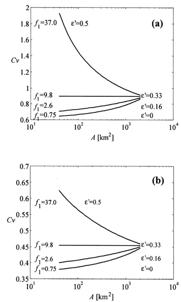
which represents the above-mentioned Cv-A relationship. In Fig. 4, as an example, the form assumed by the relationship of Eqn. (17) is shown for two different Poisson rates: Λ_p= 5 and Λ_p=20. The other parameter values assumed are i₁ = 13 mm h-1 _km0.66_, ε _{= 0.33 and f}

A = 0.75 mm/h, for A=2500 km2_{. The patterns shown in Fig. 4 for different} values of ε’ (0, 0.16, 0.33 and 0.5) producing corresponding values of f₁ (0.75, 2.6, 9.8 and 37 mm h-1 _km2ε’_{), highlight} that the scaling relationship Cv-A, the other quantities constant, is significantly dependent on the values ε and ε’ and their difference.

Fig. 4. Coefficient of variation of flood annual maxima versus basin area A, according to equation (17), with i1= 13 mmh

Commenting on Fig. 4 and taking into account the typical values of ε’ presented in the previous section, it is possible to observe that Cv decreases with the basin area A in arid basins, where the prevailing runoff generation mechanism is of the infiltration excess (Horton type) and f_A tends to scale with A raised to the power ε’ = 0.5 (for a more general comment on this topic, see also Fiorentino and Iacobellis, 2001). Conversely, in humid and vegetated basins, where the prevailing runoff generation mechanism is saturation excess (Dunne type), and ε’ tends to zero, Cv may increase as the basin area increases. On the other hand, Fig. 4 also points out that Eqn. (17) shows a more significant sensitivity of Cv to A when ε’ is greater than ε. This may provide an explanation for the fact that in the real world a negative scaling of Cv with the basin area A seems to prevail.

A relationship analogous to Eqn. (17) is derived in terms of L-moments (λ₁, λ₂, ...) and L-moment ratios, defined as (Hosking, 1990):

1 2/λ

λ

τ = ; τr=λr/λ2; r = 3, 4, ... (18)

The latter have meaning of coefficient of variation (L-cv), skewness (L-ca) and kurtosis (L-k) respectively: τ, τ₃, τ₄.

L-moments unbiased estimators are expressed by:

l_r p_{r k}b_k

k r

+ =

=

∑

0 ,

* with

(

)(

) (

)

(

)(

) (

)

b n j j j k

n n n k x

k j

j n

= − − −

− − −

−

=

∑

1

1

1 2

1 2

... ...

(19)

where x_j, j = 1,...,n is the ordered finite sample and n is the observation length; b_k and l_r are unbiased estimators of β_k and λ_r (β_k are probability weighted moments introduced by Greenwood et al., 1979), while t=l₂ / l₁ and t_r=l_r / l₂ are consistent but not unbiased estimators of τ and τ_r.

Hence, Eqn. (15) is replaced by (Stedinger et al., 1992)

( )

λ (20)

and the following expression of L-Cv is obtained:

( )

5771 . 0 ln

2 ln

'

1

1 ₊

− Λ = −

ε − ε

A i f Cv

L

p

(21)

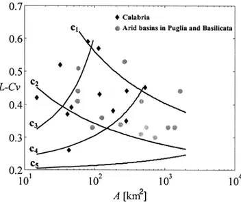
Figure 5 presents four curves obtained by means of Eqn. (21) for typical values of parameters estimated within the investigated region (Table 1).

In the figure there are two main groups of basins, presenting two classes of relations in the (A, L-Cv) plane. Arid basins in Puglia and Basilicata present a clear reduction

Fig. 5. L-Coefficient of variation of flood annual maxima versus basin area A according to equation (21), with different parameters; arid basins of Puglia and Basilicata (c

1 and c2): i1 = 10 mmh -1_km0.8_,

f1= 37mmh

-1_{km, ε = 0.4, ε’=0.5 and Λ}

p=20 (c1), Λp= 44 (c2);

Calabria (c

3, c4 and c5): i1 = 11.1 mmh

-1_km0.56_{, ε = 0.28, ε’=0,} Λp=20 and f1= 7.5mm/h (c3), f1= 4mm/h (c4) and f1= 1mm/h (c5).

of f_A with area (Fig. 3b), which for typical values of other parameters in that region, allows them to demonstrate a decreasing relation of L-Cv with area. Curves c₁ and c₂ were built for different values of Λ_p, which in fact delimit two homogeneous regions with respect to that parameter. Humid basins (in Calabria) present an almost constant f_A but with high variability for small basins. Three values of the latter parameter were used to build curves c₃ to c₅ that represent different groups of basins in the region. Both the classes of (A, L-Cv) curves are intended as reference curves representative of typical patterns but are not fitted from the data.

Conclusions

In this study the variability of the coefficient of variation Cv of flood peaks annual maxima was investigated with particular regard to the way it tends to scale with the basin area A. The analysis was developed within the framework of the theoretical distribution of floods proposed by Iacobellis and Fiorentino (2001). According to this distribution, Cv is controlled mainly by the mean annual number of floods, Λ_q and by the shape parameter k of the (PEV) probability distribution of rainfall. In the model, Λ_q is in turn dependent on parameters Λ_p, f_A and E[i_A]. In regions where k and Λ_p are constant, E[i_A] and f_A scale with the basin area. Therefore, the relationship Cv-A depends on the scaling parameters ε and ε’ respectively related to the structure of precipitation and to a combination of soil and climate parameters. This result suggests that the Cv behaviour is controlled by the abstraction characteristics at the basin scale, as well as by long-term climate.

The decrease in Cv with area which is often observed, is reproduced correctly where the infiltration excess (Horton type) mechanism dominates, as in arid and impermeable basins, or whenever ε < ε’. On the other hand, an increase of Cv with area can be justified in humid and vegetated basins and is consistent with saturation excess (Dunne type) runoff.

When examining real-world data, the sample variability of L-moments and of the model parameters can play a marked role, as well as the departure of the flood frequency distribution from the EV1 model, which drives the Cv-Λ_q relation.

Finally, non-linear effects due to the superposition of different mechanisms of runoff generation, which add complexity to the scaling properties of Cv, are not taken into account in this paper.

Acknowledgements

This work was supported by funds granted by the Consiglio Nazionale delle Ricerche – Gruppo Nazionale per la Difesa dalle Catastrofi Idrogeologiche and by MURST (Italian Ministry of Education and University), project ECAPI. Comments and suggestions of two anonymous reviewers are gratefully acknowledged.

References

Blöschl, G. and Sivapalan, M., 1997. Process controls on regional flood frequency: Coefficient of variation and basin scale, Water Resour. Res.,33, 2967–2980.

Claps P., Copertino, V.A., Ermini, R. and Fiorentino, M., 1994. Analisi regionale dei massimi annuali delle precipitazioni di diversa durata (in Italian). In: Valutazione delle piene in Puglia

report, Dipartimento di Ingegneria e Fisica dell’Ambiente and Gruppo Nazionale per la Difesa dalle Catastrofi Idrogeologiche, Univ. della Basilicata, Potenza, Italy.

Claps,P., Fiorentino, M. and Iacobellis, V., 2001. Regional flood frequency analysis with a theoretically derived distribution function, Proc. of the 2nd _{Plinius Conference on Mediterranean}

Storms, European Geophysical Society, Siena, Italy, 16–18 October 2000 (in press),

DIFA, 1998. Valutazione delle Piene in Basilicata (in Italian), report, Dipartimento di Ingegneria e Fisica dell’Ambiente and Gruppo Nazionale per la Difesa dalle Catastrofi Idrogeologiche, Univ. della Basilicata, Potenza, Italy.

Eagleson, P.S., 1972. Dynamics of flood frequency, Water Resour. Res.,8, 878–898.

Ermini, R. and Fiorentino, M., 1994. I tempi di ritardo caratteristici dei bacini idrografici. In: Valutazione delle Piene in Puglia, report, Dipar-timento di Ing. e Fis. dell’Ambiente, Univ. della Basilicata, Potenza, Italy.

Fiorentino, M. and Iacobellis, V., 2001. New insights about the climatic and geologic control on the probability distribution of floods. Water Resour. Res.,37, 721–730.

Fiorentino, M., Gabriele, S., Rossi, F. and Versace, P., 1987. Hierarchical approach for regional flood frequency analysis. In: Regional flood frequency analysis, V.P. Singh (Ed.), D. Reidel, Norwell, MA., 35–49.

Fiorentino, M., Margiotta, M.R. and Iacobellis, V., 2001. Effects of Climate and Antecedent Soil Moisture on the Areal Average Abstraction Losses. Proc. XXIX IAHR Congress, September 16-21, 2001.

Gabriele, S. and Iiritano, G., 1994. Alcuni aspetti teorici ed applicativi nella regionalizzazione delle piogge con il modello TCEV, (in Italian), GNDCI – Linea 1 U.O. 1.4, Pubblicazione N. 1089, Rende (Cs).

Gioia, G., Iacobellis,V. and Margiotta, M.R., 2001. Assessment of a simplified runoff model for the theoretical derivation of the probability distribution of floods. In: The Extremes of the Extremes: Extraordinary Floods, Arni Snorrason et al. (Eds.) IAHS Publ. no. 271.

Greenwood, J.A.,Landwehr, J.M., Matalas, N.C. and Wallis, J.R., 1979. Probability weighted moments: Definition and relation to parameters of several distributions expressable in inverse form. Water Resour. Res., 15, 1049–1054.

Gupta, V. K. and Dawdy, D.R., 1995. Physical interpretations of regional variations in the scaling exponents of flood quantiles,

Hydrol. Process., 9, 347–361.

Hosking, J.R.M., 1990. L-moments: Analysis and estimation of distributions using linear combinations of order statistics, J. Roy. Stat. Soc., B 52, 105–124.

Hosking, J.R.M. and Wallis, J.R., 1993. Some Statistic useful in Regional Frequency Analysis, Water Resour. Res., 29, 271–281. Hoyt, W.G. and Langbein, W.B., 1955. Floods. Princeton

University Press, NJ. 469 pp.

Iacobellis, V. and Fiorentino, M., 2000. Derived distribution of floods based on the concept of partial area coverage with a climatic appeal. Water Resour. Res., 36, 469–482.

Iacobellis, V., Claps, P. and Fiorentino, M., 1998. Sulla dipendenza dal clima dei parametri della distribuzione di probabilità delle piene, (in Italian), In: Proc. XIV Convegno di Idraulica e Costruzioni Idrauliche, Univ. of Catania, Catania, Italy. II, 213– 224.

Robinson, J.S. and Sivapalan, M., 1997a. An investigation into the physical causes of scaling and heterogeneity of regional flood frequency. Water Resour. Res., 33, 1045–1059

Robinson, J.S. and Sivapalan, M., 1997b. Temporal scales and hydrological regimes: Implications for flood frequency scaling.

Water Resour. Res., 33, 2981–2999.

Rossi, F., 1974. Criteri di similitudine idrologica per la stima della portata al colmo di piena corrispondente ad un assegnato periodo di ritorno. Paper presented at the XIV Convegno di Idraulica e Costruzioni Idrauliche, Univ. of Naples, Naples, Italy. Rossi, F., Fiorentino, M. and Versace, P., 1984. Two component

extreme value distribution for flood frequency analysis. Water Resour. Res., 20, 847–856.

Sivapalan, M. and Blöschl, G., 1998. Transformation of point rainfall to areal rainfall: Intensity-duration-frequency curves.

J. Hydrol., 204, 150–167.

SIVAPI, 1999. Sistema Informativo per la Valutazione delle piene in Italia. (http://www.gndci.cs.cnr.it./sivapi).

Smith, J.A., 1992. Representation of basin scale in flood peak distributions. Water Resour. Res.,28, 2993–-2999.

Stedinger, J.R., Vogel, R.M. and Foufoula-Georgiou, E., 1992. Frequency analysis of extreme events. In: Handbook of Hydrology, D.R. Maidment (Ed.), Chap. 18, McGraw-Hill. Thornthwaite, C.W., 1948. An approach toward a rational

classification of climate. Amer. Geograph. Rev., 38, 55–94. Troutman, B.M. and Karlinger, M.R., 1984. Unit hydrograph

approximations assuming linear flow through topologically random channel networks. Water Resour. Res., 21, 743–754. Turc, L., 1961. Estimation of irrigation water requirements,

potential evapotranspiration: a simple climatic formula evolved up to date. Ann. Agronomy, 12, 13–14.

Versace, P., Ferrari, E., Gabriele, S. and Rossi, F., 1989.Valutazione delle piene in Calabria (in Italian). CNR-IRPI, Geodata. Villani, P., 1993. Extreme flood estimation using Power Extreme

Value (PEV) distribution. Proc. IASTED International Conf.,

Modeling and Simulation, M.H. Hamza (Ed.), Univ. of

Pittsburgh, Pittsburgh, PA. 470–476.