Approximate analytic expression for the eigenenergies of the anharmonic oscillator V(x)=Ax6+Bx2

Approximate

analytic expression for

the

eigenenergies

of

the

anharmonic

oscillator

V(~)

=

A.

~'+

H~'

A.de Souza Dutra* and A.

S.

de Castrot

Departmento de Eisica e quimica, Uniuersidade Estadual Paulista, Campus de Guaratingueta, Caiza Postal 205, 12500-000 Guaratingueta, Sao Paulo, Brazil

H. Boschi-Filho~

Instituto de Fxsica, Universidade Federal doRio de Janeiro, Cidade Universitaria, Ilha do Fundao,

|

aiba Postal 68588,

219/5 970-Rio de Janeiro, Rio de Janeiro, Brazil (Received 1July 1994)

An approximate analytic expression for the eigenenergies of the anharmonic oscillator V(x)

=

Ax

+

Bx

is introduced, starting from particular analytic solutions which are valid when certain

relations between the parameters A.and

B

are held.

PACS number(s): 03.65.Ge, 02.60.

—

x, 02.70.

—

c

I.

INTRODUCTION

A problem that has been challenging physicists and mathematicians for years is the search for analytic so-lutions for anharmonic oscillators. As

it

is well known,

the general solution for this problem has not yet been found; however, particular analytic solutions have been

discovered when the potential parameters obey certain relations.

It

is important

to

note

that

these particular analytic solutions donot cover the entire spectrum

of

the

problem even in the case

of

simpler examples. Potentials

with these characteristics are then called partially alge-brized or quasi-exactly-solvable [1—

21].

Since the complete spectra of anharmonic oscillators

are not analytically known it is usual

to

implement

nu-merical methods

to

find the energy eigenvalues. This is

quite satisfactory for

a

particular potential with all its parameters 6xed

to

certain numerical values. The price paid in this approach is

that

one cannot in general write

a

closed expression for the relevant functions related

to

the solutions

of

the problem as the eigenenergies or wave

functions even for

a

more restricted class

of

potentials.

Clearly there is

a

gap between these two approaches and in this paper we want

to

make some eKort in the

di-rection

of

connecting them. Todo this we will start with

the partial analytic solutions known for the double-well

potential

V(x)

=

Axe

₊

_{Hx~ (A} & O,

R

(

0) including

their energy spectrum but only in a recurrence relation

form and then obtain its numerical counterpart. From

these numerical data we establish relations between the

energy

E

and the parameters A and

B.

Apart &om itsintrinsic interest, the double-well poten-tial also plays an important role inthe quantum study

of

the tunneling time problem [22],in spectra

of

molecules such as ammonia and hydrogen-bonded solids _[23],and in field theory [24]. In fact, the double-well potential that will be focused on in this work might be used as

a

potential model for quark con6nement in quantum chro-modynamics [25]. On the other hand, by performing suitable point-canonical transformations,

it

is possible

to

show that there is

a

mapping from the potential

of

Rydberg atoms in uniform magnetic 6elds into that of

some double-well potentials [26].

Both

these problems

are generally studied in terms

of

standard perturbative approaches.

It

should be very pro6table

to

obtain some analytical information, even though approximately, like

that

proposed here.

This paper is organized as follows. In

Sec.

II

we

re-view the algebraic approach for the potential

V(x)

Ax

+

Bx

and determine the energy relations for the

6rst

analytic eigenfunctions. In

Sec.

III

we take these energy relations, which are valid when A and

B

satisfy

a

constraint relation, and interpolate them numerically.

Then we obtain an expression for the energy as

a

function

of

A,

B

and n, the principal quantum number, forn &

3.

In

Sec. IV

we show that these results can be extended

to

higher excited states and in

Sec.

V we present our 6nal considerations.

II.

ALGEBRAIC APPROACH

In this section we review the analytic properties

of

the

Schrodinger equation

—

—

0"

₊

VO'

=

E4'

2

for the sextic anharmonic potential [7,21]

V(z)

=

Axs

₊

Rx',

A &

0,

(2)

*Electronic address: dutragrtggg

.

uesp.ansp. br

t_{Electronic address: castrogrtQQQ}

_.

_{uesp.ansp. br}

~_{Electronic address: boschiOufrj. bitnet}

obtaining explicitly the expressions for the energy

corre-sponding

to

the ground and lowest excited

states.

As is

well known, the Schrodinger equation for this potential can be solved by writting the wave function as

@(x)

@(x)

—42A e /4

Ã

@even(x)

—

)

ajx

Oy2i~ ~~

(4)

or

N

4' _gg(x)

=

)

_a,

.

x'.

1y3i~ ~ ~

The exact solutions are only possible when certain

rela-tions among the coeffients a~'s are satis6ed, which can be written as recurrence relations

where the remaining function

4'(x)

must be

a

polynomial

of

definite parity:

N=3,

N=4,

N=5,

N=6,

N=7,

N=8,

N=9,

N=11,

0

= E

—

6m2A,

0

= E

E2

—

16

2A

0=E

E

—

32 2A

O

=

E'

—

6OE'v'2A+

36OA,

0

= E

—

100E v'2A+

1512A,

0

=

E

~

E

—

180E

V

2A+

58882),

0

= E E

—

240E

2A+

16128A

0

= E

—

350E

v 2A

+

41432E

A

—

_{162000 ~2As1}~,

0

= E

—

490E

v 2A

+

91160

E

A

—

₈₃₁₆₀₀

_&2A ~

_.

(11)

(12)

(13)

(i4)

(i5)

(16)

(17)

(18)

(19)

E

a~

+

(N

+

2

—

j

₎

+2A

a~

(j

+

2)

(j

+

1)

(6)

where

E

is the energy eigenvalue. Note

that

for

j'

)

N

all a~1

=

0.

This equation can be used

to

obtain the

energy equation

aiv

E

—

2v'2A aN g

—

—

0.

(7)

These restrictions imply

that

the potential parameters A and

B

must be related by

B =

—

u'2A

_(N

₊

~~),

in order

to

ensure

exact

solvability. One should observe

that

the parameter

B

is always negative. Therefore, we

would not expect any kind

of

harmonic oscillator limit, in

the case

of

arbitrary parameters, when A goes

to

zero. In order

to

take into account the casewhere

B

is positive, we

suppose that some sort

of

analytical continuation should

be done. Indeed,

a

particular case of the above mentioned

potential has been studied, regarding problems related

to

analytical continuations

of

their parameters by Bender

and Turbirner [27].Moreover some discontinuities in the

eigenenergy spectra

of

some polynomial potentials have

been reported by Panday and Varma [28]. Thus

it

is quite clear

that

any limit and extrapolations should be

done very carefully. In fact, the potential

V(x)

=

Axe

+

Bx

belongs

to

a

general family

of

quasi-exactly-solvable

potentials [7,21] for which partial analytic solutions are known when its parameters satisfy constraint conditions.

Choosing

a

certain value for

N,

we fix also the number

of

exact levels

that

can be found in this approach: 1

+

N/2

levels when

N

is even and

(1+

N)/2

levels when

N

is

Qdd.

The expressions for the energy eigenvalues for the first values

of N,

corresponding

to

the potential

_(2),

may be

expressed as

III.

ANALYTIC-NUMERICAL

APPROACH

In order

to

6nd an analytic expression which gives ap-proximate values for the eigenenergies for arbitrary pa-rameters [not only for those satisfying

(8)]

we use

a

nu-merical method

of

adjustment and interpolation starting

with the analytical eigenenergies for parameters which satisfy

(8).

These two variables are then fitted through

a

polynomial

of

arbitrary degree which best fit resulted

in one

of

third degree:

E =

a+bB+eB

+dB

Noting that the coefficients

a,

b, c, and d must depend on the parameter A and the principal quantum number

n, we write

E

=a

(A)+b

(A)

B+c„(A) B +d

(A.₎

B

.

(20) The next step is

to

find out these dependences explic-itly. The best fit in this case is obtained by single power functions for each coefficient which read

a„(A)

=

c5.

„A

2

b„(A)

=

P„A

(21)

(22)

c„(A)

=

p„A

(23)

This method may be applied for an arbitrary

N,

but in

practice this is difficult

to

handle. In this analysis, we

6rst

confine ourselves

to

N

&

11

with the advantage

of

6nding algebraic equations for

E

which can be reduced

to

the third power (for the energy squared) so

that

their exact roots may be easily obtained. Finally, we obtain the complete dependence

of

E

on the parameters A,

B,

and

n.

In

Sec. IV

we extend this discussion

to

N

=

20

and

30,

when only numerical solutions are possible.

N

=Oor1,

N=2,

0

=E,

0

= E

—

2V'2A,

(9)

t'~

)'

+b„

A)

(25) The behavior

of

the coefficients

_{n, P,}

_p, and b against n

results in the polynomials

E„=

A ~

n„+P„

A

₍

_A)

Keeping

Eqs.

(20) and

₍₂₁₎

—(24) in mind, it is possible

to state

that the energy can be written as a function

of

parameters A and

B

and the quantum nuxnber

n:

The best fitting for these points leads

to

the equation

—

_0.

₄₈₂₉₈₆

₊

7.

44313

x

10 2n

—

_3.

_{91992 x}

_{10 n}

+

1.

30664

x

10 n

.

(3

Analogously, for

N

=

30 we find

(/2A

=

10

is)

a

polynomial equation

of

eigth power for the energy squared, which leads

to

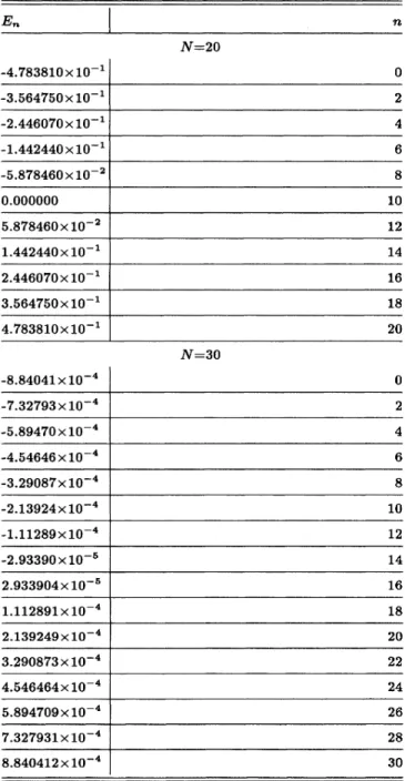
the eigenvalues also shown in

Table

II.

These data lead

to

the equation

a

=

0.

2310

+

2.

995n

—

1.

466n

+

0.

4490n (26)

_E„~~2~

_io,

e ——

—

8.

95776

x

10

P„=

(

—

1.224+ 9.

067n

—

4.919n

+

0.

9516n )

x

10

(27)

+

9.

16173 x

10 n

—

3.

18989

x 10

n

+

7.

08864

x 10

n

.

(32)

=

₍

—

_11.

00

—

3.

057n+ 9.

876n

—

2.

562n ₎

x 10

b„=

(

—

1.

778

—

1.

953n+

4.

176n

—

1.

073n )

x 10

(28) TABLE

I.

Comparison between the exact and

approx-imate results for the eigenenergies with A

=

1.

The

precision of the approximate solutions is measured by

b

—

=

(@exact @ppraox)/@exact ~

(29)

These results were obtained for range

of

values

0.

01

& A &

100

and

—

12.

5 & &+

—

&

—

1.

5 (and 0 &

N

&

11).

The expression (25)isinexcellent agreement with the en-ergy levels obtained analytically for

n

&

3.

In these cases the error was always less than

1%,

except forn

=

2,which presents

a

maximum discrepancy

that

isstill smaller than

4%.

This can be seen &om the Table

I,

where we show

the energy eigenvalues, exact and approximate, for the case A

=

1.

-2.1213 -4.9497

-7.7782

-10.

6066

-13.

4350

-16.

2635

@exact

0.0000

-1.

6818

-4.7568

-8.

9651

-14.0098

-19.

7569

@approx

0.0037

-1.

6722

-4.7557

-8.9482

-14.0272

-19.

7516

5.

7x

10

-2.

3x

10

-1.9x

10

1.

2x 10 2.

6x

10

IV.

EXTENSION TO

HIGHER

EXCITED

STATES

So far we have only considered the energy for the

ground state and the first three excited

states.

This was

so because we have chosen the order

N of

the polyno-mials ₍₄₎ and ₍₅₎

to

be no higher than

ll.

In that case, the solutions for the energy equation were obtained ex-actly. With that choice we have varied the parameters

A and

B

through large ranges. As

a

matter

of

fact, the

choice

N

=

11

leads

to

six exact levels, but as we take the safe limit

of

four values

of

the eigenenergies

to

be

in-terpolated, we have found the expression (24) for n &3

only.

In order

to

study the behavior

of

higher excited states

weincrease

N

for specific values

of

the parameters Aand

H, satisfying relation

(8).

Choosing

N

=

20 and applying

Eq. (6)

iteratively, similarly

to

what has been done for

Eqs.

(10)

—

(19),

we find that the energy-squared levels y

=

E2

obeys the equation (for

/2A

=

10

₎

~g

(y

—

0.

44y

+

0.

605299y

—

2.

99171 x

10 _y

+4.

58305

x

10 y

—

1.

25083

x

10 ~)

=

0,

(30)

which leads

to

the energy eigenvalues shown in Table

II,

with the corresponding principal quantum number

n.

-3.

5355

-6.3640

-9.

1924

-12.

0208

-14.

8492

-17.

6777

-4.9497

-7.7782

-10.

6066

-13.

4350

-16.

2635

-6.3640

-9.

1924

-12.0208

-14.8492

-17.

6777

0.0000

-2.9130 -6.7272

-11.

3917

-16.

8011

-22.8680

1.

6818

0.0000

-2.1164 -5.4771

-9.

9345

2.9130

0.0000

-3.

4134

-7.5588

-12.4725

-0.0016

-2.9076

-6.7324

-11.

3914

-16.

7985 -22.8690

1.

6682

0.0548

-2.1984

-5.4223

-9.

9482

2.9101 0.0111

-3.

4302

-7.5477

-12.4754

-1.8x

10

8.2x 10

-3.0x

10

-1.

5x

10

5.

0x

10

-8.

1x

10

3.9x

10 ~

-1.0x

10

1.

4x

10

-9.8x

10

4.

9x

10

-1.5x

10

Note

_{that Eqs. (31)}

_{and (32)}have the same form as

Eq.

(25),

since all

of

these expressions are given by polynomi-als

of

third degree in

n.

One should also note that these

equations have

a

scaling symmetry, since

if

we choose, for example,

/2A

=

1,

we find that the energy eigenvalues

of

Table

II

are only shifted by the factors 10 and 10

for

N

=

20 and

30,

respectively. This scaling symmetry is

a

consequence

of

the fact

that

the energy eigenvalues

are proportional

to

A~~4, _as could be observed. in

Eqs.

(10)

—

(19)

or (25) as well. This exact dependence was

also observed by Bender and Turbirner [27] by applying

a

variational method. Note

that

the reBection

symme-try between the negative and positive energy

eigenval-TABLE

II.

Eigenenergies for N

=

20and N

=

30.

¹ 20

ues appearing in Table

II

are due in part

to

the method employed here and also

to

the quasiexact symmetry

of

potential

(2).

Analyzing the behavior

of

the higher excited states dis-cussed above for

N

=

20 and

30,

we expect

that

their properties will also be accompanied by situations with

arbitrary

N.

In practice, however, as

N

increases, the

power

of

the polynomial equation &om which we find the

energy eigenvalues also increases, leading

to

technical dif-ficulties incalculating its

roots.

In fact, the levels are not

equally spaced and as the number

of

roots increases, one

can find

that

these differences may be

of

many orders

of

magnitude, for which

a

numerical approach requires rapidly increasing precision.

It

is important

to

remark that the behavior

of

E,

as always being

a

polynomial

of

third degree in n, , appears

to

be

a

kind

of "exact

be-havior" in the case studied, because

it

persists when the

number

of

analytically obtained excited states increases.

V.

CONCLUSIONS

-4.783810x10

-3.

564750x10

-2.446070x10

-1.

442440x10

-5.878460x10

0.000000

5.878460x10

1.

442440x10 2.446070x10

3.

564750x10

4.783810x 10

-8.84041x10

-7.32793x10

-5.89470x 10 -4.54646x10 4

-3.

29087x10

-2.13924x10

-1.

11289x10

4

-2.93390x10

2.933904x10

1.

112891x10

2.139249x10

3.

290873x 10 4.546464x10

5.894709x10 4

7.327931x10

8.

840412x10

10

14

18

20

10

12

14 16 18

24

28

30

Some final considerations are now in order.

First,

we

observe

that

the above developed method, apart &omthe

obvious advantage

of

producing an approximate energy

spectrum forarbitrary values (restricted

to a

given region

of

validity)

of

the potentials parameters, permits

at

least

in principle an approximate analytical expression also for the wave function. This can be achieved by truncating the series appearing inthe wave function, defined through

the expressions (2)—

(4),

in a term such that

(a

3)

Ev'2A

2)

₎

(33)

ACKNOWLEDGMENTS

The authors acknowledge CNPq for partial financial

support and

FAPESP

(Contract No.

93

j1476-3)

for

com-putational facilities.

where

R(x)

rounds

x to

the nearest integer. In the case

where the parameters A and

B

are such

that

j

=

N,

we

get the exact solutions. In the remaining cases we have

an approximation for the wave function, which in turn

permits us

to

have some information about the

probabil-ities

of a

given process, not only about its eigenenergies.

There is another approach

that

gives an analytical ap-proximation for the wave function introduced by

Chha-jlany and Malnev [18]and improved by Fernandez. [29]

It

isbased on an approach where

exact

solutions

of

a

po-tential

of a

higher order are obtained and then, taking

convenient limits, one can restrict the power

of

this po-tential

to

the desired one

of

interest, for which no

exact

solution could be found.

It

would be very interesting

to

compare these two approaches.

We intend

to

extend the approach developed here in or-der

to

include other polynomial potentials. Furthermore,

we are also improving the statistics with more points, for obtaining the full analytical energy expression for greater

values

of

the principal quantum number

n.

These and

other questions are under study and we expect

to

report

[2]

[41

[6] [7]

[8] [9]

[10]

[11

[12 [13]

[14]

[15 [16 [17]

G. P. Flessas, Phys. Lett. 72A, 289 (1979);

T8A.

19

(1980);

81A,

17

(1981);

J.

Phys. A

14,

L209

(1981).

E.

Magyari, Phys. Lett.

81A,

116 (1981); G. P.Flessas,

R. R.

Withehead, and A. Rigas,

J.

Phys. A

16,

85

(1983).

P. G.L.Leach,

J.

Math. Phys. 25, 974 (1984);Physica

D 1T,331(1985).

A. V.Turbiner, Commun. Math. Phys.

118,

467 (1988)

A. de Souza Dutra, Phys. Lett. A

131,

319

(1988).

R.

K.

Roychoudhury and

Y.

P.Varshni,

J.

Phys. A

21,

13025 (1988).

M. A. Shiffman, Int.

J.

Mod. Phys. A 4,2897

(1989).

M. A. Shiffman, Int.

J.

Mod. Phys. A 4,3305

(1989).

P.G.L.Leach,

J.

Math. Phys.

30,

1525

(1989).

P.Roy,

B.

Roy, and

R.

Roychoudhury, Phys. Lett. A

139,

1427

(1989).

R.

S.Kaushal, Phys. Lett. A

142,

57

(1989).

D. P.Jatkar, C.Naragaja, and A. Khare, Phys. Lett. A

142

200

(1989).

R.

Adhikari,

R.

Dutt, and

Y.

P.Varshni, Phys. Lett. A

141

1(1989).

R.

Roychoudhury,

Y.

P.Varshni, and M.Sengupta, Phys.

Rev. A 42, 184

(1990).

S.

K.

Bose and N.Varina, Phys. Lett. A 14T,85

(1990).

H. H. Aly and A. O. Barut, Phys. Lett. A

145,

299

(1990).

T. I.

Maglaperidze and A. G. Ushveridze, Mod. Phys.

Lett. A

5,

1883 (1990);A. G. Ushveridze, Mod. Phys.

Lett. A 5, 1891 (1990).

[18]

S.

C. Chhajlany and V. N. Malnev, Phys. Rev. A 42,

3111

(1990).

[19]

S.

Ozgelik and M.Simsek, Phys. Lett. A

152,

145

(1991).

[20] L.D.Salem and

R.

Montemayor, Phys. Rev. A

43,

1169

(1991).

[21]A. de Souza Dutra and H. Boschi Filho, Phys. Rev. A

44, 4721

(1991).

[22] D.K.Roy, Quantum Mechanical Tunnelling and its Ap-plications (World Scientific, Singapore, 1986); L.A.

Mac-Coll, Phys. Rev. 40, 261(1932).

[23] D.M.Dennison and G.

E.

Uhlebeck, Phys. Rev.

41,

261

(1932);

F. T.

Wall and G. Glockler,

J.

Chem. Phys. 5,

314(1937);

R.

L.Somorjai and D.

F.

Hornig, ibid.

36,

1980(1962).

24] H. Thomas (unpublished).

25] C.Quigg and

J.

L.Rosner, Phys. Rep.

56,

167

(1979).

26] G. Wunner, U. Woelk,

I.

Zelch, G. Zeller,

T.

Ertl,

F.

Geyer, W. Schweitzer, and H. Ruder, Phys. Rev. Lett.

57,

3161 (1986).

[27]

C.

M. Bender and A. Turbirner, Phys. Lett. A

173,

442

(1993).

[28]

R.

K. Panday and V. S. Varma,

J.

Phys. A 22, 459

(1989).