Essays on asymmetric information problems without the single-crossing property: applications to corporate finance

Escola

de

Pós-Graduação

em

Economia

- EPGE

Fundação

Getulio

Vargas

Essays

on

Asymmetric

Information

Problems

without

the

Single-Crossing

Property:

Applications

to

Corporate

Finance

Tese submetida à Escola de Pós-Graduação em Economia da Fundação

Getulio Vargas como requisito de obtenção do Título de Doutor em

Economia

Aluno: Marcos Hiroyuki Tsuchida

Professor Orientador: Aloisio Pessoa de Araújo

Rio de Janeiro

Escola

de

Pós-Graduação

em

Economia

- EPGE

Fundação

Getulio

Vargas

Essays

on

Asymmetric

Information

Problems

without

the

Single-Crossing

Property:

Applications

to

Corporate

Finance

Tese submetida à Escola de Pós-Graduação em Economia da Fundação

Getulio Vargas como requisito de obtenção do Título de Doutor em

Economia

Aluno: Marcos Hiroyuki Tsuchida

Banca Examinadora:

Professor

Aloisio

Pessoa

de

Araújo

(Orientador,

EPGE/FGV)

Professor

Humberto

Luiz

Ataide

Moreira

(EPGE/FGV)

Professor

Luis

Henrique

Bertolino

Braido

(EPGE/FGV)

Professor Fábio Kanczuk (FEA/USP)

Professor Walter Novaes (PUC/RJ)

Contents

List of Figures ii

Acknowledgements iii

Introduction 1

Chapter 1 Risk and incentives with multitask 5

Chapter 2 Do dividends signal more earnings? 31

Chapter 3 Debt as a signal 59

Conclusion 80

List

of

Figures

1.1

Optimal

contract.

a0

= 0.91,

\i =

1 and

6 =

[2.5,3.5].

27

1.2

Risk

x incentives.

<r0

= 0.91,

p = 1 and

O = [2.5,3.5].

27

1.3

Optimal

contract.

a0

= 0.91,

/x =

1 and

0 =

[0.5,1.4].

28

1.4

Risk

x incentives.

a0

= 0.91,

/z =

1 and

0 =

[0.5,1.4].

28

1.5

Optimal

contract.

<r0

= 0.91,

p =

1 and

0 =

[0.7,3.0].

29

1.6

Risk

x incentives.

cr0

= 0.91,

/x = 1 and

0 = [0.7,3.0].

29

Í.7 Exogenous risk x incentives. 30

2.1 CS split and discrete pooling region. 55

2.2 Discrete pooling paths. 55

2.3 Signaling equilibrium. 56

2.4 Signaling equilibria. 57

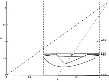
2.5 Equilibria for different values for k. 57

2.6 Equilibria for g = -0.2. 58

2.7 Equilibria for g = 0.2. 58

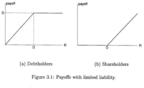
3.1 Payoffs with limited liability. 62

3.2

Separating

equilibrium.

k = 0.5,

A =

1 and

T =

[1,1.8].

78

3.3 Separating equilibrium. 78

3.4 Discrete pooling equilibrium. k = 0.5, A = 1 and T = [1,5]. 79

Acknowledgements

Ao orientador Aloisio Araújo, que fez de mim um doutor.

Ao co-autor Humberto Moreira, que me ensinou a resolver os proble

mas sem a propriedade do single-crossing.

A Walter Novaes, Heitor Almeida e Fábio Kanczuk pelos comentários

tão importantes para o futuro deste trabalho.

A Luis Braido, Daniel Ferreira, Paulo César Coimbra Lisboa e partici

pantes do workshop de microeconomia, no qual versões preliminares dos

capítulos da tese foram apresentadas e amadureceram.

A Samuel Pessoa, que me incentivou a fazer o doutorado nesta escola.

A Mônica

Viegas,

Joísa

Dutra,

Ricardo

Brito,

Márcia

Leon,

Ana

Lúcia

Vahia de Abreu e os muitos alunos que fizeram e fazem da EPGE uma

escola viva e de alta qualidade.

Aos professores da EPGE pelo contínuo estímulo intelectual.

Aos funcionários da EPGE, da Biblioteca Mário Henrique Simonsen

e da portaria da FGV, que, no dia-a-dia, tornaram agradável o meu tra

balho.

À CAPES

e à Fundação

Getulio

Vargas

o tão

necessário

apoio

finan

ceiro.

À minha

família

e aos

amigos

em

São

Paulo,

pela

paciência,

pelo

apoio

e pela compreensão.

Aos

muitos

amigos

que

fiz

no

Rio

de

Janeiro,

que

me

acolheram

e que,

desde os primeiros dias, me fizeram sentir em casa.

A todos

estes

que,

ao

longo

dos

quatro

anos

e meio

em

que

me

dediquei

ao

doutorado,

contribuíram

para

o sucesso

deste

projeto,

meus

sinceros

Essays

on

Asymmetric

Information

Problems

without

the

Single-Crossing

Property:

Introduction

Asymmetric .information plays an important role in a great number of situations

in corporate finance. Moral hazard, adverse selection and signaling models

produced many insights about how the economic players interact when some

information is not available to everyone. On the empirical side, researchers

test the implications of these models. Agency problems, information contents

of dividends, incentives in executive compensation, corporate governance, and

other concepts are, each one, large fields in corporate finance.

The objective of this dissertation is to re-examine classical issues in corpo

rate finance, applying a new analytical tool. The single-crossing property, also

called Spence-Mirrlees condition, is not required in the models developed here.

This property has been a standard assumption in adverse selection and signal

ing models developed so far. The classical papers by Guesnerie and Laffont

(1984) and Riley (1979) assume it. In the simplest case, for a consumer with

a privately known taste, the single-crossing property states that the marginal

utility of a good is monotone with respect to the taste. This assumption has

an important consequence to the result of the model: the relationship between

the private parameter and the quantity of the good assigned to the agent is

ordinary consumer, this property is frequently absent in the objective function

of the agents for more elaborate models. The lack of a characterization for the

non-single crossing context has hindered the exploration of models that

gener-ate objective functions without this property. The first work that characterizes

the optimal contract without the single-crossing property is Araújo and Moreira

(2001a) and, for the competitive case, Araújo and Moreira (2001b). The main

implication is that a partial separation of types may be observed. Two sets of

disconnected types of agents may choose the same contract, in adverse selection

problems, or signal with the same levei of signal, in signaling models.

In the three essays of this dissertation, three asymmetric information models

without the single-crossing property are developed. The first model examines

the trade-off between risk and incentives, which is a relevant issue in

execu-tive compensation literature. The traditional models of moral hazard imply a

negative relationship between risk and incentives, that is, when the owner of a

firm cannot observe the effort of the manager, the share of profits given to the

manager should be higher in riskier firms. This prediction is not supported by

the empirical work. In the model presented here, the manager is able to control

the mean and the variance of the profits. Additionally, the manager self-selects

his contract. In the resulting optimal contract, risk and incentives may have a

positive relation. Managers with higher risk aversion exert more effort in risk

reduction and selects contracts with lower incentives.

Signaling models provided many contributions to the corporate finance (see

Riley 2001). The determinants of corporate structure and dividend policy are

about the informational content of dividends. The traditional signaling models

assume the manager are better informed about the future prospects of the firm

and signal this knowledge using dividends. Empirical researches confirm the

prediction that the price of the shares and dividends are positively related.

However, a second prediction, the positive relationship between dividends and

earnings, is not empirically verified. In the signaling model presented here, a

correlation between current earnings and investment opportunities is introduced

and, in the resulting equilibrium, high-quality firms and low-quality firais can

signal with the same levei of dividends. Dividends and earnings may have an

ambiguous relationship, while, the relationship between prices and dividends

remains positive.

In the third model, a firm signals using debt. and the signal is observed by

the debt and stock markets. Although the separating equilibrium is possible,

partial separation equilibrium also arises. In this case, the two markets have

opposite interpretations about the signal. For the debt market, debt is a bad

signal, while, for the stock market, it is a good signal. The consequence from the

interaction of the two effects is that the benefit of the signaling is weaker. The

stock market is prone to give a good evaluation to the pool of firms that issues

debt, but the debt market demands a high discount. As the stock market takes

the debt market behavior into account, the value of the shares is reduced. As

is explained in the essay, the difference in the interpretations about the signal

is caused by the limited liability of the firm.

the traditional models does not hold without the single-crossing property. This

result has considerable consequences on the empirical work. Many tests are

based on the monotonic relationship implied by the traditional models, and an

insignificant correlation has been considered evidence that the information

is-sues has little importance in the situation analyzed. However, when the problem

does not have the single-crossing property, the asymmetry on the distribution

of information plays a role, even if the variables do not exhibit the monotonic

relationship.

The lack of a theory that characterizes contracts and equilibrium without

the single-crossing property has constrained the applied research. As this prop

erty may be naturally violated in economic problems, many relevant issues are

neglected by the current literature. The models presented here show that the

characterization in a more general context is tractable, insightful and changes

Chapter

1

Risk

and

incentives

with

multitask

Abstract

Standard models of moral hazard predict a negative relationship

be-tween risk and incentives, but the empirical work has not confirmed this

prediction. In this paper we propose a model with adverse selection

fol-lowed by moral hazard, where eífort and the degree of risk aversion are

private information of an agent who can control the mean and the

vari-ance of profits. As a consequence, the utility function of the agent may

not have the single-crossing property. In the resulting contract, the rela

tionship between risk aversion and incentives may not be monotone and

the relationship between incentives and observed variance of profits may

1.1

Introduction

Moral hazard plays a central role in problems involving delegation of tasks.

When the principal cannot perfectly observe the effort the agent exerts, the

payment must be designed taking into account the trade-off between incentives

and risk sharing.

Standard models of moral hazard predict a negative relationship between

risk and incentives. The central reference is the model presented in Holmstrom

and Milgrom (1987), that analyzes the conditions in which optimal contracts

are linear, that is, the agenfs payoff is a fixed part plus a proportion of profits.

In their model, the negative relationship between risk and incentives results

from the interaction between these two variables in the risk premium of the

agent. As the agent is risk averse and incentives put risk in agenfs payoff,

incentives incur a cost in utility. At the optimal incentive, an increase in risk

is balanced by a reduction in incentives.

The empirical work does not verify the negative relationship between risk

and incentives, and sometimes finds opposite results. Prendergast (2002) presents

a survey of empirical studies in three application fields, namely, executive

com-pensation, sharecropping and franchising. Positive or insignificant relationships

are found in the three fields and negative relationship is found only in studies

about executive compensation. The conclusion is that the evidence is weak.

Similarly, in the insurance literature, the monotone relationship between risk

and coverage is not verified as in Chiappori and Salanié (2000).

mod-eis, compatible with the observed facts. Prendergast (2002) suggests that in

centives are a substitute for monitoring in riskier projects, as monitoring is

harder in riskier environments. Ghatak and Pandey (2000) develop a model

with limited liability and moral hazard in effort and risk.

We propose a model with adverse selection, moral hazard and multitask.

Multitask models were first developed in Holmstrom and Milgrom (1991), but

in these models, effort controls exclusively the mean of the profits. In our

work, we consider the possibility of manager to control the variance of the

profits. Note that the observed variance is endogenous, and we can define

two types of risk: the exogenous risk is the intrinsic risk of the firm, and the

endogenous risk is the risk resulting from the effort of the agent in reducing

variance. Another feature in our model is the presence of adverse selection

before moral hazard. The principal does not know the risk aversion of the

agent and designs a menu of contracts so that self-selection reveals the type

of the agent. Sung (1995) shows that linear contracts are optimal in moral

hazard problem in which the agent controls risk. Sung (2002) shows that these

contracts are optimal in adverse selection with moral hazard, in a model with

more restrictive assumptions than the ours, and suggests that optimality is

valid in a more general setting. Although the optimality of liner contract is not

established for our model, we assume linearity and restrict the analysis to the

space of linear contracts.

In standard models, the agent cannot control the risk of the project and

However, when agents can exert effort in risk reduction, the direction of

selec-tion may change. An agent with high risk aversion may prefer a high incentive

contract, as he can reduce risk and the cost associated with risk. Technically

speaking, our model does not have the single-crossing property. Consequently,

the relationship between the incentives given to the agent and his risk aversion

is ambiguous. We computed the optimal contracts for representative situations

and found that the relationship between endogenous risk and incentives is am

biguous. For a set of agents with high risk aversion, incentives and observed risk

are negatively related. For a set of agents with low risk aversion, the relation

ship is positive. With respect to exogenous risk, the Holmstrom and Milgrom

result is preserved: the relationship between exogenous risk and incentives is

negative. In Araújo and Moreira (2001b), a model akin to the one presented

here is studied, applied to the insurance market.

In Section 1.2, we present the general model. In Section 1.3, we give two

examples. First, the single-task model is examined and the traditional relation

ship between risk and incentives is found. The multitask case is presented in

the second model. In Section 1.4, we compute the optimal contracts for

rele-vant cases of multitask model and we find positive and negative relationships.

Section 1.5 concludes. In Appendix l.A, we discuss implementability and

opti-mality without the single-crossing property, and, in Appendix l.B, we examine

the technical conditions for computing the optimal contract in the multitask

1.2

The

Model

The principal delegates the management of the firm to the agent, whose effort

can affect the probability distribution of the profits. Let e be the vector of

efforts

and

z be

the

profits,

with

normal

distribution

N (/j,(e),

a2 (e)).

Let

c(e)

denote the cost of the effort for the agent. The agent has exponential utility

with risk aversion 6 > 0, uniformly distributed on O = [6a,ôb\. At the time of

contracting, the agent knows his risk aversion, but the principal does not. We

will occasionally refer to 6 as the type of the agent. We assume the wage is a

linear function of the profits, that is, w = az + /?, 0 < a < 1. The contract

parameter a is the proportion of the profits received by the agent and is called

the incentive, or the power, of the contract. The parameter /? is the fixed part

of the contract which is adjusted in order to induce the agent to participate.

The timing of the problem is as follows: (1) the agent learns his type,

then

(2)

the

principal

offers

a menu

of contracts

{a(9),f3(9)}eee^

(3)

the agent

chooses a contract, and (4) exerts effort accordingly, (5) the firm produces profit

z and (6) the agent receives w az 4- f3 and the principal earns the net profit,

z w. The certainty equivalence of the agenfs utility is

a2

Vce((*,(3,9,e)

= f3 + a/i(e)

- c(e)

- 9o2{e),

that is, the expected wage, minus the cost of the effort and the risk premium.

The last term is the origin of the negative relationship between risk and incen

tives in purê moral hazard models. The risk premium acts as a cost because

the

principal

compensates

an

increase

of

o2

by

a reduction

of

a,

and

equates

the marginal cost and the marginal benefit of incentive. With adverse selection

preceding moral hazard, a similar effect exists: the principal has to compensate

the agent for the costs, in order to induce participation and truth-telling.

Let e*(a,9) denote the agent 0's optimal choice of effort, given a. Note that

e* is independent of (3. The resulting indirect utility is V(a,(3,9) f3 + v(a,6),

where

v(a,9)

= a/x(e>,0))

- c(e>,0))

- ±a29a2(e*(a,9)).

(I)

The problem is henceforth reduced to an adverse selection problem where

the agent has quasi-linear utility V(a,(3,6).

Assume the principal is risk-neutral. Her utility, given 9, is the expectation

of the net profit, that is, the profit after the wage is paid to the agent,

U(a,P,9)

= E[z

-w]

= (l-

a)/i(e>,0))

- 0,

where the expectation is taken with respect to the conditional distribution of

z, given the effort choice of the agent 9 under the contract (a, (3).

The adverse selection problem is to find the functions a(-) and /?() such

that

(<*(),/?()) G &Tgm3xE[U(a(9),P(9),9)} (2)

subject to

V(a(9),(3(9),8)

> V(a(ê),(3(9),9)M

ali 9,9

6,

(3)

)>O,forall0ee. (4)

The expectation in (2) is taken with respect to 9. The constraint (3) is the in

centive compatibility condition (IC). A function a(-) is called implementable, if

there is a function /?() that satisfies (IC). The constraint (4) is the participation

constraint (IR) where the reservation utility is normalized to be zero.

Guesnerie and Laffont (1984) fully characterize the optimal contract under

the assumption of single-crossing property, that is, the cross derivative vae has

constant sign. The solution of the model involves the definition of the virtual

surplus

f(a,9)

= M(e>,0))

- c(e*(a,0))

- i<*W(e>,0))

+ (9 - 9a)v9(a,9),

(5)

and the calculation of ai(0) = argmax/(<*,#). The optimal contract is a

combination of ai (9) and intervals of bunching.

In our model, the envelope theorem gives the marginal utility of incentive as

va(a,

9)

= /x(e*(a,

9))a9a2(e*(a,9)),

that

is,

the

mean

of the

profits

minus

the

marginal risk premium. As agents with higher risk aversion exert more effort in

risk reduction, the marginal risk premium term may increase or decrease with

agenfs risk aversion. Consequently, the cross derivative vag may have any sign.

The characterization of optimal contracts without the single-crossing property

is analyzed in Araújo and Moreira (2001a), and the Appendix l.A presents

some relevant results for the solution of our model.

1.3

Two

Examples:

Single-Task

and

Multitask

are under control of the agent. In the multitask case, the observed risk is

endogenous.

1.3.1 Single-Task

We first analyze the single-task specification where agenfs effort controls only

the mean of the profits. Let eM denote the effort and assume the mean of

the profits is linear in eM, /x(eM) = /xeM, and the cost of effort is quadratic,

c(e^)

= e2/2.

The

certainty

equivalence

is

Vce

=

P-The agent chooses e£ = a/z and the resulting indirect utility is V(a,(3,9) =

(3 + v(a,9), where

The

marginal

utility

of incentive

is va

= ctfi2

a.9a2.

An

increase

in incentives

has positive and negative effects on the utility of the agent. The positive effect

is the increase of the share of profits. The negative effect comes from the

increase of risk in the wage. The single-crossing property holds for this case,

since

vag

=

aa2

< 0.

An

agent

with

low

risk

aversion

has

high marginal

utility of incentive and may select a contract with high degree of incentives.

The

virtual

surplus

is /(a,

9) = a/x2

^a2/x2

\a29a2

+ (9

9a)vg

and

the

solution of the relaxed problem is given by the first-order condition fa(a, 9) 0,

that is,

«w

=

The function a is decreasing in 6 and va$ is negative, therefore, the relaxed

solution

is the

optimal

contract

of the

original

problem.

The

variance

a2 has

also a negative effect on a, due to the two last terms in the virtual surplus, that

is, it increases the marginal cost from risk premium and informational rent.

The

relationship

between

a and

o2

is still

negative,

given

6.

Therefore,

adverse selection before moral hazard is not sufficient to change the traditional

risk-incentive trade-off. If agent controls only the mean of the profits, risk does

not affect the benefit of principal, because she is risk neutral, but increases the

marginal cost, because she has to compensate for the risk premium and has to

pay the informational rent. Consequently, the incentive offered is lower.

1.3.2 Multitask

We introduce the possibility for the agent to control the variance of the profits.

Let e^ and ea be the effort exerted in mean increase and in variance reduction,

respectively.

Let

fi(e)

= \xe^

cr2(e)

= (oq

ea)2

and

c(e)

\{e2L

+ e2,),

where

<7o is the exogenous variance. The certainty equivalence is

The optimal choices of effort are

e = afj., and ea = 9 a0 < a0.

The effort in mean, e^ is higher, the higher is the incentive. The effort in

variance reduction, ea, is higher, the higher is the incentive, the risk aversion

and

the

exogenous

variance

of

the

pronts.

The

observed

variance,

<r2(e*)

=

The envelope theorem gives the derivatives

va = /ieM

- aé>(<70

~ ea)2,

a2

.

.,

ve = -y(ffo-e<7)

< 0.

The first derivative states that the utility increases with a, due to the mean of

the profits, but decreases, due to the risk premium.

And the cross-derivative is

= fJ--^-

~ "(co

- eCT)2

+ 2a0(ero

-

ea)-^-=o <o >o

The first term is zero, that is, the marginal utility is not affected by the effort

in the mean of the profits. The other two terms derive from risk premium.

The

direct

effect,

a(<7o

eCT)2,

has

an

interpretation

similar

to the

single-task

case, the higher is the risk aversion, the higher is the effect of incentive in risk

premium.

The

effect

via

effort

is 2a6(ao

ea)^f-

and

acts

in opposite

direction.

Marginal utility increases with 0 because high risk-aversion agent exert more

effort in risk reduction. In our example,

and the function ao(9) = \/\/6 defines a decreasing border between vag > 0

and vag < 0 regions, with vag > 0, for a > ao- For low risk aversion agents, the

direct effect dominates and marginal utility of incentive decreases with type.

For high risk aversion agents, the effort has a opposite effect and the second

term dominates and vag > 0. This changes the self-selection direction, that is,

agent with a high type has a high marginal utility and chooses contracts with

more incentive.

The following expression is the virtual surplus of the problem,

2

The derivative with respect to a is

- a2ea)

+ (e-<

and the relaxed solution a\(9) is given by fa(cti(6),6) = 0 and /aa(<*i(#),#) <

0. Note that fa{0,6) > 0 and fa(l,õ) < 0, so relaxed problem has an interior

solution

and

fa(-,0)

has

at

least

one

root

in

the

interval

[0,1].

If /(-,#)

is not

concave in a, the incentive that maximizes the virtual surplus must be correctly

chosen among solutions of the first order condition.

The solution of the relaxed problem is the optimal contract if the incen

tive compatibility constraint is satisfied. As single-crossing does not hold, the

incentive compatibility is not obvious and, when ai(6) is not implementable,

the computation of optimal contract must follow the procedure presented in

Appendix l.A.

When vag(ai(6),6) is positive and negative, the optimal contract must

con-sider the possibility of discrete pooling. When 6 and 0 are discretely pooled,

the conjugation rule for the pooled types is

The discrete pooling segment, au(6), is given by the equation

(1 - a)(l

+ 0a2)2(l

+ 62aA)

= 2B2o?°\

A*

in Araújo and Moreira (2001a), as explained in Appendix l.B. The optimal

contract may have a complex form, that results from a combination of ai(9),

au(9) and bunching.

For a given ao, /x and [9a,9b], we compute the optimal contract a*(9) and

the

endogenous

risk

a2(e*(a*(9),9)),

and

plot

the

risk-incentive

curve

a x a2.

With respect to the endogenous risk, note that

2

When vaQ > 0, a(#) is increasing and risk is decreasing in 9. Consequently, risk

and incentives are negatively related. When vag < 0, a(9) is decreasing and

risk

and

incentives

may

be

positively

related

if 9a2

(9)

is increasing

in

9.

That

is, the endogenous risk decreases with risk aversion, provided that a(9) does

not decrease too fast.

1.4

Results

The equations above for the multitask example were numerically implemented

for the three cases listed in Appendix l.B. The parameter values, <xo = 0.91

and fi = 1, are the same for the three cases, and the values of 9a and 6f,

change. In Figure 1.1, for 9 [2.5,3.5], the relaxed solution is increasing, and

coincides with the optimal contract. Figure 1.2 is the corresponding plot for

risk and incentives. An agent with higher risk aversion chooses higher incentive

contracts, because he reduces the marginal cost from risk premium by exerting

more effort in risk reduction. The relationship between risk and incentive is

negative as in Holmstrom and Milgrom.

The contract for a set of types with lower risk aversion, 9 [0.5,1.4], is

shown in Figure 1.3. The relaxed solution is implementable as vae(ot\(6a),6b) <

0. The optimal contract coincides with the relaxed solution, but this time

the relationship is reversed. The higher types have higher marginal cost of

incentives, thus they prefer the lower incentive contracts. At the same time,

more risk-averse agents exert more effort in risk reduction and the variance is

lower. As is seen in Figure 1.4, the risk and incentives are positively related.

For a broader interval of types, that encompasses vag of both signs, the

discrete pooling is possible and the optimal contract presents a U-shaped form.

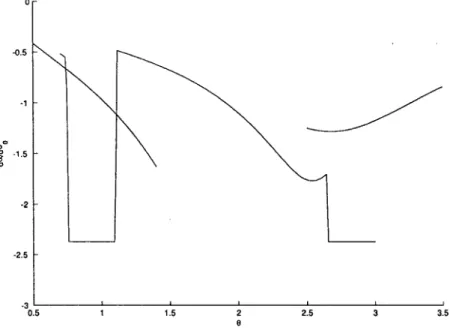
In Figure 1.5, the optimal contract for 6 [0.7,3.0] is plotted. As prescribed in

Appendix l.B, the validity of assumptions A2 and A3 were checked numerically.

Computational procedures found the optimal contract that combines ai, au and

bunching. Incentives and risk aversion are positively related in a higher risk

aversions subset and negatively related in a lower risk aversion subset. The

U-shape of the optimal contract is also present in risk-incentive graph, as we

can see in Figure 1.6.

The results above are concerned to the endogenous risk. The relationship

between exogenous risk and incentives was numerically calculated for the three

cases above. As shown in Figure 1.7, the sensitivity da/dao is negative, that

1.5

Conclusion

The negative relationship between risk and incentives is not preserved if the

agent can control the variance. A higher risk aversion agent exerts more effort

in reduction of risk. The relationship between risk and incentives is positive

if more risk averse agents select low powered contracts. This is true when the

marginal utility of incentive is decreasing with risk aversion. However, if risk

aversion is high enough, the possibility of risk reduction may reverse this effect

and the traditional negative relationship between risk and incentives may be

observed. The optimal contract may also be U-shaped, such that, agents with

intermediate risk aversion choose contracts with low incentives, and agents with

extremely high or extremely low risk aversion choose high-incentive contracts.

The numerical calculations suggest that the relationship between incentives and

exogenous risk remains negative.

Apendix

l.A

l.A

Adverse

Selection

without

the

Single-Crossing

Property

We report below the main results from optimal contract in non-single-crossing

context. Most of results are in Araújo and Moreira (2001a).

l.A.l Incentive Compatibility and Participation Constraint

When a(-) and /?() are differentiable, the incentive compatibility may be locally

checked by the first and second order conditions. These conditions are necessary

but not sufficient for incentive compatibility. The íirst order condition gives

va(a(e),e)a'(6)+l3'(e) = 0, (7)

which states that indiíference curves of type 0 agent must be tangent to an

implementable contract on a x f3 plane, at point (a(6), f3(0)).

The second order condition gives

vaa(a(9),e)[a'(e)]2

+ va(a(e),e)a"(e)

+ (3"(e)

< o,

(8)

and, after diíferentiating (7) with respect to 6, the expression (8) simplifies to

the condition

va9(a(8),e)a'(e)>0,

(9)

which implies the monotonicity of a(6), in the single-crossing context.

Define the informational rent of the agent 9, r(6), as the levei of utility

achieved by this agent, given the menu of implementable contracts (a(#),/?(#)),

that is, r(9) = v(a{0),0) +/?(#). Using (7), we get

r'(0) = ve(a(e),6), (10)

and

applying

the

envelope

theorem

on

(1),

we

have

ve(a,9)

= ^a2a2(e*)

<

informational

rent.

Thus,

the

participation

constraint

is active

for

the

highest

type, 6b, that is, r(6b) = 0.

The

fixed

component

of

the

wage

can

be

isolated

by

integration

of

r'(6),

ve(a(0),

ê)dÕ

- v(a(0),

6).

(11)

1.A.2

Implementability

without

the

Single-Crossing

Property

Since

the

single-crossing

property

is not

ensured,

the

first

and

the

second

order

condition are necessary but they are not sufncient. The following points must

be observed:

1. The function a(6) may be non-monotone. The same contract may be

chosen by a discrete set of agents. We call this situation as discrete

pooling. In this case, the pooled types follow the conjugation rule

va(a(e),e)

= va(a(e'),e'),

(12)

whenever a(6) = a(6'), which states that the indifference curves of 6 and

& are

both

tangent

to

the

menu

of contracts

on

a x (3 plane.

2. The incentive compatibility must be globally checked. When the

single-crossing property holds, the incentive compatibility may be only checked

locally. If types in the neighborhood of 6 is not better with the con

tract assigned to 6, no other type will be better. The first and second

order conditions are sufncient for global incentive compatibility. On the

other hand, if the single-crossing property is violated, types out of the

neighborhood of 6 may prefer the contract assigned to 9.

20

BIBLIOTECA

MÁRIO

HENRIQUE

SIMONSEN

-3. The function a(9) may be discontinuous. The possibility of discrete

pool-ing creates jumps in the optimal assignment of contracts, so we allow the

contract to be piecewise continuous. More precisely, we assume that the

functions are right continuous with limit from the left. When jump occurs,

the agent must be indifferent between the start and the end point of the

jump. For example, if there is a jump in 9 and agent 9 were strictly better

with the end point than the start point, then, for a small e > 0, the agents

with type in [9 - e, 9) would strictly prefer the end point, contradicting

the initial assumption of jump in 9.

1.A.3

Virtual

Surplus

and

the

Principal's

Problem

We

follow

the

standard

procedure

and

define

the

social

and

virtual

surplus,

S{a,9)

= /x(e>,0))

- c(e>,0))

- ^aW(e>,0)),

(13)

f(a,9)

= S(a,

9)+

{9-

6a)vg(a,

9).

(14)

The

expression

(13)

defines

the

social

surplus

S(a,6).

The

maximization

of

social

surplus

for

each

9 gives

the

first

best

of

the

model.

The

virtual

surplus,

defined in (14), is the social surplus plus the informational rent term. This term

is negative

and

represents

a cost

that

takes

into

account

the

rent

that

is paid

to

the agents

with

risk

aversion

in

[9a,

9],

in order

to

preserve

implementability

when agent 9 receives a(9).

Let p(0) and P{9) be the probability density and the cumulative of 9. The

expectation of integral term may be simplified by Fubini's theorem as,

where

^/

= 9

9a,

for

the

uniform

distribution.

Then,

the

principal's

objective

function

can

be

written

as

E[f(a(9),6)].

After the optimal incentive, a*(6), is found, the fixed part of optimal contract,

(3*(9), can be calculated using (11).

The maximizatiom problem of principal without the constraints is called

relaxed problem. Its solution, denoted a\(9), satisfies

fQ(a1{9),9) = 0 and faa(oti{9),9) < 0.

Since /a(ai(0),0) = Sa(ai(9),9) + (9- 9a)va6(ai(9),9), the relaxed solution

provides less incentive than the flrst best when vae < 0, and more incentive

when

vae

> 0.

This

distortion

occurs

because

the

cross

derivative

is associated

with

the

marginal

cost

of

informational

rent.

For

example,

when

vae

< 0,

the

cost of

informational

rent

is increasing

with

respect

to a,

therefore

the

principal

pays less incentive.

1.A.4

Optimality

without

the

Single-Crossing

Property

In the standard adverse selection model, the single-crossing property ensures

that

a\(9)

is the

optimal

contract

if (9)

is satisfied,

that

is,

a\(9)

is

non-increasing

when

vae

<

0,

or

non-decreasing

when

vae

>

0.

When

(9)

does

not

hold,

the

optimal

contract

is the

best

combination

of ol\{9)

and

intervals

of

bunching so that (9) is satisfied. That procedure is not suitable in the absence

of the single-crossing property. As before, a\{9) is the optimal contract if it is

implementable. However, monotonicity condition (9) is no more sufficient for

implementability and global incentive condition must be checked.

Moreover, when vag change its sign, the discrete pooling is possible and

ot\{Q) is not the optimal contract for the pooled types. The assignment of

contracts to the discretely pooled types must take into account the conjugation

of types according to the constraint (12). Let au(6) denote the assignment of

contracts in a discrete pooling. Then

'), (15)

fa(ç*u(e),e) = fa(au(e'),e>)

The optimal contract will be a combination of a\(9), bunching and au(6). We

follow Araújo and Moreira (2001a) and restrict the solution a* (6) to the closure

of the continuous functions. The optimal contract with discrete pooling can be

characterized under the following assumptions:

Al. vag(a,9) = 0 defines a decreasing function ao(9), vag is positive above

and negative below ao(9), for ali 9 ©.

A2. ai

is U-shaped,

crosses

ao

in

an

increasing

way,

ot\(9a)

< ai(0b),

fa(&,9)

is negative above and positive below a\(9), for ali 9 G 0.

A3. For each 9, the equations va{a\(),) = va(ai(-),9) have at most one

solution in the decreasing part of ai, on vae < 0 region.

Under these assumptions, the optimal contract, a*(9), will have one of the

following forms:

a* (9) =

au(9), i£9<9u

), ií9>9u

where 9\ is defined by otu(9\) = au(9a), or

<*(*)

=

min{ã,au(9)}, ií9>92,

where ã is the incentive of the bunching and 92 is defined by ai (#2) = ã. The

set of bunched types, J = {9 G 9 : a(#) = ã}, satisfies

[ fa(ã,9)p(9)d9

= 0.

J

Apendix

l.B

l.B

Optimal

Contract

in

the

Multitask

Specification

As in the single-crossing case, the solution of relaxed problem, ac\(9), is the

optimal contract if it is implementable. However, condition (9) is not sufficient

for implementability.

The following definition will be useful for global analysis of incentive

com-patibility. For a given contract a(9) define the integral $(9,9) as

rê

rÔ f rctiê)

$(9,9)

= /

/

va6(ã,9)ò

Je Jate)

dê.

(19)

It can be shown, using (10), that $(6,6) = V(a(9),@(6),9) - V(a(9),(3(9),9),

thus $(9,9) is the difference for agent 9 between the utility of the contract

assigned to himself and the one assigned to 9. The (IC) constraint can be

stated as

$(9,9)

>0,

forallfl.êee,

that is, the agent with risk aversion 6 is not better pretending to be an agent

with risk aversion 6.

The numerical examples presented in Section 1.4 correspond to three cases

for which we can characterize the optimal contract.

(a) ai(9) is increasing and vag(ai(0),6) > 0.

Since ao(O) is decreasing, the region of integration in (19) is in vag > 0

region. Therefore $(9,6) > 0 and c*i(0) is the optimal contract.

(b) ai(0) is decreasing and vag(ai(6),6) < 0.

A sufficient

condition

for

implementability

is vae(ot\(6a),0b)

< 0-

As

ao(6)

is a decreasing

function,

the

region

if integration

in (19)

is in

vag

<

0

region. Then ${0,6) > 0 and c*i(0) is the optimal contract.

(c) vae(ai(6),e) has any sign.

In this case, the optimal contract can be computed by the procedure in

Appendix l.A, if assumptions Al, A2 and A3 hold. Assumption Al holds

since,

from

equation

(6),

the

function

ao(6)

= l/y/ô

defines

a decreasing

border between vag > 0 and vag < 0 regions, with vaQ > 0, for a > a0.

The following proposition shows that the first part of assumption A2

holds.

Proposition 1 Let 9X be defined byot\(6x) = ao(9x). If6x exists, a'x(^x) >

0.

function theorem,

>(0\-

f

ai{9)

~ -f

and, as second order condition states that faa(&i(9),9) < 0, a'i(9) has

the same sign as fao{oi\{9),9). Differentiating fa with respect to 9,

') =

and manipulating this expression, we conclude that a[(9) has the same

sign as

On

ao(e),a

=

1/y/Õ.

Then,

h(ao(ex),ex)

= 0X(1

- 0a/6x)(2

+ 6a/6x)t

which

is positive

for

6X

> 9a-

Therefore

a'x{9x)

> 0.

However, the second part of A2, and A3 is not valid for every value of

parameters and must be checked before the application of the procedure

in Appendix l.A.

1

0.95

0.9

0.85

0.8

0.75

0.7

0.65

\ \

XÁ

'.

0 0.5 1 1.5 2 25 3 3.5 4

Figure

1.1:

Optimal

contract.

<r0

= 0.91,

\i = 1 and

0 = [2.5,3.5].

0.85

0.7

0.1 0.15

1

0.95

0.9

0.85

O.S

0.75

0.7

0.65

0.6

' \

-\

\ "o

\

i i i i

^

O 0.2 0.4 0.6 0.8 1 1.2 1.4 1.6 1.8

Figure 1.3: Optimal contract. oç> = 0.91, /x = 1 and © = [0.5,1.4].

0.2 0.3 0.4 0.5 0.6 0.7

Figure 1.4: Risk x incentives, <jq = 0.91, \i = 1 and 6 = [0.5,1.4].

0.75

0.65

1.5

Figure

1.5:

Optimal

contract.

oQ

= 0.91,

/x = 1 and

G = [0.7,3.0].

_i 1

0.05 0.1 0.15 02 025 0.3 0.35 0.4 0.45 0.5

Figure 1.7: Exogenous risk x incentives.

Chapter

2

Do

dividends

signal

more

earnings?

Abstract

Signaling models have contributed to the corporate finance literature

by formalizing "the informational content of dividends" hypothesis.

How-ever, these models are under criticism of empirical literature, as weak

evidences were found supporting one of the main predictions: the positive

relation between changes in dividends and changes in earnings. We claim

that the failure to verify this prediction does not invalidate the signaling

approach. The models developed up to now assume or derive utility

func-tions with the single-crossing property. We show that signaling is possible

in the absence of this property and, in this case, changes in dividend and

2.1

Introduction

The information content of dividends is a controversial issue in corporate

fi-nance. The research started when Miller and Modigliani (1961) suggested that

managers use dividend policy to convey their expectations of future prospects

of the firm. With this hypothesis they proposed to explain the effect of div

idend changes on the prices of shares. Since then. theoretical and empirical

research advanced. Signaling models were the main tool that formalized the

original intuition. Bhattacharya (1979), Miller and Rock (1985), and John and

Williams

(1985)

were

the

initiators

of a long

list

of signaling

models1.

The

basic

idea is that firm managers possess private information about future earnings

and they like to convey it to the market. However, they cannot simply announce

their expectations of future earnings publicly because every firm could imitate

them. The information is conveyed by a costly signal. In the cited models,

the respective costs are: financing of a committed levei of dividend, suboptimal

investment and tax on dividends.

On the empirical side, researchers tries to verify the testable implications

derived from the models. In ali these models the single-crossing property holds.

As a consequence, the models predict that dividends, market price and future

or current earnings are positively related. The correlation between dividend

and returns was a strongly established result even before the signaling models

have appeared. Aharony and Swary (1980) show that announcements of

divi-'See AUen and Michaely (1995) for a survey on theoretical and empirical issues on dividend

policy.

dend increases or decreases result in, respectively, positive or negative abnormal

returns.

The controversy lays on the relationship between dividends and subsequent

earnings. Watts (1973) analysis found the positive relation, however, the effect

was very small and not conclusive. Healy and Palepu (1988) found a

signif-icant relation, but they focused in the particular situation of initiation and

omission of dividend payment. Exploring a larger data set Benartzi, Michaely

and Thaler (1997) found no significant relation between dividends and future

earnings and concluded that dividends are more related to past and present

earnings. More recently, Nissim and Ziv (2001) using an improved measure of

future earnings concluded that dividends matters for earnings prediction. Many

other works contributed to this debate and a definitive conclusion seems far to

be reached.

We claim that the lack of a clear relation between dividends and earnings

is not incompatible with information content of dividends. Common to ali the

previous models of signaling is the existence of single-crossing in the objective

function of manager, i.e., the marginal cost of signaling is monotonic in the

type of firms. This property generates the monotonic relationship between

dividends and earnings. In this work, we drop this assumption and develop

a model employing the techniques presented in Araújo and Moreira (2001a).

In non-single-crossing signaling, a new kind of equilibrium may exist. In this

equilibrium the relation between firms earnings and dividends is U-shaped, so

types pretending to be high types. The market value of shares is an average of

the values of two types and increases with dividend. So, signaling models may

provide a positive relation between dividends and market price and, at same

time, an ambiguous relation between dividends and earnings.

The model is presented in Section 2.2 and it is similar to the model of Miller

and Rock (1985). For concreteness, we assume a quadratic production function,

in Section 2.3, and discuss an example. Computations are performed for a range

of parameters values and results are presented in Section 2.4. We comment the

connections with the empirical literature in Section 2.5. The conclusions are

presented in Section 2.6.

2.2

The

Model

This model builds on Miller and Rock (1985). There is a firm with production

function F(-). The usual properties, F'(-) > 0 and F"(-) < 0, are assumed. Let

X and Y be the earnings, respectively, at period 1 and 2. At the beginning

of period 1, managers know X and announce dividends, D. Then shareholders

may sell their shares, dividends are distributed and X D are invested. At the

end of period 1, the firm production is subject to a multiplicative shock, 6 > 0,

so that

Y = 6F(X - D),

where 0 < D < X. At period 2 the earnings are distributed and the firm is

disassembled. We assume the firm cannot issue debt and investments have to

be financed exclusively by internai resources. The information asymmetry is on

the

knowledge

of X,

which

we

assume

randomly

distributed

on

[Xi,.?^],

with

density p(X). Consistent with the terminology used in theory of contracts,

we

refer

to

X

as

the

type of

the

firm.

At

period

1, managers

know

X

before

the dividend announcement, but the market does not, and managers cannot

credibly

convey

their

private

information

to the

market.

The

shock

8 is unknown

to both manager and market, but may be correlated with X.

Both

X

and

8 affect

the

value

of firm.

Now

suppose

the

manager

has

an

estimate

of

5 based

on

private

information

in

period

1.

If managers

are

inter-ested

on

market

value

of firm,

they

would

like

to sign

X

and

8 when

the

implied

value

is high.

The

signaling

of

X

is clear.

If a firm

pays

more

dividends,

it

incurs

in increasing

costs

due

to

underinvestment.

Since

higher

type

firms

have

higher

earnings,

their

sacrifice

in output

is lower

for

the

same

levei

of dividend.

The

decreasing

cost

of

dividend

allows

signaling

in

a way

that

higher

types

signal

with

higher

dividends.

Also,

they

would

like

to

reveal

8 to

the

market

but,

in

this

case,

the

signaling

is not

possible.

They

cannot

signal

high

pro-ductivity

distributing

more

dividends,

as

high

8 firms

has

higher

marginal

cost

of

dividend

because

optimal

investment

levei

is higher

and

sacrifice

in

output

is higher.

On

the

other

side,

a high

8 firm

cannot

signal

higher

investment

opportunity

paying

less

dividends

because

low

8 firms

could

imitate

paying

low

dividends.

However,

we

will

show

that

if X

and

8 are

correlated,

the

shock

in

productivity

may

produce

a signaling

in

which,

for

a subset

of

firms,

dividend

Assumption 1 The shocks are correlated,

E[6\X] = e(X) > 0.

2.2.1 The Value of the Firm

At period 1, managers estimate the fundamental cum-dividend value of the firm

as the present value of dividend flow:

V(X,

D) = D + ^-

E[8F{X

- D)\X]

^D).

(1)

Under symmetric information, this would be the value of shares and the

manager would choose the investment in order to maximize V. The first-best

dividend levei, D*, would be given by the Kuhn-Tucker conditions:

= 0, if D* > 0,

F'(X - D*)

-e(X)

(2)

> 0, if D* = 0.

But under asymmetric information, the market value may not coincide with

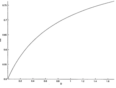
V. Let Vm denote the market value. We will assume that Vm is determined as

a signaling equilibrium, that is, firms signal to the market by the choice of div

idend levei and market estimates the value observing the dividend choice. The

firms will choose dividend above the optimal levei, paying an underinvestment

cost for signaling.

Shareholders want to maximize V if they keep the share with them until

period 2. The ones who intend to sell at period 1 prefer the maximization of the

market value, Vm. As in Miller and Rock (1985), we assume the firm's managers

are maximizing a welfare function that aggregates the interests of shareholders

that

desire

to

sell

the

shares

and

the

ones

who

do

not.

Let

k

(0,1]

be

the

fraction of shareholders that sell at period 1. This fraction is exogenous and can

be motivated by necessity of liquidity by shareholders. The welfare function is

W(X, D, Vm) = kVm + (1 - k)V(X, D).

For the purpose of signaling analysis, we are interested on marginal rate of

substitution between Vm and D. Since W is quasi-linear with respect to Vm,

ali the properties are found in marginal welfare of D,

W

D(X,

D) = (l-

k) (l -

-^-The dependence of productivity shock on type may make Wq non-monotone

on

type.

More

precisely,

higher

X

increases

e,

but

reduces

F',

for

the

same

levei of dividend.

In terms of the cross-derivative of W,

WXD(X,

D) = \^

[s(X)F"(X

-D)-

e'(X)F'(X

- D)]

,

(3)

may

change

its

sign.

We

can

define

two

regions

in

X

x D

plane,

according

to

this sign.

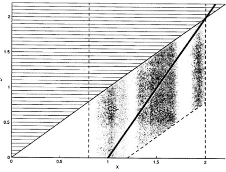
Definition 1 The CS+ region (resp. CS- region) is the set ofpoints inXxD

plane

such

that

Wxd

> 0 (resp.

Wxd

< 0).

In equation (3), the first term in the brackets is the investment effect. Firms

with higher earnings invest more and have lower marginal product.

Conse-quently, the marginal cost of dividend is lower for higher types. The second

Negative correlation between earnings and productivity

When e'(X) < 0, higher earnings reduce the expected productivity and the

cost of signaling is lower. Welfare function has the single-crossing property

since both productivity and investment effects collaborate on Wxd > 0. The

results are, therefore, similar to the ones found by Miller and Rock (1985).

Positive correlation between earnings and productivity

If e'(X) > 0, higher earnings correspond to a higher optimal investment levei

and dividend becomes costlier since more earnings should be retained for in

vestment. If, for some types and dividend levei, productivity effect dominates,

then Wxd < 0 and higher types will be more reluctant to pay dividends

be-cause of lost of investment opportunities. Conversely, Wxd > 0 holds when

investment effect dominates. In this case, lower types are more reluctant to pay

dividends because they have lesser investment resources. Note that from (2)

the first-best dividend as a function of types, D*(X), is increasing for Wxd > 0

and decreasing for Wxd < 0. If investment effect dominates, firms with higher

earnings may pay more dividends and, if productivity effect dominates, they

should invest more paying less dividends. When e'{X) > 0 is such that the

signal of Wxd is ambiguous, the single-crossing propriety does not hold. The

assumption on the constancy of sign (for instance in Riley (1979)) for

cross-derivative of objective function is then violated and we need another approach

developed in Araújo and Moreira (2001a,b).

An alternative setting, without the multiplicative shock, would be to assume

that the production function has increasing returns for low leveis of investment

and

decreasing

returns

otherwise.

In this

case,

Wxd

= \^F"{X

D)

and,

consequently, marginal cost of dividend increases with earnings only for firms

in increasing returns.

2.2.2 The Signaling Equilibrium

As usual, the signaling equilibrium is a perfect Bayesian one (the formal

de-finition is provided in appendix 2.A.1). The basic description remains. The

market generates a value function, Vm(-), and each type of firm, X, chooses a

dividend levei, D, that maximizes W. We have an equilibrium if zero expected

profit condition holds, that is,

Vm(D)

= Eli[V(X,D)\D],

(4)

where EM denotes the expectation taken on the Bayesian updated distribution

on X. The market value Vm should be the expected value of the firm with

respect to the probability distribution of X, resulting from the Bayesian update

given the choice of D by the firm.

Formally, the signaling problem consists in finding functions VTn{X) and

V{X) such that the type X firm chooses a dividend levei V{X) and is evaluated

as Vm(X)

by

the

market.

Since

dividends

and

market

value

are

linked

by

Vm(-),

these functions are related by Vm(X) = Vm{V{X)).

Define the welfare of type X firm that declares to be type X as

W(X,X) = W(X,V(X),Vm(V(X)))

In order to be incentive compatible, each firm should prefer to tell the truth,

that is

W(X,X)>W(X,X), (5)

for ali X,X G [Xi,^]. A differential equation for V is derived from the first

order condition

^X,X)

= 0.

(6)

It should be noted that the first order condition is not sufncient condition

for implementability when single-crossing property does not hold. Incentive

compatibility should be checked globally after a candidate for equilibrium is

obtained.

Additionally, the second order condition constrains V(X):

Proposition 1 In signaling equiHbrium, T>(X) is non-decreasing in CS+

re-gion and non-increasing in CS region.

Proof: See the appendix.

When single-crossing property is present, CS+ and CS do not show up

simultaneously and contracts should be monotone. As a consequence, types are

separated when V(X) ^ 0, or a interval of types is bunched when V{X) = 0.

When single-crossing property does not hold, monotonicity is not assured and

the relationship between type and signal may be, for example, U-shaped and a

disconnected set of types may signal with the same dividend levei.

2.2.3 Equilibria Diversity

In a equilibrium, the same signal, D, may be chosen by many types. We are

interested in classifying the equilibrium according to its degree of separability.

The following definition will be useful:

Definition 2 The pooling set, Q(D), is the set of types whose signal is D, that

In particular, in a separating equilibrium, Q(D) is singleton for every D

that is chosen by a firm.

Definition 3 The type X is separated ifQ(V(X)) {X}. A separating equi

librium is a signaling equilibrium such that every X is separated.

When X is separated, market correctly infers the type by the observation

of D. So Vm{D) = V(X,D), where X is the type that choose dividend levei

D.

Proposition 2 In an interval of separated types, V(X) follows the differential

equaüon

vD(x,v(x))

(7)

Proof: See the appendix.

As in the single-crossing case, a pooling equilibrium may be characterized

by a continuum of types that chooses the same signal levei.

Definition 4 The type X is continuously pooled, if QÇD(X)) is a continuous

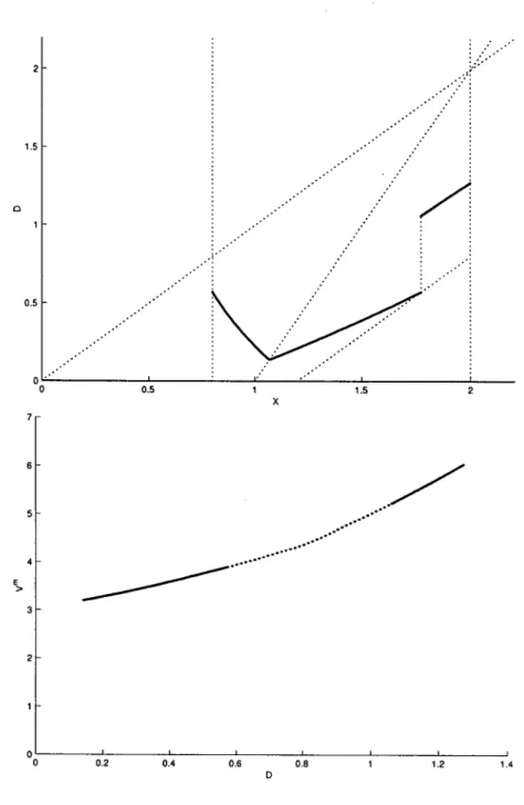
In signaling games without single-crossing condition, a new kind of pooling

arises. As in the continuous pooling, some values of D will be chosen by more

than one type of firm. However, the number of pooling types may be finite.

Definition 5 The type X is discretely pooled, if Q(V(X)) is a discrete and

finite set.

The property aggregating the discretely pooled types is that they must have

the same marginal welfare

Proposition

3 IfXa

and

Xb

are

discretely

pooled

and

D = V{Xa)

= V{Xb)

^

0, then

WD(Xa,D)

= WD{Xb,D).

(8)

Proof: See the appendix.

Equation (8) gives e(Xa)F'(Xa - D) = e(Xb)F'(Xb - D). So different

types can choose the same levei of dividend when, for higher types, the higher

productivity shock compensates the reduction in marginal productivity resulted

from higher investment. In the discrete pooling, dividend choice does not fully

reveal the type of the firm. The market knows the set of possible types but

it cannot distinguish one type from the other. This fact is taken into account

when the market estimates the value, so EM[V(X,D)|D] is the average value of

types in the pool.

Assumption 2 The type X is uniformly distributed on the interval [X

With Assumption 2, each type has the same probability. In particular, when

there are only two types in the pool, the expected value of firms is

E»\y(X,D)\D]

= \v{Xa,D)

+ \v{Xb,D),

where Xa and Xb are the types that choose D.

Proposition 4 Under Assumption 2, in a interval with discretely pooled types,

if exactly two types chooses the same dividend, T>(X) follows the differential

equation

v

WX(X(X,V),V)XD(X,V)

where X(X,D), derived from (8), is the type pooled together with type X, when

dividend D is chosen.

Proof: See the appendix.

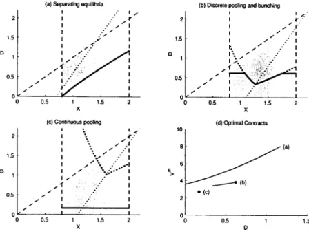
2.2.4 Equilibrium Refinement

The disturbing fact in any signaling model is the existence of many equilibria.

For the same parameters, different kinds of equilibrium may exist, and the

choice of initial conditions may generate a continuum of equilibria. At this point

a selection criterion is needed. The pro-separation equilibrium, defined below,

choose, among different kinds of equilibria, the one that minimizes pooling and

maximizes efHciency.

Assumption 3 Separability degree of a continuous pooled type, a discretely

Therefore 11(1) is the set of continuously pooled types, 11(2) is the set of

discretely pooled types and 11(3) is the set of separated types.

Definition 7 The separation floor of a signaling equilibrium is the lowest

sep-arability degree associated to a type in

[X\,X2]-Definition 8 A proseparation equilibrium is a signaling equilibrium with

sepa-rating floor cp, such that (a) there is no other equilibrium with higher separation

floor; (b) among equilibria with same separation floor, there is no other with

lower probability ofH((p), according to density p(-); and (c) among equilibria

with same separation floor and same probability ofH(ip), there is no other equi

libria with higher expected value, according to density p(-).

Therefore, pro-separation equilibrium criterion chooses an equilibrium

elim-inating poorly separated equilibria and taking the most efficient among the

surviving equilibria.

2.3

The

Quadratic

Case

For the computations we consider a quadratic production function

I), (10)

where 0 < I < 6/2, a > 0, and b > 0. We assume a linear expected productivity

shock

e(X)=g + hX, (11)

where h > 0.