www.hydrol-earth-syst-sci.net/18/4733/2014/ doi:10.5194/hess-18-4733-2014
© Author(s) 2014. CC Attribution 3.0 License.
Results from a full coupling of the HIRHAM regional climate model
and the MIKE SHE hydrological model for a Danish catchment
M. A. D. Larsen1,*, J. C. Refsgaard2, M. Drews3, M. B. Butts4, K. H. Jensen1, J. H. Christensen5, and O. B. Christensen5
1Department of Geosciences and Natural Resource Management, University of Copenhagen, Øster Voldgade 10,
1350 Copenhagen, Denmark
2Geological Survey of Denmark and Greenland, Øster Voldgade 10, 1350 Copenhagen, Denmark
3Department of Management Engineering, Technical University of Denmark, Risø Campus, Frederiksborgvej 399,
4000 Roskilde, Denmark
4DHI, Agern Alle 5, 2970 Hørsholm, Denmark
5Danish Meteorological Institute, Lyngbyvej 100, 2100 Copenhagen, Denmark
*currently at: Department of Management Engineering, Technical University of Denmark, Risø Campus,
Frederiksborgvej 399, 4000 Roskilde, Denmark Correspondence to:M. A. D. Larsen ([email protected])
Received: 21 December 2013 – Published in Hydrol. Earth Syst. Sci. Discuss.: 14 March 2014 Revised: 10 October 2014 – Accepted: 15 October 2014 – Published: 28 November 2014
Abstract.A major challenge in the emerging research field of coupling of existing regional climate models (RCMs) and hydrology/land-surface models is the computational inter-action between the models. Here we present results from a full two-way coupling of the HIRHAM RCM over a 4000 km×2800 km domain at 11 km resolution and the combined MIKE SHE-SWET hydrology and land-surface models over the 2500 km2 Skjern River catchment. A to-tal of 26 one-year runs were performed to assess the in-fluence of the data transfer interval (DTI) between the two models and the internal HIRHAM model variability of 10 variables. DTI frequencies between 12 and 120 min were as-sessed, where the computational overhead was found to in-crease substantially with increasing exchange frequency. In terms of hourly and daily performance statistics the coupled model simulations performed less accurately than the uncou-pled simulations, whereas for longer-term cumulative precip-itation the opposite was found, especially for more frequent DTI rates. Four of six output variables from HIRHAM, pre-cipitation, relative humidity, wind speed and air temperature, showed statistically significant improvements in root-mean-square error (RMSE) by reducing the DTI. For these four
variables, the HIRHAM RMSE variability corresponded to approximately half of the influence from the DTI frequency and the variability resulted in a large spread in simulated pre-cipitation. Conversely, DTI was found to have only a lim-ited impact on the energy fluxes and discharge simulated by MIKE SHE.
1 Introduction
Combined modelling of atmospheric, surface and subsurface processes has been performed in a broad range of studies over the years utilizing increasingly complex model codes. For example, by adding more complex process descriptions in the hydrological component of the Lund–Potsdam–Jena vegetation model (LPJ GUESS), more realistic global re-productions of evapotranspiration and run-off is achieved as compared to an offline hydrological model (Gerten et al., 2004). It is further argued that the combination of hy-drology and vegetation processes may account for rising CO2 levels not simulated using hydrological models alone.
evapotranspiration using the energy based vegetation and wa-ter balance land-surface model ARTS E, while Anyah et al. (2008) show a direct connection between soil moisture and simulations of evapotranspiration over western North America, where soil water is a limiting factor, using the cou-pled RAMS-Hydro model. Several studies deal with the in-fluence of surface hydrology, vegetation and land use change on atmospheric processes. Seneviratne et al. (2006) show that land–atmosphere coupling processes are significant in representing the variability of temperature projections for 2070 to 2099 using an ensemble of climate models. Zeng et al. (2003) highlight the considerable influence of land-surface temperature and moisture heterogeneities on simu-lations of sensible (H) and latent heat (LE) fluxes as well as the precipitation pattern, using the RegCM2 regional cli-mate model (RCM). Cui et al. (2006) show a substantial change in ECHAM5 general circulation model predictions as a consequence of projected changes in vegetation. Kun-stmann and Stadler (2005), Smiatek et al. (2012) and York et al. (2002) study the influence of the atmosphere on land-surface and subland-surface state. Of these, York et al. (2002) use the CLASP II model with coupled aquifer–atmosphere pro-cesses for a single grid box to study the response of ground-water levels to climate forcing.
Current climate models include only a simplistic surface and subsurface description of hydrology processes. Sim-ilarly, hydrological models generally include atmospheric processes in a surface-near layer in the scale of metres. More recent studies have therefore focused on combining model codes that each represents a component in the total simula-tion of atmospheric, land-surface and subsurface processes as well as ocean processes. Of these, a few studies have focused on coupling a mesoscale atmospheric model with a combined land-surface and hydrological model. Maxwell et al. (2007), for example, study the coupling of the ARPS mesoscale at-mospheric model (Xue et al., 2000, 2001) and the ParFlow hydrological model (Kollet and Maxwell, 2008) for a 36 hour period over the Little Washita catchment in Oklahoma, USA, showing a high degree of soil moisture influence on the boundary layer development. In Maxwell et al. (2011) the ParFlow hydrological model, also including subsurface flow, is coupled with the WRF atmospheric model (Skamarock et al., 2008) and the NOAH land-surface model (Ek et al., 2003) for 48 h idealized and semi-idealized runs, emphasiz-ing the applicability of the model set-up in integrated water resource studies. Also using the WRF and NOAH models, Jiang et al. (2009) couple these with the SIMGM ground-water model highlighting the importance in proper energy flux and soil moisture signal from land-surface for reproduc-tion precipitareproduc-tion over central USA. A recent study utilizes a fully dynamic coupling of the COSMO atmospheric model, the CLM3.5 land-surface model and the ParFlow hydrology model for a 1 week summer period (Shresta et al., 2014) in-dicating slight improvements for surface energy fluxes for the distributed model system as compared to 1-D columns.
COSMO further has the advantage of being non-hydrostatic and therefore able to resolve convective processes. Klüpfel et al. (2011) use COSMO in 2.8 km resolution over west-ern Africa and demonstrate a high degree of soil moisture influence on simulated precipitation for a convective event. Furthermore, a few recent studies couple atmospheric mod-els in climate mode, i.e. performing longer-term simula-tions at larger spatial scales. Rasmussen (2012) studied the HIRHAM RCM (Christensen et al., 2006) and the MIKE SHE hydrological model (Graham and Butts, 2005) with the SWET land-surface scheme (Overgaard, 2005) in one-way coupled mode, where output from the RCM is transferred to the hydrological model over the FIFE test domain in Kansas, USA, for the period May to October 1987. In that study, data are exchanged over an area represented by a single 0.125◦ HIRHAM grid cell. In two more recent studies, the MM5 re-gional climate model and the PROMET land-surface model (Zabel and Mauser, 2013), and the CAM atmosphere model and the SWAT hydrology model (Goodall et al., 2013) have been coupled.
A comprehensive two-way coupling between the HIRHAM RCM and the MIKE SHE hydrological model combined with the SWET land-surface model for the 2500 km2 Skjern River catchment in Denmark has recently been established by Butts et al. (2014) and used for a 1-year simulation. To our knowledge, no previous studies have been reported on annual simulations employing couplings between a distributed RCM and a full 3-D groundwa-ter–surface water hydrological model for catchments larger than a single RCM grid point. A limitation of the study of Butts et al. (2014) is the need to understand the influence of the data transfer interval (DTI) between the two models, an issue which has also not been reported in previous studies. Also, in Butts et al. (2014) only a limited part of the full RCM domain is replaced by the local hydrology model land-surface scheme which could lead to local physical discontinuities. Another crucial issue, when systematically evaluating climate model results, is the inherent model variability where minor changes to the model set-up, induced either by artificially perturbing initial conditions (Giorgi and Bi, 2000) or by altering the domain location (Larsen et al., 2013) result in significant variations in the simulated atmospheric variables. Giorgi and Bi (2000) show for regions in China that especially during the summer, and for high precipitation events, precipitation is highly sensitive to perturbations in the initial and boundary conditions. Similarly, Alexandru et al. (2007) used the Canadian RCM (CRCM; Caya and Laprise, 1999) over five domains with twenty perturbed runs for each domain to assess model variability in precipitation. They found at least 10 ensemble members were needed to reproduce the correct seasonal means, although this number is dependent on the domain size.
two-way coupling of proven climate and hydrology mod-els each operating in an environment where the other model components deliver high quality boundary conditions using the same set-up as Butts et al. (2014). Our hypothesis is that the inclusion of feedback will provide a significantly changed signal when compared to uncoupled simulations. In addition, the current study aims to evaluate the influence of the DTI between the two models since this strongly influences com-putation time, and to evaluate the importance of the internal HIRHAM model variability by assessing the sensitivity of the simulation results to perturbations of boundary and ini-tial conditions.
2 Method 2.1 Study area
The climate and hydrological models used in this study each cover areas typical of their application range. The HIRHAM regional climate domain model covers an area of approximately 2800 km×4000 km from north-west Ice-land to southern Ukraine (Fig. 1). Approximately 60 % of the latitudinal stretch is located west of the Skjern catchment where most local weather systems originate. The MIKE SHE model set-up covers the Skjern catchment area of 2500 km2 (Fig. 1) located in the western part of the Jutland peninsula. The data exchange between the models occurs at the overlap-ping grid cells with the hydrological catchment nested within the climate model domain (Fig. 1). Skjern River emerges in the central Jutland ridge at approximately 125 m a.s.l. and has its outlet into the Ringkøbing fjord. The Jutland ridge has a maximum elevation of approximately 130 m. Two gen-eral soil classes can be distinguished within the catchment: sandy soils generated by the Weichsel ice age glacial out-wash and till soils from the previous Saalian ice age. The catchment land use is divided between 61 % agriculture, 24 % meadow/grass/heath, 13 % forest and 2 % other. For the period 2000–2009 the average annual measured precip-itation was 940 mm, which when corrected for turbulence related gauge undercatch (Allerup et al., 1998) amounts to 1130 mm yr−1. The mean annual air temperature for the same
period was 9.3◦C.
2.2 Observed input and validation data
Measurements from three sites having flux towers, placed over agricultural, meadow and forest surfaces, respectively, are used for calibration of the hydrological model (Fig. 1) as described in Larsen et al. (2014). At these locations we have measurements of LE, H and soil heat fluxes (G), radiation components, soil/air temperature, precipitation, wind speed, soil moisture and groundwater table depth. LE and H are measured above the vegetation using eddy-covariance sonic anemometers and G is measured using Hukseflux plates at 5 cm depths. LE and H are gap-filled
Figure 1.Location of HIRHAM regional climate domain within Europe, MIKE SHE catchment within Denmark, three point mea-surement sites and location of five evaluation domains.
and corrected according to data quality using Alteddy soft-ware 3.5 (Alterra, University of Wageningen, the Nether-lands), as described in Ringgaard (2012). Up to 45 % of the data is replaced. For the periods 21 July–16 August and 24 August–28 October 2009, no data were recorded at the agricultural site and were therefore replaced by data from the forest site (Ringgaard et al., 2011). Discharge measurements (Q) from the three discharge stations Ahler-gaarde (1055 km2), Soenderskov (500 km2) and Gjaldbaek (1550 km2) were also used for calibrating the hydrological model (Larsen et al., 2014), and in the present study for point validation (Fig. 1).
To drive the MIKE SWET module six climatic variables are needed. Daily precipitation (PRECIP) data are derived from gauge stations and interpolated by kriging to a 500 m grid as described in Stisen et al. (2011a). The precipita-tion data are dynamically corrected for gauge undercatch (Allerup et al., 1998; Stisen et al., 2011b). The remaining five variables: air temperature (Ta), wind speed (V), relative
hu-midity (RH), surface pressure (Ps) and global radiation (Rg)
are based on measurements from climatic stations. The data have been interpolated in space and time to produce hourly data sets at a 2 km resolution (Stisen et al., 2011b). For the assessments made here, these six distributed variables have been bi-linearly interpolated to match the exact grid of the HIRHAM set-up allowing for grid-by-grid calculations. 2.3 MIKE SHE
component), overland flow, unsaturated flow, saturated flow, as well as irrigation and drainage (Graham and Butts, 2005). The SWET component is included to handle the vege-tation and energy balance processes occurring in the land-surface interface from the root zone and into the lower atmo-spheric boundary layer (Overgaard, 2005). The SWET model is based on a two-layer system with resistances for both soil and canopy, as presented in Shuttleworth and Wallace (1985), but modified to include energy fluxes from ponded water and vegetation interception storage (Overgaard, 2005). A limi-tation to the current SWET model is that snow accumula-tion/melt is not yet included, which may be important under Danish conditions.
In the current set-up, the MIKE SHE model is derived from the Danish national water resources model (DK-model) (Stisen et al., 2011a, 2012; Højberg et al., 2013) at 500 m res-olution. The model set-up includes 11 computational layers in the groundwater system and an extensive river network, and is implemented with a basic (maximum) time step of 1 h, which is reduced dynamically during precipitation events.
2.4 HIRHAM
The climate model used in the present coupling study is the HIRHAM regional climate model version 5 (Christensen et al., 1996, 2006). HIRHAM is based on the atmospheric dynamics from the HIRLAM model used for operational weather forecasting (Undén et al., 2002) and physical pa-rameterization schemes from the ECHAM5 general circula-tion model (Roeckner et al., 2003). HIRHAM is a hydrostatic model and typically implemented in resolutions of 5–50 km, here applied at a resolution of 11 km on a rectangular grid. The HIRHAM model is here driven by ERA-Interim reanal-ysis data as lateral boundary conditions (Uppala et al., 2008), and the internal model time step is 120 s. The derivation of the domain is described in Larsen et al. (2013).
2.5 Coupling code
A challenge in developing the coupling code used for this work is that the MIKE SHE and HIRHAM models operate on different computing platforms, i.e. a Windows worksta-tion and a highly parallelized Linux supercomputing facility, respectively. To facilitate communication across these very different platforms, an Open Modelling Interface (OpenMI, www.openmi.org) code have been developed and used on the Windows workstation side, and MIKE SHE modified to exploit OpenMI. On the Linux side, modifications to the HIRHAM code were made and additional code controlling the data exchange developed. An OpenMI interface was in-stalled in order to facilitate the communication between ex-isting time-dependent model codes running simultaneously and to handle differences in time step, model domain, reso-lution and discretization (Gregersen et al., 2005, 2007).
The OpenMI and Linux/HIRHAM coupling code served four general functions: (1) to control the timing between models so that data are stored from one model waiting for the other to reach the point in time of specified data exchange; (2) to define which variables to be exchanged in both direc-tions and to handle potential unit conversion factors, offsets and aggregation types; (3) to handle the spatial grid struc-ture of each model and transfer the data based on a selected spatial interpolation mapping; (4) to collect and interpolate data for each separate model time step to be exchanged be-tween models at each data exchange time step, based on the differing time steps in the two model codes, including MIKE SHE’s dynamically varying time steps during precipitation events.
The exchange of data between the models are selected within the modelling scope of using the HIRHAM climate forcing as input to MIKE SHE/SWET as well as transferring energy and water fluxes in the opposite direction. The ex-change of data between the models is as follows: (1) MIKE SHE receives the driving variables PRECIP, RH,V,Rg,Ta
andPsfrom HIRHAM, and (2) HIRHAM receives the
vari-ables LE and surface temperature (Ts) from MIKE SHE.Ts
is then used to calculateH within the HIRHAM code. The spatial mapping in this study was based on a weighted mean method where each grid cell contributes relatively according to the land share fraction.
In the current version of the coupling LE andTs(and
there-foreH) calculated by MIKE SHE directly replaces the cor-responding variables within HIRHAM one-to-one over the shared domain, whereas outside of the domain the simple land-surface scheme embedded in the RCM is preserved. Atmospheric fields are then updated based on the modified surface energy balance from MIKE SHE. In this study no means are implemented to assure ensuing internal physical consistency of fields within HIRHAM. Therefore, effects di-rectly related to differences in spatial and temporal scales and in the physical formulation of the land-surface scheme may be found along the boundary of the hydrological catch-ment. The boundary effects seen here are, however, relatively small, which again to a large degree is due to differences in spatial and temporal scales, i.e. to cell averaging and cancel-lation of errors when feeding the MIKE SHE surface back to HIRHAM. In this work we address primarily the effect of the temporal scale differences on the coupled system, i.e. by varying DTI.
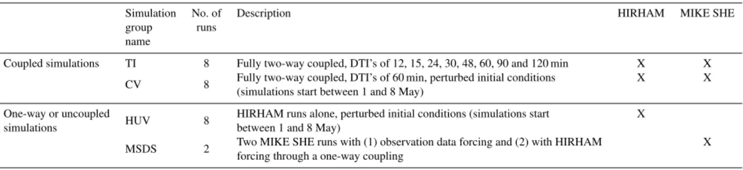
Table 1.Simulation outline showing simulation groups, number of runs in each group and short description of simulation group characteris-tics. The two latter columns show from which of the two model components the simulation output derives.
Simulation No. of Description HIRHAM MIKE SHE
group runs
name
Coupled simulations TI 8 Fully two-way coupled, DTI’s of 12, 15, 24, 30, 48, 60, 90 and 120 min X X CV 8 Fully two-way coupled, DTI’s of 60 min, perturbed initial conditions X X
(simulations start between 1 and 8 May) One-way or uncoupled
HUV 8 HIRHAM runs alone, perturbed initial conditions (simulations start X
simulations between 1 and 8 May)
MSDS 2 Two MIKE SHE runs with (1) observation data forcing and (2) with HIRHAM X forcing through a one-way coupling
2.6 Simulations
All model simulations were performed for the 1-year period from 1 May 2009 to 30 April 2010 with a spin-up period from the beginning of March to 30 April 2009. A total of 26 model runs were used; in the present study they are divided into four main categories (see also Table 1):
– Transfer interval (TI): eight two-way fully coupled sim-ulations were performed by varying the DTI, between the HIRHAM and MIKE SHE models, between 12 and 120 min. These DTI values were chosen to conform to time step restrictions imposed by MIKE SHE (given in fractions of an hour) to ensure accurate process mod-elling and to allow for executing model runs within the time slots allocated by the supercomputing facility at the Danish Meteorological Institute. The TI runs used 1 March 2009 as the starting day.
– HIRHAM uncoupled variability (HUV): eight HIRHAM uncoupled simulations were performed each starting 1 day apart from 1 to 8 March 2009.
– Coupled variability (CV): eight two-way fully coupled simulations using a 60 min DTI were performed using starting dates from 1 to 8 March 2009 as above.
– MIKE SHE data source (MSDS): to assess the influ-ence of data sources on MIKE SHE performance two MIKE SHE simulations were performed. (1) Uncoupled mode using observed values of PRECIP, RH,V,Rg,Ta
andPsand (2) one-way coupled mode using simulated
values as driving variables based on HIRHAM model simulations with 30 min DTI and without feedback to HIRHAM.
The eight uncoupled HIRHAM runs all show varying geo-graphical and temporal patterns of, in particular, precipita-tion. With these changes in precipitation, the water available for evapotranspiration and the energy balance is altered and, therefore, attention should be given to which simulations are compared. For all model runs, simulation output from
HIRHAM were assessed for the six climatic variables PRE-CIP, RH,V,Rg,TaandPs, since observations were available.
The same observational data were also used as input to MIKE SHE SWET for the uncoupled runs. Likewise, the output from the MIKE SHE simulations was assessed by compar-ing measurements of LE,HandGat the agricultural, forest and meadow sites (Fig. 1) as well as discharge measurements from three gauging stations.
Figure 2 outlines the data flow and simulation categories. As the Skjern catchment has an irregular shape, different de-grees of overlap are found between the HIRHAM grid cells and the hydrological catchment (Fig. 1). Analyses of PRE-CIP, RH,V,Rg,TaandPswere therefore performed for five
domains that reflect these different degrees of overlap: – Dom1: cells with 100 % overlap (nine cells);
– Dom2: Dom1+the cells with 50–100 % overlap (23 cells);
– Dom3: Dom2+the cells with 0–50 % overlap (30 cells);
– Dom4: Dom3+cells located immediately downstream of the catchment with regards to the dominant western wind direction (42 cells);
– Dom5: a cluster of cells east of the coupled catchment (four cells).
For HIRHAM output, the evaluation was performed on all five test domains by calculating a single root-mean-square er-ror (RMSE) value for each full model simulation. For MIKE SHE output, the RMSE was performed on the point data only. The RMSE was calculated on the basis of hourly values of RH,V,Rg,Ta,Ps, LE, H andGand daily values of
PRE-CIP andQagainst the corresponding observations for the six HIRHAM and four MIKE SHE variables:
RMSE=
v u u t
P
i,t
SIMi, t−OBSi,t2
n (1)
Figure 2.Flow chart of the data flow and analyses performed in the present study, and a legend of the variables mentioned in the study.
is the total number of data points. To assess the output vari-ability from each of the three simulation groups involving HIRHAM (TI, CV and HUV), simulation box plots with the 25th and 75th percentiles including whiskers for the most ex-treme data were created (Figs. 5 and 8).
Similarly, the mean absolute errors (MAE) were assessed to gain more information on the expected improvements for simulations with a more frequent DTI:
MAE=
P
i,t
|SIMi,t−OBSi,t|
n (2)
where the terms correspond to the RMSE calculations. The MAE calculations, for the TI simulations, were performed for each of the six HIRHAM variables over each of the five test domains and the four MIKE SHE variables at point scale. Linear trend lines, using least squares, were then fitted to the 12–120 min DTI MAE values for each of the test domains and point scale output and for each variable. The mean ab-solute and percentage change in MAE, based on the trend lines from the 120 min to the 12 min data points, were then calculated. Also, correlation coefficients on the basis of the trend lines were calculated to detect statistical significance at a 95 % two-tailed level.
The HUV and CV simulation groups apply the same changes in initial conditions by using different start dates to perturb these initial conditions but differ by having different land-surface schemes over the Skjern catchment. These sim-ulations were therefore used to test for statistical significance of the coupling. A simple two-samplet test was performed for each of the test domains and variables for the HUV and CV simulations to test the hypothesis of these simulation groups having unequal means.
3 Results
3.1 HIRHAM output
3.1.1 Data transfer interval (DTI)
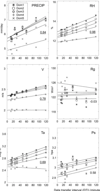
Of the six HIRHAM output variables, the four variables of PRECIP, RH,V andTashow a significant decrease in RMSE
with decreasing DTI in the fully two-way coupled mode sim-ulations, whereas Ps is less affected and Rg is unaffected
(Fig. 3). Based on the linear trend line averages between the domains, RMSE improvements of 1.1 mm day−1, 1.1 %,
0.2 m s−1 and 0.3◦C are seen for PRECIP, RH, V andT a,
Figure 3.HIRHAM output RMSE statistics for each of the test do-mains for the coupled TI simulations. Linear trend lines are shown with RMSE as a function of DTI as well as the average trend line correlation coefficients where the significant correlations on a two-sided 95 % confidence level are underlined.
of 0.3 mm day−1, 0.8 %,−0.1 m s−1and 0.2 corresponding
to a change from the 120 to the 12 min simulations of 7.2 % averaged for the four significant variables (Table 2). For the variables with statistically significant trends, PRECIP, RH,V andTa, there is a specific order in the resulting RMSE trend
line locations with the largest RMSE values for Dom1, Dom2 etc., decreasing down to Dom5.
The execution time for the coupled set-up, as a function of DTI, is shown in Fig. 4. Only a moderate increase in ex-ecution time is seen in the range of 60–120 min DTI values
Figure 4.Model execution time in hours of wall time as a func-tion of DTI. DTI steps of 6, 9, 12, 15, 24, 30, 48, 60, 90 (eight CV runs), and 120 min were used, whereas 6 and 9 min DTI values were extrapolated from unfinished runs. For comparison, the dashed line is the execution time for the uncoupled HIRHAM runs (HUV). Reprinted from Butts et al. (2014).
whereas a sharp increase is seen from DTI values of around 15–30 min.
3.1.2 HIRHAM model variability
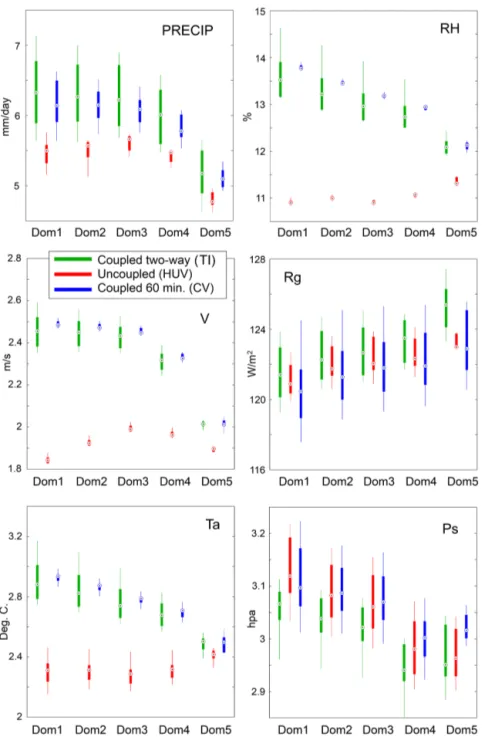
Figure 5 shows the output variability for each of the TI, CV and HUV group runs for each of the five test domains, Dom1–Dom5. For PRECIP, RH,V and to some extentTa, the
largest variability is seen for the two-way coupled runs (TI). The RH andV, using a 60 min DTI, for both the CV and HUV runs show almost negligible variability. For PRECIP, the CV variability is greater than for HUV whereas the oppo-site is the case forTawith a larger variability in the HUV
sim-ulations. For the variables, PRECIP, RH,V andTa, a general
decrease in RMSE is seen for the coupled TI and CV sim-ulations with increasing test domain number from Dom1 to Dom5. For the HUV simulations, this pattern is seen, to some extent, for PRECIP only. TheRgandPsvariables show
com-parable levels of variability between the TI, CV and HUV simulation groups. ForRg, the RMSE values increase with
test domain number, whereas the opposite is the case forPs.
When comparing the influence of variability with the influ-ence of DTI it is seen that the range in RMSE values from the perturbation induced HUV variability corresponds to 47 % of the RMSE improvement for the TI simulations when going from 120 to 12 min (based on the linear trend lines). The cor-responding number when comparing TI with CV is 46 %.
Two-samplet tests confirmed the hypotheses that the re-sults from the HUV and CV simulations belong to two sep-arate populations for the variables PRECIP, RH,V andTa
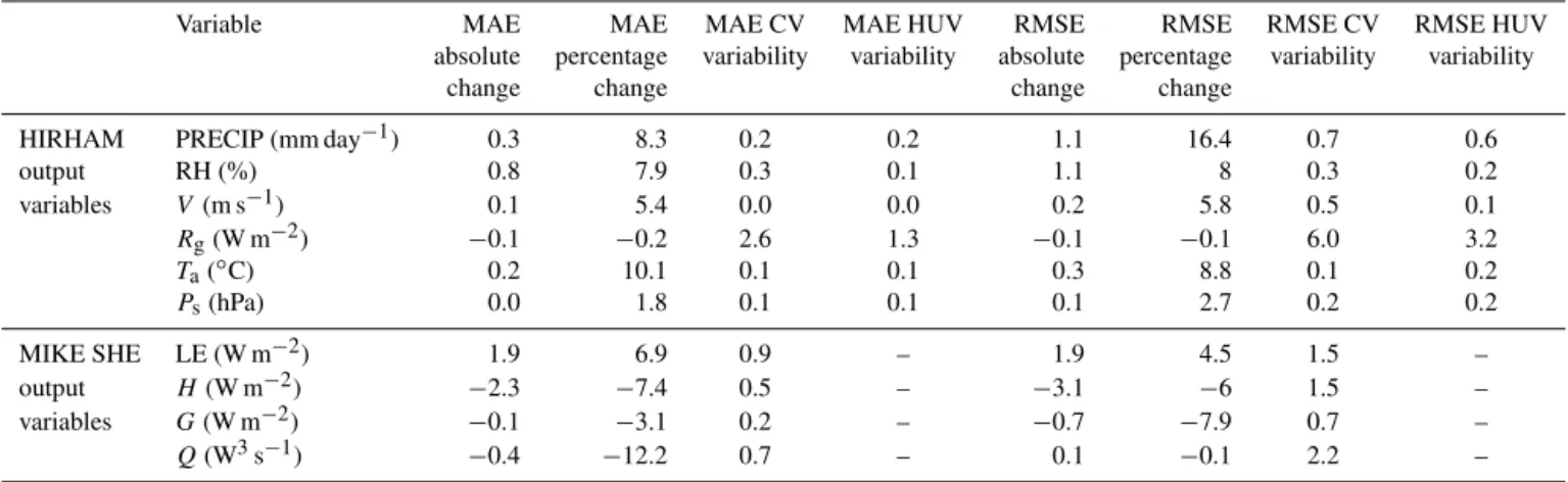
Table 2.Absolute and percentage change in MAE and RMSE between the largest (120 min) and smallest (12 min) DTI based on the average value of the linear trend lines of either the five test domains (HIRHAM output) or the measurement sites (MIKE SHE output). Also shown is the absolute variability from the CV and HUV runs defined as the minimum value subtracted from the maximum for the 60 min DTI averaged between test domains (HIRHAM output) or measurement sites (MIKE SHE output) for each tested variable.
Variable MAE MAE MAE CV MAE HUV RMSE RMSE RMSE CV RMSE HUV absolute percentage variability variability absolute percentage variability variability
change change change change
HIRHAM PRECIP (mm day−1) 0.3 8.3 0.2 0.2 1.1 16.4 0.7 0.6
output RH (%) 0.8 7.9 0.3 0.1 1.1 8 0.3 0.2
variables V(m s−1) 0.1 5.4 0.0 0.0 0.2 5.8 0.5 0.1
Rg(W m−2) −0.1 −0.2 2.6 1.3 −0.1 −0.1 6.0 3.2
Ta(◦C) 0.2 10.1 0.1 0.1 0.3 8.8 0.1 0.2
Ps(hPa) 0.0 1.8 0.1 0.1 0.1 2.7 0.2 0.2
MIKE SHE LE (W m−2) 1.9 6.9 0.9 – 1.9 4.5 1.5 – output H(W m−2) −2.3 −7.4 0.5 – −3.1 −6 1.5 – variables G(W m−2) −0.1 −3.1 0.2 – −0.7 −7.9 0.7 – Q(W3s−1) −0.4 −12.2 0.7 – 0.1 −0.1 2.2 –
Figure 6 shows the simulated PRECIP for each run of the TI, HUV and CV simulation groups and for each test do-main. PRECIP is seen to decrease with increasing domain number for all three simulation groups, as well as for obser-vations. This decrease is strongest for the two-way coupled TI and CV simulation groups, which also show the high-est PRECIP levels compared to the uncoupled HUV simu-lations. Compared to the observed PRECIP mean over the five test domains of 892 mm over the simulation period, both the TI and CV simulations consistently overestimate PRE-CIP with accumulated values of 1004 and 1027 mm, respec-tively. In contrast, the HUV underestimates the PRECIP for this period, with an accumulated value of 868 mm. Despite generally overestimating the rainfall, the coupled TI runs, with high frequency DTIs and a high degree of coupling (Dom1–Dom3), show better estimates of accumulated rain-fall compared to uncoupled run (CV). With regard to timing, there is a tendency for the main part of the TI simulation variability to arise from events in the fall months of 2009, whereas most of the HUV and CV variability occurs in early 2010 events.
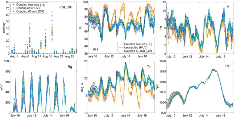
In addition to comparing simulation statistics and precipi-tation accumulation plots, the HIRHAM output variables for all 24 TI, HUV and CV simulations are plotted in Fig. 7. This figure shows hourly values for the period 10–17 July 2009, with the exception of precipitation data which are given as daily values for all of August 2009. The 1-week period was chosen to reflect high dynamics in the peak summer period, whereas the 1-month period of august showed more itation compared to July. A large spread is seen for precip-itation amounts on individual days that appears to increase with the mean intensity, most pronounced on 10 and 20 Au-gust. Reasonable agreement is seen between these simula-tions in terms of capturing the dry days. For the remaining five variables, RH,Ta,Psand especiallyV andRg, the period
with low pressure and precipitation, 10–12 July, exhibits a fair amount of spread between the individual simulations, whereas the remaining period, 13–17 July, shows a higher de-gree of consistency within each simulation group (TI, HUV and CV) especially in terms of dynamics. For the PRECIP, RH,V andTavariables the coupled simulations groups of TI
and CV clearly deviate from the HUV simulations in terms of the timing, dynamics and absolute levels. Of these, the most noticeable difference is the daytime RH and night-time Ta, which are notably higher and lower, respectively, for the
HUV simulations.
3.2 MIKE SHE output
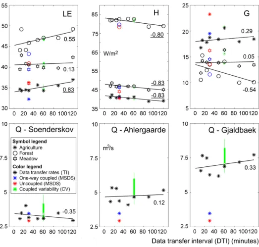
As for the HIRHAM simulations, the MIKE SHE RMSE re-sults are plotted as a function of DTI (Fig. 8). LE shows a general improvement in RMSE with a higher frequency of exchange (smaller DTI), which is strongest for the agricul-ture and forest sites. Correlation coefficients between RMSE and DTI of 0.83, 0.55 and 0.13 are found for the agriculture, forest and meadow sites respectively. Conversely,H shows general decreases in RMSE with increased DTI and with cor-relation coefficients of−0.80 to−0.83. The changes in LE andH thereby represent opposing signals which could be expected, to some degree, from the conservation of the en-ergy balance. No clear trend between DTI and RMSE results is seen for bothGandQand the corresponding correlation coefficients are generally low.
For LE, an absolute improvement of 1.9 W m−2 in both
Figure 5.RMSE variability for the TI, HUV and CV simulations for each of the five test domains. The dots represent the median value, the box plots represent the 25–75th percentiles and the whiskers represent the entire data range.
MIKE SHE RMSE total output span of 1.5, 1.5, 0.7 W m−2
and 2.2 m3s−1for LE,H,GandQas an average of the three surfaces and the three discharge stations (Fig. 8). By compar-ison, the TI simulations induce a spread in the corresponding results, not based on the trend lines as in Table 2, of 3.7, 3.8, 4.5 W m−2and 1.3 m3s−1, respectively.
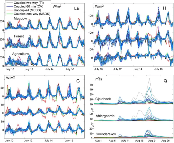
The variations in the MIKE SHE output for four vari-ables LE,H,GandQ, for the CV and TI model runs, are shown in Fig. 9. There is also no distinct pattern distinguish-ing the TI and CV simulation group results. The simulations
Figure 6.Precipitation sum curve for the evaluation period 1 May 2009 to 30 April 2010 for the five test domains and the TI, HUV and CV simulations as well as the observations. Also given are the simulated mean values, the span in the period sum for each plot group (minimum value subtracted from maximum value) and the observed mean values.
observation data, especially for night-time LE and G, than the TI and CV runs. It should be pointed out that for this anal-ysis (Fig. 9), although results are extracted from three single MIKE SHE cells (for meadow, forest and agriculture), the forcing data are based on either 11 km resolution HIRHAM data input (TI and CV) or 10 km observation gridded data (station interpolated – MSDS), which can be expected to smooth out local features.
4 Discussion
The motivation for performing this coupling study is to in-clude the land-surface–atmosphere interactions between the RCM and the hydrological model. Our hypothesis is that the RCM will benefit from the more detailed representation of the surface and subsurface processes provided by the ded-icated hydrological model as compared to the much sim-pler land-surface schemes that climate models usually rely on. Similarly, we expect that the hydrological model would
benefit from the better representation of the horizontal re-distribution processes in the atmosphere offered by dynamic coupling with the climate model.
4.1 Performance of coupled versus uncoupled model It is not surprising that the performance of the coupled model simulations (TI and CV), when compared to hourly values of RH, V and Ta and daily PRECIP, is generally poorer
Figure 7.The six HIRHAM output variables assessed in the present study in the 10–17 July period (precipitation is 1–31 August to match the period in Fig. 9 with a higher dynamic in discharge) for all 24 TI, HUV and CV runs and for Dom1 (nine cell mean). The legend colouring reflects the overall simulation group (TI, HUV or CV) whereas each simulation is in the colour shade as in Fig. 6.
land-surface scheme in HIRHAM is replaced by MIKE SHE SWET over the Skjern catchment. Calibration or parameter tuning of complex models comprising several processes of-ten introduces compensational errors (i.e. providing the right answer for the wrong reason) in the different model compo-nents in order to ensure the model fits observational data as well as possible (Graham and Jacob, 2000). When the exist-ing land-surface scheme in HIRHAM is replaced by MIKE SHE SWET, it will inevitably provide different results likely to be poorer in terms of a hindcast assessment. We should, however, highlight that the coupled system shows benefits over the uncoupled when assessing longer-term periods such as cumulative precipitation where high frequency DTI’s pro-duce better results (Fig. 6). Also, greater accuracy in the rep-resentation of soil moisture and water available for evapo-transpiration, in the coupled system, could explain these find-ings. In terms of future climate projections, which are typ-ically in the range of 10–30-year integrations, this is very promising and suggests there could be potential added value in using the coupled model system. Similar results, where the added complexity when joining two existing model systems does not lead to obvious direct improvements in simulations, has also been seen in studies of coupling ocean models and atmosphere models (Covey et al., 2004).
From a different perspective the fact that the hourly to daily coupled model performance in many respects is poorer, when replacing the existing land-surface scheme with a more elaborate and well-calibrated one (MIKE SHE SWET),
suggests that some of the HIRHAM components could be improved. So far very few attempts have been made in for-malized calibration of RCMs, and we are not aware of any study that aims at calibrating coupled hydrology-RCM mod-els. While there is a very interesting perspective here in a formal calibration of HIRHAM, such as presented by Bell-prat et al. (2012), and in learning from the coupled model to improve the HIRHAM parameterizations, this is outside the scope of the current study.
To some degree the atmospheric variables are likely to be affected by the discontinuity in model physics between HIRHAM uncoupled cells and MIKE SHE coupled cells for the present version of the modelling set-up. With the current experimental set-up it was, however, not possible to distinguish between this effect and the change in land-surface signal from MIKE SHE as opposed to the inherent HIRHAM land-surface scheme signal. Large differences in surface fluxes between neighbouring grid cells both inside and outside the coupled area are nonetheless seen, as induced by differences in vegetation, soil, topography etc., and dis-continuities at the uncoupled–coupled interface are therefore not considered important.
4.2 DTI
Figure 8.MIKE SHE output RMSE statistics for each of the three flux tower measurement sites and the three discharge stations for the TI, MSDS and CV simulations. For the TI simulations linear trend lines are shown with RMSE as a function of DTI as well as the average trend line correlation coefficients where significant correlations on a two-sided 95 % confidence level are underlined. Also, the variability of the perturbed CV simulations is shown.
is highly relevant for studies over longer periods. This improved performance of the coupled set-up is constrained, however, by a corresponding increase in computation time. The general decrease in RMSE levels with lower DTI is not surprising as a more frequent update of the surface forc-ing from MIKE SHE will include more dynamic features in the land-surface exchange and better align with variations in the surface energy balance affecting the land–atmosphere interaction. To fully capture the higher degree of dynamics in the land-surface–atmosphere interaction and dependence during unstable atmospheric conditions, a high frequency DTI closer to the RCM time step is likely to be important. One might suspect the effect of DTI to level off when ap-proaching the internal HIRHAM model time step of 120 s and to obtain results affected by coupling features alone. Along these lines, a more dynamic pattern is seen for most variables for days with a higher degree of cloud cover and lowerRglevels (10 and 17 July; Fig. 7).
Similar to this study Maxwell et al. (2011) have tested the timing of data transfer between the ParFlow hydrological model and the WRF atmospheric model in a 48 h idealized
constructed set-up. The simulations were performed by us-ing four transfer intervals of 5, 10, 60 and 360 s, where WRF used a constant time step of 5 s (non-hydrostatic model) and the time step in ParFlow varied with the TI. Good water bal-ance results were obtained for transfer rates up to 12 times that of WRF (60 s), whereas the results for TI of 360 s de-teriorated. Even though a smaller time step was used in WRF than in HIRHAM in the present study (5 s compared to 120 s), the results of Maxwell et al. (2011) correspond rea-sonably well to our results, where a transfer rate of 12 times that of HIRHAM would correspond to a 24 min DTI.
4.3 Impact of coupling evaluated against climate model variability
Figure 9.Four MIKE SHE output variables for the period 10–17 July (discharge is 1–31 August) for the TI, CV and MSDS runs and for Dom1 (nine cell mean). The legend colouring reflects the overall simulation group (TI, CV and MSDS) and each simulation has the same colour shade as in Fig. 6. The individual flux sites are shown for LE only. Notice theyaxis shifts to accommodate more sites.
critically recommendable to explore variations caused by the physical changes (i.e. the coupling) as opposed to the in-ternal climate model variation when developing coupled cli-mate–hydrology modelling systems.
In our study, the precipitation amounts spanning 75–99 and 52–134 mm for the HUV and CV simulations re-spectively, exhibit a significant variability in simulated PRE-CIP simply as a result of changes in the initial conditions. This has also been shown in several other studies (Casati et al., 2004; van de Beek et al., 2011; Larsen et al., 2013), which have highlighted the importance of considering cli-mate model variability when assessing model performance. In the present case the coupling is seen to inflate the vari-ability of local precipitation as compared to the uncoupled climate model simulations even considering internal climate model variability. Since many climate models generally tend to underestimate the variability of local precipitation, thus providing unrealistic projections of events, such as extreme precipitation, this is again a potentially promising feature of a coupled model system, e.g. with respect to the represen-tation of long-term trends in precipirepresen-tation for longer periods
(multiple years) and in future climate projections, and will be investigated in future studies.
4.4 Test domains
There is a clear tendency for increased RMSE levels from the TI simulations with a higher degree of coupling from Dom1 to Dom5 with the exception ofRgresults (Fig. 3). An
coastline has also been shown to affect precipitation results from HIRHAM (Larsen et al., 2013) and thereby the avail-able water affecting the energy balance budget. In this regard, the test domains Dom2 and specifically Dom3–Dom4 are lo-cated close to Ringkøbing Fjord, which might contribute to the higher RMSE levels of these compared to Dom5.
4.5 Scale of variables
An essential consideration is to assess at which spatial scale the atmospheric variables are affected by the land-surface model. The Skjern River catchment covers an area of approx-imately 70 km×50 km, and our hypothesis is that areas in the proximity of the catchment and up to 25 km downstream of the catchment (in relation to the dominant wind direction) may be affected by the model coupling. This corresponds to atmospheric scales from smaller mesoscale to microscale. It could be argued, however, that the effect of the coupling, al-though tested on regional scales below 100 km, could likely be imposed regionally on top of larger scale atmospheric phe-nomena such as larger mesoscale and synoptic scale features. In this regard it should be noted that global incoming solar ra-diation (Rg) which is, by and large, affected by cloud cover
and therefore by upstream larger meso- and synoptic scale conditions, shows no effect of the coupling scenario, as the RMSE pattern resembles a somewhat random pattern as a function of DTI, test domain and model variability (Fig. 3). Similarly, Ps would be connected with larger scale weather
systems and sea surface temperatures (Køltzow et al., 2011) and is seen to be constrained, to some degree, by lateral boundary conditions (Seth and Georgi, 1998; Diaconescu et al., 2007; Leduc and Laprise, 2009) but is highly influenced by domain characteristics (Larsen et al., 2013). The variables RH, V andTa all vary on spatial scales far below the
reso-lution of HIRHAM and even MIKE SHE and the improved results with a more frequent DTI could therefore be antici-pated to some extent. Also PRECIP, in particular convective rainfall, can be seen at grid scales below the HIRHAM reso-lution (Casati et al., 2004).
Another potential contribution to the coupled model per-formance comes from the fact that HIRHAM is a hydro-static RCM with a convective scheme close to, or at, the threshold of its minimum resolution as also suggested in Larsen et al. (2013). Although, HIRHAM has been tested at similar spatial scales previously and was found to provide reasonable results, at very fine temporal scales the hydro-static nature of HIRHAM could arguably contribute to the degree of variability seen for precipitation, and the 11 km resolution naturally has its limits compared to newer stud-ies utilizing atmospheric model resolutions of a few kilome-tres, such as Kendon et al. (2014). For hydrological stud-ies forcing data having finer resolutions are highly benefi-cial (Xue et al., 2014) and must be expected even more im-portant for regions with a complex topography and a high degree of convective precipitation. One approach to reach
fine resolutions appropriate for hydrological studies is seen in Berg et al. (2012) using a range of downscaling meth-ods to achieve a resolution of 1 km over a northern Euro-pean region thereby demonstrating significant improvements for both temperature and precipitation. Conversely, the un-certainty related to events such as the location and timing of precipitation, are in general much larger than the model res-olution even for very high resres-olution non-hydrostatic mod-els, particularly at the time scales of climate projections (Rasmussen et al., 2012). Hence, in practical terms, the HIRHAM-MIKE SHE set-up explored in this paper repre-sents a reasonable compromise in terms of delivering results of sufficient spatial representation for a number of problems in climate projection studies.
4.6 Perspectives for further use
Computationally, we show that it is feasible to run simula-tions using coupled models dedicated to different types of computing systems, in this case a high performance com-puter and a personal comcom-puter. Moreover, we have demon-strated that transient coupled climate–hydrology simulations at the decadal scale or longer is well within reach. The present prototype implements a number of technical deci-sions inherent to the computing environment available for this study and more work is needed in order to reduce computation times, e.g. implementation of a more efficient memory-based data transmission scheme as prescribed in the OpenMI standard. In its current form, the coupling approach, however, may easily be generalized to other computing envi-ronments. In terms of further model development this work suggests that several steps may be undertaken to improve the coupled model performance. While we directly link model variables in the present study using an OpenMI interface, the present framework could easily be extended by imposing em-pirical downscaling and bias correction methods to further improve model compatibility across time and spatial scales.
5 Conclusions
This study presents the performance of the fully two-way coupled set-up between the HIRHAM RCM and the combined MIKE SHE/SWET hydrological and land-surface models. In particular, the influence of the DTI between the models, the domain of coupling influence and the HIRHAM model variability, was assessed.
Of the six HIRHAM output climate variables PRECIP, RH,V andTashowed significant differences between
difficult variables to simulate. TheRgandPsvariables were
shown to have little to no impact from the coupling. Little to no improvement in the MIKE SHE output variables is seen for decreased DTI values as the improvement in LE is in the same range as theHdecline.
The uncoupled and coupled HIRHAM model variability, induced by perturbing the HIRHAM runs with varying start-ing dates, was shown to correspond to 47 and 46 %, respec-tively, of the average improvements in RMSE and MAE for the four significant variables when going from a 120 min to a 12 min DTI. Similarly significant variations were seen in the simulated precipitation where the eight two-way fully coupled simulations with 12 to 120 min DTI values (TI) produced spans in precipitation during the 1 year period of 108–170 mm for the five test domains. Similarly, the uncou-pled (HUV) and couuncou-pled (CV) simulations where model vari-ability was induced by changing initial conditions showed precipitation spans of 75–99 and 52–134 mm, respectively. For all of these, the resulting span increased with a higher degree of coupling. Part of this pattern may be attributed to well-known geographical HIRHAM bias over the central Jut-land ridge. The HIRHAM model variability as transferred to the MIKE SHE model in the 60 min DTI CV simulations were substantially higher for discharge than for the LE,Hor Gheat fluxes.
In general, the coupled modelling results (TI and CV) are poorer than the uncoupled results (HUV) when assessed on a sub-daily to daily basis, whereas longer-term precipitation is better reproduced by more frequent DTI coupled simula-tions. The poorer short-term coupled performance is not sur-prising as each of the models over the years, also prior to this study, have been separately refined (convective scheme and land-surface energy balance) or calibrated to accurately reproduce observations. These calibrations are likely to have compensated for errors in the separate and complex model components to ensure a proper data fit. We suggest that the replacement of the land-surface scheme in HIRHAM, as in-troduced by MIKE SHE, and the change in data input in MIKE SHE, as introduced by HIRHAM, causes this deterio-ration. A potential calibration of the coupled set-up is outside the time frame and scope of the present paper, however we see a great potential for further improvements.
Acknowledgements. The present study was funded by grants from the Danish Strategic Research Council for the project Hydrological Modelling for Assessing Climate Change Impacts at Different Scales (HYACINTS – www.hyacints.dk) under contract no. DSF-EnMi 2104-07-0008 and the project Centre for Regional Change in the Earth system (CRES – www.cres-centre.dk) under contract no. DSF-EnMi 09-066868. The present study is made possible through a collaboration with the HOBE project (www.hobecenter.dk) funded by the Villum Kann Rasmussen Foundation.
Edited by: E. Zehe
References
Alexandru, A., Elia, R. D., and Laprisé, R.: Internal Variability in Regional Climate Downscaling at the Seasonal Scale, Mon. Weather Rev., 135, 3221–3238, doi:10.1175/MWR3456.1, 2007. Allerup, P., Madsen, H., and Vejen, F.: Standardværdier (1961–90) af Nedbørkorrektioner, Danish Meteorological Institute Techni-cal Report 98-10, Danish MeteorologiTechni-cal Institute, Copenhagen, 1998.
Anyah, R. O., Weaver, C. P., Miguez Macho, G., Fan, Y., and Robock, A.: Incorporating water table dynamics in cli-mate modeling: 3. Simulated groundwater influence on coupled land-atmosphere Variability, J. Geophys. Res., 113, DO7103, doi:10.1029/2007JD009087, 2008.
Bellprat, O., Kotlarski, S., Lüthi, D., and Schär, C.: Objective calibration of regional climate models, J. Geophys. Res., 117, D23115, doi:10.1029/2012JD018262, 2012.
Berg, P., Feldmann, H., and Panitz, H.-J.: Bias correction of high resolution regional climate model data, J. Hydrol., 448–449, 80–92, doi:10.1016/j.jhydrol.2012.04.026, 2012.
Butts, M., Drews, M., Larsen, M. A. D., Lerer, S., Rasmussen, S. H., Gross, J., Overgaard, J., Refsgaard, J. C., Christensen, O. B., and Christensen, J. H.: Embedding complex hydrology in the regional climate system – dynamic coupling across dif-ferent modelling domains, Adv. Water Resour., 74, 166–184, doi:10.1016/j.advwatres.2014.09.004, 2014.
Casati, B., Ross, G., and Stephenson, D. B.: A new intensity-scale approach for the verification of spatial precipitation forecasts, Meteorol. Appl., 11, 141–154, doi:10.1017/S1350482704001239, 2004.
Caya, D. and Laprise, R.: A semi-implicit semi-Lagrangian regional climate model: The Canadian RCM, Mon. Weather Rev., 127, 341–362, 1999.
Christensen, J. H., Christensen, O. B., Lopez, P., van Meijgaard, E., and Botzet, M.: The HIRHAM4 Regional Atmospheric Climate Model, Danish Meteorological Institute Technical Report 96-4, Danish Meteorological Institute, Copenhagen, 1996.
Christensen, O. B., Drews, M., Christensen, J. H., Dethloff, K., Ke-telsen, K., Hebestadt, I., and Rinke, A.: The HIRHAM regional climate model version 5, Danish Meteorological Institute Techni-cal Report 06-17, Danish MeteorologiTechni-cal Institute, Copenhagen, 2006.
Covey, C., Achutarao, K. M., Gleckler, P. J., Phillips, T. J., Taylor, K. E., and Wehner, M. F.: Coupled ocean-atmosphere climate simulations compared with simulations using prescribed sea sur-face temperature: effect of a “perfect ocean”, Global Planet. Change, 41, 1–14, doi:10.1016/j.gloplacha.2003.09.003, 2004. Cui, X., Graf, H.-F., Langmann, B., Chen, W., and Huang,
R.: Climate impacts of anthropogenic land use changes on the Tibetan Plateau, Global Planet. Change, 54, 33–56, doi:10.1016/j.gloplacha.2005.07.006, 2006.
Diaconescu, E. P., Laprise, R., and Sushama, L.: The impact of lateral boundary data errors on the simulated climate of a nested regional climate model, Clim. Dynam., 28, 333–350, doi:10.1007/s00382-006-0189-6, 2007.
Gerten, D., Schaphoff, S., Haberlandt, U., Lucht, W., and Sitch, S.: Terrestrial vegetation and water balance – hydrological eval-uation of a dynamic global vegetation model, J. Hydrol., 286, 249–270, doi:10.1016/j.jhydrol.2003.09.029, 2004.
Giorgi, F. and Bi, X.: A study of internal variability of a regional climate model, J. Geophys. Res., 105, 29503–29521, 2000. Goodall, J. L., Saint, K. D., Ercan, M. B., Briley, L. J.,
Murphy, S., You, H., DeLuca, C., and Rood, R. B.: Coupling climate and hydrological models: Interoperability through Web Services. Environ. Modell. Softw., 46, 250–259, doi:10.1016/j.envsoft.2013.03.019, 2013.
Graham, D. N. and Butts, M. B.: Flexible, integrated watershed modelling with MIKE SHE, in: Watershed Models, edited by: Singh, V. P. and Frevert, D. K., CRC Press, Boca Raton, Florida, USA, 245–272, 2005.
Graham, L. P. and Jacob, D.: Using large-scale hydrologic modeling to review runoff generation processes in GCM climate models, Meteorol. Z., 9, 49–57, 2000.
Gregersen, J. B., Gijsbers, P. J. A., Westen, S. J. P., and Blind, M.: OpenMI: the essential concepts and their implications for legacy software, Adv. Geosci., 4, 37–44, doi:10.5194/adgeo-4-37-2005, 2005.
Gregersen, J. B., Gijsbers, P. J. A., and Westen, S. J. P.: Open modelling interface, J. Hydroinform., 9, 175–191, doi:10.2166/hydro.2007.023, 2007.
Højberg, A. L., Troldborg, L., Stisen, S., Christensen, B. S. B., and Henriksen, H. J.: Stakeholder driven update and improvement of a national water resources model. Environ. Modell. Softw., 40, 202-213, doi:10.1016/j.envsoft.2012.09.010, 2013.
Jacob, D., Bärring, L., Christensen, O. B., Christensen, J. H., De Castro, M., Déqué, M., Giorgi, F., Hagemann, S., Hirschi, M., Jones, R., Kjellström, E., Lenderink, G., Rockel, B., Sánchez, E., Schär, C., Seneviratne, S. L., Somot, S., Van Ulden, A. P., and Van Den Hurk, B. J. J. M.: An inter-comparison of regional climate models for Europe: model performance in present-day climate, Climatic Change, 81, 31–52, doi:10.1007/s10584-006-9213-4, 2007.
Jiang, X., Niu, G.-Y., and Yang, Z.-L.: Impacts of vegetation and groundwater dynamics on warm season precipitation over the Central United States, J. Geophys. Res., 114, DO6109, doi:10.1029/2008JD010756, 2009.
Kendon, E. J., Roberts, N. M., Fowler, H. J., Roberts, M. J., Chan, S. C., and Senior, C. A.: Heavier summer downpours with climate change revealed by weather forecast resolution model, Nat. Clim. Change, 4, 570–576, doi:10.1038/NCLIMATE2258, 2014. Kjellström, E., Bärring, L., Jacob, D., Jones, R., Lenderink, G., and
Schär, C.: Modelling daily temperature extremes: recent climate and future changes over Europe, Climatic Change, 81, 249–265, doi:10.1007/s10584-006-9220-5, 2007.
Klüpfel, V. Kalthoff, N., Gantner, L., and Kottmeier, C.: Eval-uation of soil moisture ensemble runs to estimate pre-cipitation variability in convection-permitting model sim-ulations for West Africa, Atmos. Res., 101, 178–193, doi:10.1016/j.atmosres.2011.02.008, 2011.
Kollet, S. J. and Maxwell, R. M.: Capturing the influence of ground-water dynamics on land surface processes using an integrated, distributed watershed model, Water Resour. Res., 44, W02402, doi:10.1029/2007WR006004, 2008.
Køltzow, M. A. Ø., Iversen, T., and Haugen, J. E.: The Importance of Lateral Boundaries, Surface Forcing and Choice of Domain Size On the role of domain size and resolution in the simulations for Dynamical Downscaling of Global Climate Simulations, At-mosphere, 2, 67–95, doi:10.3390/atmos2020067, 2011. Kunstmann, H. and Stadler, C.: High resolution distributed
atmospheric-hydrological modelling for Alpine catchments, J. Hydrol., 314, 105–124, doi:10.1016/j.jhydrol.2005.03.033, 2005.
Larsen, M. A. D., Thejll, P., Christensen, J. H., Refsgaard, J. C., and Jensen, K. H.: On the role of domain size and resolution in the simulations with the HIRHAM region climate model, Clim. Dynam., 40, 2903–2918, doi:10.1007/s00382-012-1513-y, 2013. Larsen, M. A. D.: Integrated Climate And Hydrology Modelling – Coupling of the HIRHAM Regional Climate Model and the MIKE SHE Hydrological Model, PhD Thesis, The Faculty of Science, University of Copenhagen, Copenhagen, 2013. Leduc, M. and Laprise, R.: Regional climate model sensitivity to
domain size, Clim. Dynam., 32, 833–854, doi:10.1007/s00382-008-0400-z, 2009.
Maxwell, R. M., Chow, F. K., and Kollet, S. J.: The groundwater–land-surface–atmosphere connection: Soil mois-ture effects on the atmospheric boundary layer in fully-coupled simulations, Adv. Water Resour., 30, 2447–2466, doi:10.1016/j.advwatres.2007.05.018, 2007.
Maxwell, R. M., Lundquist, J. K., Mirocha, J. D., Smith, S. G., Wo-ordward, C. S., and Tompson, A. F. B.: Development of a Cou-pled Groundwater–Atmosphere Model, Mon. Weather Rev., 39, 96–116, doi:10.1175/2010MWR3392.1, 2011.
Overgaard, J.: Energy-based land-surface modelling: new opportu-nities in integrated hydrological modeling, Ph.D. Thesis, Insti-tute of Environment and Resources, DTU, Technical University of Denmark, Lyngby, 2005.
Plavcová, E. and Kyselý, J.: Evaluation of daily temperatures in Central Europe and their links to large-scale circulation in an ensemble of regional climate models, Tellus A, 63, 763–781, doi:10.1111/j.1600-0870.2011.00514.x, 2011.
Polanski, S., Rinke, A., and Dethloff, K.: Validation of the HIRHAM-Simulated Indian Summer Monsoon Circulation, Adv. Meteorol., 2010, 415632, doi:10.1155/2010/415632, 2010. Rasmussen, S. H.: Modelling land surface–atmosphere interactions, Ph.D. Thesis, University of Copenhagen, Department Of Geog-raphy and Geology, Copenhagen, 2012.
Rasmussen, S. H., Christensen, J. H., Drews, M., Gochis, D., and Refsgaard, J. C.: Spatial-Scale Characteristics of Precipitation Simulated by Regional Climate Models and the Implications for Hydrological Modeling, J. Hydrometeorol., 13, 1817–1835, doi:10.1175/JHM-D-12-07.1, 2012.
Ringgaard, R.: On variability of evapotranspiration – The role of surface type and vegetation, Ph.D. Thesis, University of Copen-hagen, Department Of Geography and Geology, CopenCopen-hagen, 2012.
Ringgaard, R., Herbst, M., Friborg, T., and Soegaard, H.: En-ergy Fluxes above Three Disparate Surfaces in a Temperate Mesoscale Coastal Catchment, Vadose Zone J., 10, 54–66, doi:10.2136/vzj2009.0181, 2011.
Tompkins, A.: Part 1. Model description. The atmospheric gen-eral circulation model ECHAM5, Report no. 349, Max-Planck-Institut für Meteorologie – MPI-M, Hamburg, 2003.
Seneviratne, S. I., Lüthi, D., Litschi, M., and Schär, C.: Land–atmosphere coupling and climate change in Europe, Na-ture, 443, 205–209, doi:10.1038/nature05095, 2006.
Seth, A. and Giorgi, F.: The effect of domain choice on summer pre-cipitation simulation and sensitivity in a regional climate model, J. Climate, 11, 2698–2712, 1998.
Shrestha, P., Sulis, M., Masbou, M., Kollet, S., and Simmer, C.: A Scale-Consistent Terrestrial Systems Modeling Platform Based on COSMO, CLM, and ParFlow, Mon. Weather Rev., 142, 3466–3483, doi:10.1175/MWR-D-14-00029.1, 2014.
Shuttleworth, W. J. and Wallace, J. S.: Evaporation from sparse crops – an energy combination theory, Q. J. Roy. Meteorol. Soc., 111, 839–855, 1985.
Skamarock, W. C., Klemp, J. B., Dudhia, J., Gill, O. D., Barker, D. M., Duda, M. G., Huang, X., Wang, W., and Powers, J. G.: A description of the Advanced Research WRF version 3, NCAR Techical Note NCAR/TN-4751STR, NCAR, Boulder, Colorado, USA, 2008.
Smiatek, G., Kunstmann, H., and Werhahn, J. Implementation and performance analysis of a high resolution coupled nu-merical weather and river runoff prediction model system for an Alpine catchment, Environ. Modell. Softw., 38, 231–243, doi:10.1016/j.envsoft.2012.06.001, 2012.
Stisen, S., McCabe, M. F., Refsgaard, J. C., Lerer, S., and Butts, M. B.: Model parameter analysis using remotely sensed pattern information in a multi-constraint framework, J. Hydrol., 409, 337–349, doi:10.1016/j.jhydrol.2011.08.030, 2011a.
Stisen, S., Sonnenborg, T., Højberg, A. L., Troldborg, L., and Ref-sgaard, J. C.: Evaluation of Climate Input Biases and Water Bal-ance Issues Using a Coupled Surface–Subsurface Model, Vadose Zone J., 10, 37–53, doi:10.2136/vzj2010.0001, 2011b.
Stisen, S., Højberg, A. L., Troldborg, L., Refsgaard, J. C., Chris-tensen, B. S. B., Olsen, M., and Henriksen, H. J.: On the impor-tance of appropriate precipitation gauge catch correction for hy-drological modelling at mid to high latitudes, Hydrol. Earth Syst. Sci., 16, 4157–4176, doi:10.5194/hess-16-4157-2012, 2012. Unden, P., Rontu, L., Järvinen, H., Lynch, P., Calvo, J., Cats, G.,
Cuxart, J., Eerola, K., Fortelius, C., Garcia-Moya, J. A., Jones, C., Lenderlink, G., Mcdonald, A., Mcgrath, R., Navascues, B., Nielsen, N. W., Degaard, V., Rodriguez, E., Rummukainen, M., Sattler, K., Sass, B. H., Savijarvi, H., Schreur, B. W., Sigg, R., and The, H.: HIRLAM-5 scientific documentation, HIRLAM Report, SMHI, Norrköping, Sweden, p. 144, 2002.
Uppala, S., Dee, S., Kobayashi, S., Berrisford, P., and Simmons, A.: Towards a climate data assimilation system: status update of ERA-Interim, ECMWF Newsletter No. 115, ECMWF, Reading, UK, 12–18, 2008.
van de Beek, C. Z., Leijnse, H., Torfs, P. J. J. F., and Uijlenhoet, R.: Climatology of daily rainfall semi-variance in The Netherlands, Hydrol. Earth Syst. Sci., 15, 171–183, doi:10.5194/hess-15-171-2011, 2011.
Xue, M., Droegemeier, K. K., and Wong, V.: The advanced regional prediction system (ARPS), A multi-scale non-hydrostatic atmo-spheric simulation and prediction model, Part I: model dynamics and verification, Meteorol. Atmos. Phys., 75, 161–193, 2000. Xue, M., Droegemeier, K. K., Wong, V., Shapiro, A., Brewster, A.,
Carr, F., Weber, D., Liu, Y., and Wang, D.: The advanced regional prediction system (ARPS), a multi-scale non-hydrostatic atmo-spheric simulation and prediction tool, Part II: model physics and applications, Meteorol. Atmos. Phys., 76, 143–165, 2001. Xue, Y., Janjic, Z., Dudhia, J., Vasic, R., and De Sales, F.:
A review on regional dynamical downscaling in intrasea-sonal to seaintrasea-sonal simulation/prediction and major factors that affect downscaling ability, Atmos. Res., 147–148, 68–85, doi:10.1016/j.atmosres.2014.05.0012014, 2014.
Yan, H., Wang, S. Q., Billesbach, D., Oechel, W., Zhang, J. H., Meyers, T., Martin, T. A., Matamala, R., Baldocchi, D., Bohrer, G., Dragoni, D., and Scott, R.: Global estimation of evapo-transpiration using a leaf area index-based surface energy and water balance model, Remote. Sens. Environ., 124, 581–595, doi:10.1016/j.rse.2012.06.004, 2012.
York, J. P., Person, M., Gutowski, W. J., and Winter, T. C.: Putting aquifers into atmospheric simulation models: an example from the Mill Creek Watershed, northeastern Kansas, Adv. Water Re-sour., 25, 221–238, 2002.
Zabel, F. and Mauser, W.: 2-way coupling the hydrological land surface model PROMET with the regional climate model MM5, Hydrol. Earth Syst. Sci., 17, 1705–1714, doi:10.5194/hess-17-1705-2013, 2013.