TESE DE DOUTORADO Nº 140
OPTIMIZED MICROLENS-ARRAY GEOMETRY
FOR HARTMANN-SHACK WAVEFRONT SENSOR:
DESIGN, FABRICATION AND TEST
Otávio Gomes de Oliveira
Universidade Federal de Minas Gerais
Escola de Engenharia
Programa de Pós-Graduação em Engenharia Elétrica
OPTIMIZED MICROLENS-ARRAY GEOMETRY FOR
HARTMANN-SHACK WAVEFRONT SENSOR: DESIGN,
FABRICATION AND TEST
Otávio Gomes de Oliveira
Tese de Doutorado submetida à Banca Examinadora
designada pelo Colegiado do Programa de Pós
Graduação em Engenharia Elétrica da Escola de
Engenharia da Universidade Federal de Minas Gerais,
como requisito para obtenção do Título de Doutor em
Engenharia Elétrica.
Orientador: Prof. Davies William de Lima Monteiro
Belo Horizonte – MG
To my parents, for once having dared to win.
“Aos meus pais, por um dia terem ousado vencer.”
ABSTRACT
The Hartmann-‐Shack (H-‐S) wavefront sensor is now deployed in many different fields, from astronomy to industrial inspection, where the quality of optical media or components can be measured by the distortions (wavefront aberrations) they impart on a wavefront transmitted or reflected by them. In ophthalmology, this sensor is a core component of major aberrometers, used in the assessment of the visual quality of the eye, academic research and clinical diagnosis.
The H-‐S wavefront sensor is also found in adaptive optics (AO) systems, which are used to improve the quality and the capabilities of optical systems, by compensating for wavefront aberrations that affect light waves. These image distortions can represent a serious problem in many different applications where high-‐quality images are demanded.
The microlens array is an important element in the H-‐S sensor, responsible for sampling the aberrated wavefront into light spots on the focal plane. The position of each light spot relates to the average tilt of the wavefront over the respective microlens. These spot-‐ position coordinates are then used in the modal reconstruction to approximate the wavefront topology with a combination of orthogonal basis functions. The wavefront reconstruction error describes the deviation of the reconstructed wavefront from the reference one.
The wavefront sampling is influenced by the microlens distribution pattern in the array, lens contour and size, number of microlenses and fill factor. Adopted grids typically consist in either rectangular or hexagonal configurations. The influence of the array geometry on the wavefront reconstruction error was already discussed in the literature, which demonstrated that random arrays might perform better than regular ones.
This work proposes the optimization of the microlens-‐array geometry to be used in a specific context, such as ophthalmology. The workflow consisted of three major steps: numerical optimization, to find the optimal microlens arrays; fabrication of the arrays; and test on an optical bench, to comparatively assess the performance of the fabricated and commercial arrays.
The optimization comprises the minimization of the wavefront reconstruction error and/or the number of necessary microlenses in the array, considering a known aberration statistics. Within the ophthalmological context, as a case study, it was demonstrated by the numerical simulations that 10 or 16 suitably located microlenses can be used to produce reconstruction errors as small as those of a 36-‐microlens rectangular array.
The optimized arrays were then fabricated in a clean room, where KOH anisotropic etching was used to obtain the silicon molds from which the microlens arrays were replicated on polymer by casting. Four arrays were fabricated: 10-‐ and 16-‐microlens optimized arrays and 16-‐ and 36-‐microlens rectangular arrays.
All four arrays were tested and compared to a standard 127-‐microlens hexagonal commercial array, using an arbitrary wavefront aberration, which is compatible with the used ophthalmological wavefront-‐aberration statistics. The final results corroborate with
RESUMO
O sensor de frente de ondas de Hartmann-‐Shack (H-‐S) é aplicado a diversas áreas do conhecimento, da astronomia à inspeção industrial, em que a qualidade de meios ou componentes ópticos pode ser medida através das distorções (aberrações de frentes de onda) que eles inserem em uma frente de onda, seja por reflexão ou refração. Em oftalmologia, este sensor é um componente central da maioria dos aberrômetros, que são usados na avaliação da qualidade óptica do olho, em pesquisas e em diagnóstico clínico. O sensor de frentes de onda de H-‐S é também encontrado em sistemas ópticos adaptativos, que são usados para aumentar a qualidade de sistemas ópticos, por meio da compensação de aberrações de frentes de onda. Essas distorções nas frentes de onda podem representar um sério problema em diversas aplicações que requerem imagens de alta qualidade. A matriz de microlentes é um importante elemento no sensor de H-‐S, responsável pela amostragem da frente de onda aberrada em pontos de luz no flano focal. A posição de cada ponto de luz relaciona a inclinação média da parte da frente de onda amostrada pela respectiva microlente. As coordenadas das posições de todos os pontos de luz são usados no processo de reconstrução modal para aproximar a topologia real da frente de onda através de uma combinação de funções ortonormais. O desvio dessa aproximação é chamado de erro de reconstrução.
A amostragem da frente de onda é influenciada pelo padrão de distribuição das microlentes na matriz, formato e tamanho das microlentes, número de microlentes e fator de preenchimento da matriz. As matrizes comumente encontradas no mercado possuem, em geral, configuração retangular ou hexagonal. A influência da geometria da matriz sobre o erro de reconstrução já foi discutido na literatura, que demonstrou que geometrias aleatórias podem apresentar performance melhor do que as geometrias regulares.
Este trabalho propõe a otimização da geometria da matriz de microlentes para ser usada em um contexto específico, como oftalmologia. O trabalho consistiu de três fases: optimização numérica, para encontrar as matrizes ótimas; fabricação e teste em bancada óptica, para avaliar comparativamente a performance das matrizes fabricadas e uma matriz comercial.
A otimização consiste na minimização do erro de reconstrução e/ou do número de microlentes necessárias na matriz, considerando uma estatística de aberrações conhecida. No contexto oftalmológico, usado como estudo de caso, foi demonstrado pelas simulações que matrizes otimizadas com 10 ou 16 microlentes podem ser usadas para produzir erros de reconstrução da mesma ordem que matrizes retangulares com 36 microlentes.
As matrizes otimizadas foram então fabricadas em uma sala limpa, onde corrosão anisotrópica por KOH foi utilizada para obter-‐se moldes dos quais as microlentes foram replicadas em polímero. Foram fabricadas as matrizes otimizadas com 10 e 16 microlentes e também as matrizes retangulares com 16 e 36 microlentes. Todas as matrizes foram testadas e comparadas com uma matriz hexagonal comercial, com 127 microlentes. Os testes foram feitos com uma aberração arbitrária, mas compatível com a estatística estudada. Os resultados finais corroboram com os previstos pelas simulações
SUMMARY
LIST OF FIGURES ... 1
LIST OF TABLES ... 5
1.
INTRODUCTION ... 6
2.
OPTICAL ABERRATIONS ... 8
2.1.
WAVEFRONTS ... 8
2.2.
ABERRATIONS ... 9
2.2.1. SPHERICAL ABERRATION ... 11
2.2.2. COMA ... 12
2.2.3. ASTIGMATISM ... 12
2.2.4. CURVATURE OF FIELD ... 13
2.2.5. DISTORTION ... 13
2.3.
QUANTITATIVE DESCRIPTION OF OPTICAL ABERRATIONS ... 14
2.4.
EFFECTS OF ABERRATIONS ON OPTICAL SYSTEMS ... 17
3.
WAVEFRONT SENSORS ... 23
3.1.
METHODS BASED ON INTERFEROMETRY ... 23
3.2.
METHODS BASED ON INTENSITY MEASUREMENT ... 25
3.3.
METHODS BASED ON GEOMETRICAL OPTICS ... 26
4.
THE HARTMANN-‐SHACK WAVEFRONT SENSOR ... 31
4.1.
DESCRIPTION OF THE METHOD ... 31
4.2.
DETECTOR ... 33
4.3.
WAVEFRONT RECONSTRUCTION ... 34
4.4.
MICROLENS ARRAY ... 36
4.4.1. FABRICATION OF THE MICROLENS ARRAY ... 37
4.4.2. MICROLENS-‐ARRAY GEOMETRY ... 40
5.
APPLICATIONS OF THE HARTMANN-‐SHACK WFS ... 43
5.1.
ABERROMETRY ... 43
5.2.
ADAPTIVE OPTICS SYSTEM ... 46
6.
METHODS, RESULTS AND DISCUSSIONS ... 53
6.1.
MICROLENS ARRAY OPTIMIZATION FOR APPLICATION IN OPHTHALMOLOGY ... 53
6.1.1. NUMERICAL MODEL OF THE HARTMANN-‐SHACK METHOD ... 55
6.1.2. MATHEMATICAL MODEL OF LENSES ... 58
6.1.3. WAVEFRONT ABERRATIONS GENERATOR ... 59
6.1.4. OPTIMIZATION ALGORITHM ... 61
6.1.5. METHODOLOGY ... 64
6.1.6. RESULTS AND DISCUSSION ... 66
6.2.
FABRICATION OF MICROLENS ARRAYS ... 74
6.3.
TEST OF THE FABRICATED MICROLENS ARRAYS ... 82
8.
PROSPECTIVE WORK ... 92
ACKNOWLEDGEMENTS ... 94
ABOUT THE AUTHOR ... 95
APPENDIX ... 96
EMBEDDED SYSTEM FOR ADAPTIVE OPTICS SYSTEM CONTROL ... 96
DIGITAL SIGNAL PROCESSOR (DSP) ... 96
IMAGE ANALYSIS ALGORITHM ... 98
WAVEFRONT RECONSTRUCTION ALGORITHM ... 104
ADAPTIVE OPTICS SYSTEM DESIGN ... 104
LIST OF FIGURES
Figure 1 – Wavefronts (dashed line) for parallel and spherically divergent light beams. ... 8
Figure 2 – Wavefront aberration. ... 9
Figure 3 – Wavefront aberration introduced by a non-‐isotropic medium. ... 10
Figure 4 – Aberration introduced through refraction. ... 10
Figure 5 – Aberration introduced through reflection. ... 10
Figure 6 –Aberrated wavefronts after influenced by optical components with the same surface profile: (left) refractive, with refractive index n, and (b) reflective. ... 11
Figure 7 – The spherical aberration schematics in a spherical lens. ... 12
Figure 8 – Illustration of the coma aberration generated by a spherical lens. ... 12
Figure 9 – Illustration of astigmatism introduced by a spherical lens. ... 13
Figure 10 – Field of Curvature. ... 13
Figure 11 – Distortion aberration: pincushion (on left) and barrel (on right). ... 14
Figure 12 – Polar system coordinates. ... 16
Figure 13 – 3D representation of Zernike terms. ... 17
Figure 14 – Image formation of a point source for a diffraction-‐limited system. ... 18
Figure 15 – Point spread function (PSF) for a perfect eye (YOON, 2003). ... 19
Figure 16 – Point spread function for an emmetropic eye (YOON, 2003). ... 19
Figure 17 – The PSF and spot diagram for the spherical aberration (YOON, 2003). ... 20
Figure 18 – The PSF for comma aberration (YOON, 2003). ... 20
Figure 19 – The PSF and spot diagram for astigmatism (YOON, 2003). ... 20
Figure 20 – Point Spread function for each Zernike term (MAEDA, 2003) ... 21
Figure 21 – Image formation by an aberrated optical system. (a: PSF, b: object and c: result of the convolution of a and b) (YOON, 2003) ... 21
Figure 22 – Comparison of images formed in human eyes with different PSFs. (PORTER, 2003) ... 22
Figure 23 – PDI wavefront sensor: (a) PDI plate and (b) principle of operation. ... 24
Figure 24 – Twyman-‐Green interferometer. This setup can be used to test either (a) reflective surfaces or (b) transmissive media. ... 24
Figure 25 – Mach-‐Zehnder interferometer. ... 25
Figure 26 – Shearing interferometer. ... 25
Figure 27 – Curvature sensing method. The reference measurement is shown on the left and the defocused measurement is shown on the right (TYSON, 1999). ... 26
Figure 28 – Example of Ronchigrams. On left, the mirror introduces spherical aberration and on right, spherical aberration combined with astigmatism (MALACARA, 2007). ... 27
Figure 29 – Foucault or knife-‐edge setup to test lenses. On top, it is shown an aberration-‐ free lens, whilst, on bottom, a lens with spherical aberration. Shaded regions represent light incidence. ... 27
Figure 30 – Focus sensing with the knife-‐edge test of an aberration-‐free lens. Shaded regions represent light incidence. ... 28
Figure 31 – Pyramidal method. ... 28
Figure 32 – Hartmann test of a mirror. ... 29
Figure 33 – Laser Ray Tracing schematics (NAVARRO and MORENO-‐BARRIUSO, 1999). .. 30
Figure 35 – Example of a hartmogram obtained in the OptMAlab using a camera and a
commercial 127-‐microlenses hexagonal array. ... 32
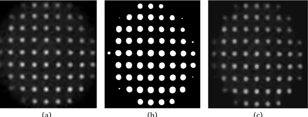
Figure 36 – Example of image analysis of a hartmogram to determine the spot-‐centroid position: (a) hartmogram, (b) binary image and (c) spots marked with a cross. ... 34
Figure 37 – Relation between the local wavefront (WF) aberration W and the ray deviation. ... 34
Figure 38 – A piece of the mold used in the production of the first microlens array for the H-‐S sensor. ... 37
Figure 39 – Illustration of the thermal reflow process to build microlens arrays (DALY, STEVENS, et al., 1990). ... 38
Figure 40 – Bulk micromachining of silicon. ... 39
Figure 41 – Spherical shape formed by anisotropic KOH etching of silicon (DE LIMA MONTEIRO, AKHZAR-‐MEHR, et al., 2003). ... 40
Figure 42 – Frequency spectrum of different microlens arrays. ‘Hex61’ stands for regular hexagonal array; ‘move61’, for hexagonal with small random displacements in the center position of each microlens; and ‘MC61’ stands for random array generated by Monte Carlo simulation. All masks contain 61 microlenses (SOLOVIEV and VDOVIN, 2005). ... 41
Figure 43 – Human eye anatomy (a) and optics (b). ... 44
Figure 44 – Hartmann-‐Shack aberrometer used in ophthalmology. ... 44
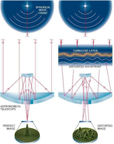
Figure 45 – Illustration of the effect of turbulent atmosphere on astronomical images (HEIN, 2005). ... 46
Figure 46 – AO system (GREENAWAY and BURNETT, 2004). ... 48
Figure 47 – Micromachined membrane deformable mirror (OKO TECHNOLOGIES, 2006). ... 49
Figure 48 – Representation of a reflective surface correcting for wavefront aberration. .... 50
Figure 49 – Astronomical images taken with (right) and without (left) AO (KECK OBSERVATORY; UCLA GALACTIC CENTER GROUP, 2007/2008). ... 51
Figure 50 – Retinal image with (center and rightmost) and without (leftmost) AO for the right eye of a living human subject. The image in the center is just a snapshot while the image on right is an average of 61 frames (ROORDA, 2000). ... 51
Figure 51 – Series of images showing how cones can be imaged in detailed using AO (IMAGINE EYES SA). ... 51
Figure 52 – Objective function for the microlens-‐array optimization. ... 54
Figure 53 – Schematics of the optimization function operation. ... 55
Figure 54 – Block-‐diagram of the Hartmann-‐Shack numerical model. ... 56
Figure 55 – Geometrical representation of the optical system. ... 59
Figure 56 – Steps for calculating the light beam deviation after passing through a plano-‐ convex lens. ... 59
Figure 57 – Zernike coefficients distribution generated by the algorithm. ... 60
Figure 58 – The three types of children in a new generation. ... 63
Figure 59 – Performance of the 10 optimized 10-‐microlens arrays. ... 67
Figure 60 – Optimized 10-‐microlens best array. Units of the axis values are micrometers. ... 68
Figure 61 – Performance of the 10 optimized 16-‐microlens arrays. ... 68
Figure 62 – Optimized 16-‐microlens best array (black diamond) and rectangular 16-‐ microlens array (gray cross). Units of the axis values are micrometers. ... 68
Figure 64 – Optimized 36-‐microlens best array (black diamond) and rectangular 36-‐
microlens array (gray cross). Units of the axis values are micrometers. ... 69
Figure 65 – Comparison of the performance of different microlens-‐array geometries (OLIVEIRA and DE LIMA MONTEIRO, 2011). ... 70
Figure 66 – Maximum number of Zernike terms (or modes) that can be reliably reconstructed for a given number of microlenses using rectangular arrays (YOON, 2006). ... 71
Figure 67 – Influence of rotation of the microlens arrays on the mean reconstruction error for each array. In the legend, the numbers represent the number of microlenses in each array and the letters represent the array geometry: ‘rect’ stands for rectangular and ‘opt’, for optimized. ... 73
Figure 68 – Influence of rotation of the microlens array on the reconstruction error calculated in a set of 2,000 wavefront aberrations. ... 73
Figure 69 – Plane view of Zernike terms. The piston, tip, tilt (not shown) and defocus terms were not taken into account in the optimization. ... 74
Figure 70 – Illustration of the silicon wafer used in the fabrication of the microlens array. ... 75
Figure 71 – Pattern transferred to the photoresist layer. The lateral dimension of the opening is about 10µm. ... 77
Figure 72 – Inverted pyramid formed after KOH etching. ... 77
Figure 73 – Microlens-‐array molds produced. ... 79
Figure 74 – Replication of the microlens arrays: a) UV curing of photopolymer and b) detachment of the cover glass with the optical adhesive. ... 80
Figure 75 – Fabricated microlens arrays. ... 81
Figure 76 – Microlens arrays imaged with SEM. ... 81
Figure 77 – Image generated by the 16-‐microlens rectangular array in the proximity of the focal plane. ... 82
Figure 78 – Schematics of the optical setup for the observing the focusing ability of the array. ... 82
Figure 79 – Optical setup designed to characterize intraocular lenses. ... 83
Figure 80 – Adapted optical setup to test the microlens arrays. ... 83
Figure 81 – Arbitrary wavefront aberration chosen to test the arrays. ... 84
Figure 82 – Hartmograms generated by the fabricated arrays for the arbitrary aberration used. ... 85
Figure 83 – Comparison among the fabricated and the commercial arrays. In the legend, the numbers represent the number of microlenses in each array and the letters represent the array geometry: ‘hex’ stands for hexagonal; ‘opt’, for optimized; and ‘rect’, for rectangular. ... 86
Figure 84 – Comparison of the Zernike coefficients of the 16-‐microlens optimized array (16 opt) and the 127-‐microlens hexagonal array (127 hex). ... 87
Figure 85 – Deviation of the values of the Zernike terms for each array with respect to the values of the 127-‐microlens hexagonal array. The hatched rectangles are used as a reference to identify differences smaller than 0.5λ, 0.25λ and 0.1λ. ... 88
Figure 86 – An example of an output image of the Hartmann-‐Shack method. ... 98
Figure 87 – Block-‐diagram of the image-‐processing algorithm. ... 99
Figure 88 – Graph of the offset function. ... 100
Figure 90 – Detection of light spots. The lateral size of the mask used in the picture on the
right is 20 times bigger than the one on the left. ... 102
Figure 91 – Example of white regions that do not represent light spots. The acquired image is shown in (a) and the binary image, in (b). ... 102
Figure 92 –(a) Acquired image. (b) Image with light-‐spots centroids detected (marked with a small black cross in the middle of a white box). ... 103
Figure 93 – Lenses configuration for optical phase conjugation. ... 105
Figure 94 – AO system design. ... 106
Figure 95 – AO system assembled. ... 107
Figure 96 – (a) Far-‐field and (b) interferogram images without the beam splitter. ... 107
Figure 97 – (a) Far-‐field and (b) interferogram images generated with the beam splitter. ... 108
LIST OF TABLES
Table 1 – Zernike terms. ... 16
Table 2 – Definition of variables to describe the lens model. ... 58
Table 3 – Reconstruction errors generated by optimized and rectangular arrays over 2,000 wavefront aberrations (λ=633nm). ... 69
Table 4 -‐ Condition number and rank of the matrix B!B. ... 72
1.
INTRODUCTION
“If the Theory of making Telescopes could at length be fully brought into Practice, yet there would be certain bounds beyond which telescopes could not perform. For the air through which we look upon the stars, is in a perpetual tremor; as may be seen by the tremulous motion of shadows cast from high towers, and by the twinkling of the fix’d stars. But these stars do not twinkle when viewed through telescopes which have large apertures. For the rays of light which pass through divers parts of the aperture, tremble each of them apart, and by means of their various and sometimes contrary tremors, fall at one and the same time upon different points in the bottom of the eye, and their trembling motions are too quick and confused to be perceived severally. And all these illuminated points constitute one broad lucid point, composed of those many trembling points confusedly and insensibly mixed with one another by very short and swift tremors, and thereby cause the star to appear broader than it is, and without any trembling of the whole. Long telescopes may cause objects to appear brighter and larger than short ones can do, but they cannot be so formed as to take away that confusion of the rays which arises from the tremors of the atmosphere. The only remedy is a most serene and quiet air, such as may perhaps be found on the tops of the highest mountains above the grosser clouds.” (NEWTON, 2007).
When trying to observe fainter astronomical objects (such as other galaxies), using large telescopes, astronomers faced a limitation: images appeared blurred and the objects could not be distinguished. The reason was that light coming from the astronomical object passed through turbulent atmosphere before reaching the telescope lenses (HEIN, 2005). As claimed by Sir Isaac Newton in his Opticks, the “quiet air” of high mountains contributes to better observations. However, even such a “serene air” is prone to contain turbulences, and therefore, to decrease the quality of the observed image by introducing aberrations in the light beam that passes through it.
Despite representing a big problem in fields such as astronomy, communications and defense, it was only in the second half of the 20th century that astronomers and the military started to develop ways of overcoming turbulent effects of the atmosphere. Although it is impossible to avoid the introduction of aberrations in the images when light passes through the atmosphere, it is feasible to compensate for these aberrations, using a deformable element in the optical system. Basically, in practice, the system must be capable of detecting the deformation present in the image, quantifying it and converting the results into information useful to actuate the deformable element. A requirement is that all this has to be continually performed in a loop and in real-‐time. Hence, an optical system like this would constantly adapt itself to the atmospheric turbulence, therefore compensating for the deformations present in the observed images.
Hence, measuring the aberrations is of great importance to find ways of overcoming the problems imposed by them. In ophthalmology, this is done by means of equipment referred to as aberrometers. There are several different methods to measure aberrations both qualitatively and quantitatively, as will be discussed later. The most widely used method is called Hartmann-‐Shack. In this method, the core component is a microlens array, which is responsible for sampling the aberrated light beam into light spots on the focal plane. The positions of the light spots are directly related to the amount of aberration present in the beam. Thus, if these positions are measured, the aberration can be quantified after some computer processing.
The distribution pattern of the microlenses on the array influences on how it samples a given set of aberrations. Therefore, a pattern that is optimized to fit a given aberration statistics provides benefits such as reduction of the measurement error and/or reduction in the necessary processing time to obtain a mathematical description of the aberration.
The objective of this work is to optimize the microlens array to be used in the measurement of ocular aberrations. This is accomplished in basically three steps. First, a numerical method is proposed to find the distribution pattern of the microlenses in the optimized arrays. Second, the resulting arrays are fabricated. At last, they are tested in an
2.
OPTICAL ABERRATIONS
2.1.WAVEFRONTS
An optical aberration can be understood as a distortion in a wavefront introduced by optical components or by the propagating medium. To define it more precisely and to understand how it can affect the image quality, it is important to first introduce the concept of a wavefront.
Let 𝐿 be a light beam travelling from left to right. The electrical field vector associated to
the beam can be written as a combination of specific plane waves (DE LIMA MONTEIRO, 2002; HECHT, 2002). In a general form, the electrical field vector 𝑬 due to an electromagnetic field can be expressed as in equation 1.
𝑬 𝑥,𝑦,𝑧,𝑡 =𝑨(𝑥,𝑦,𝑧,𝑡)∙𝑒!"(!,!,!,!) 1 where 𝑥,𝑦 and 𝑧 are the spatial coordinates, 𝑡 is the time, 𝑨 is the amplitude and 𝜙 is the phase (GREIVENKAMP, 1995).
The hypothetical surfaces for which all the components of the electrical field have the same phase are called optical wavefronts, as illustrated in Figure 1. The wavefront is also sometimes called a phasefront.
Figure 1 – Wavefronts (dashed line) for parallel and spherically divergent light beams.
A connection can be made between geometrical and wave optics, if it is taken into account that the local normal vector to the wavefront corresponds to the propagation direction of the field. Then, a wavefront can also be defined in geometrical optics as a surface that has normal vectors parallel to the light rays.
In other words, an optical wavefront can also be defined as the surface of constant optical path length (OPL) from the source (OPTICAL SOCIETY OF AMERICA, 1994; GREENAWAY and BURNETT, 2004). The OPL is given by:
𝑂𝑃𝐿= 𝑛(𝑠)∙𝑑𝑠 !
!!
2
When the phase pattern of the electrical field of a light beam becomes distorted, the wavefront changes its shape and is hence referred to as aberrated. The distortions introduced to the wavefront can compromise a quality parameter in the information it carries. The altered parameter can be, for instance, intensity, contrast or delay, depending on the information carried being power, image or sequential signal. Often, the aberration itself is the parameter of interest, as it represents an imprint of the medium or object the wavefront has traversed – refracted or reflected, thus providing a contactless method to probe its shape or homogeneity.
2.2.ABERRATIONS
In some cases, it is useful to describe, rather than the wavefront shape, the difference between the actual wavefront and a reference one, which can be the initial or the desired wavefront. Common reference wavefronts1 are the plane and spherical ideal wavefronts.
In this sense, the wavefront aberration 𝑊 can be defined as the optical path length from the reference to the actual wavefront, as illustrated in Figure 2 (YOON, 2003). In this work, the term optical aberration, or simply aberration, is used with the same meaning as the term wavefront aberration.
Figure 2 – Wavefront aberration.
From equation 2, it can be noted that when a wavefront passes through a medium with different refractive indices, the different rays that compose the beam will have different OPL and therefore the wavefront will no longer have the same shape, as shown in Figure 3 (DE LIMA MONTEIRO, 2002). Two parallel plane-‐waves, 𝐴 and 𝐵, go from 𝑎 to 𝑎′ and from 𝑏 to 𝑏!, respectively, through a medium with index of refraction 𝑛 =1. At point 𝑃
!, both waves have the same phase 𝜙!. Between points 𝑃! and 𝑃!, wave 𝐴 passes through a
medium of length 𝐿 and index 𝑛, which introduces a phase delay in the wave. As a consequence, at point 𝑃!, wave 𝐵 has the same phase as wave 𝐴 at point 𝑃!! and wave 𝐴 has the phase 𝜙!. Therefore, at 𝑎′ and 𝑏!, the waves are not in phase, as they were at 𝑎 and 𝑏.
1 Those reference wavefronts are for general optical systems. In ophthalmology, a convenient
Figure 3 – Wavefront aberration introduced by a non-‐isotropic medium.
The fluctuations in the index of refraction through an optical path may occur for many different reasons: thermal fluctuations, gases, fog and turbulence in general.
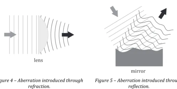
Another situation in which the shape of a wavefront may be altered is when a light beam reaches a non-‐flat optical surface. It can be a surface separating two different transparent media or a reflective surface. In the former case, the aberration is introduced through refraction and, in the latter, through reflection. Figure 4 shows the aberration introduced in a plane wavefront by a lens and Figure 5, by a non-‐flat mirror.
Figure 4 – Aberration introduced through refraction.
Figure 5 – Aberration introduced through reflection.
In the first case, those rays passing through the center of the lens and the ones passing close to the edges will have different OPL, once it depends on the length of the path inside the component, as can be noted from equation 2. It means that an initially plane wavefront will have the shape of the lens surface imprinted on it. The same analysis stands for when the aberration is introduced through reflection. Different regions of the deformed surface of the mirror will alter the OPL of the rays, which compose the beam. Then, a wavefront which was initially plane, for instance, will have the shape of the reflective surface imprinted on it, i.e., the wavefront will become aberrated.
Figure 6 –Aberrated wavefronts after influenced by optical components with the same surface profile: (left) refractive, with refractive index n, and (b) reflective.
Wavefront aberrations vary with the wavelength, once the index of refraction depends on that. When several different wavelengths are present, the aberrations are said to be chromatic. In the case when only one wavelength is taken into account, the aberrations are said to be monochromatic, which is the case of the present work.
The first published systematic treatment of geometrical monochromatic aberrations was due to Seidel, who mathematically described five basic aberrations, which arise from a third-‐order approach of light propagation through real lenses (BORN and WOLF, 1989). The five primary Seidel aberrations are: spherical aberration, coma, astigmatism, curvature of field and distortion. They are described in the next paragraphs.
2.2.1. SPHERICAL ABERRATION
The spherical aberration can be defined as the variation of focal distance with aperture diameter (SMITH, 2007). In the geometrical optics theory, the focal distance of a spherical lens is well defined only if the light beam impinges on a small central region of the lens, what is called the paraxial approximation. Otherwise, the theory predicts a variation on the focal distance according to the position where rays impinge on the lens surface relative to the optical axis2 (BORN and WOLF, 1989). Figure 7 illustrates the spherical aberration
introduced by a simple converging lens3. It happens because rays (𝑅) that impinge on the
periphery of the lens are more deviated than the paraxial rays. Thus, those rays intersect the optical axis (𝑂𝐴) before the paraxial focus (𝐴). The distance (𝐿𝐴’) from the paraxial focus to the axial intersection 𝐵 is called longitudinal spherical aberration. When the spherical aberration is measured on the focal plane (𝐴𝐶), it is called transverse or lateral spherical aberration (𝑇𝐴’).
2 The spherical aberration can be easily observed with spherical lenses. Actually, it depends also on
the lens surface. Theoretically, lenses with refractive index higher than the surrounding media and with hyperbolic surfaces do not introduce any spherical aberration. They are called aspherical lenses.
3 In the present work, it is always assumed that the lens has a larger index of refraction than the one
Figure 7 – The spherical aberration schematics in a spherical lens.
2.2.2. COMA
The coma aberration is due to the dependence of transverse magnification on the aperture diameter (HECHT, 2002; BORN and WOLF, 1989). It is particularly evident when the ray bundle is oblique and the image point is off-‐axis. This is illustrated in Figure 8, where the marginal rays, i.e. the ones that impinge on the periphery of the lens, arrive at the focal plane closer to the axis than the rays in the vicinity of the principal ray, i.e. the one that passes through the lens center. Coma also depends on the lens shape and can therefore be minimized. The shape for which coma is zero for distant objects is nearly convex-‐planar (HECHT, 2002). In practice, when dealing with collimated beams, as is often the case in aberrometry, it is important to guarantee that the beam impinges parallel to the lens optical axis and centered to it.
Figure 8 – Illustration of the coma aberration generated by a spherical lens.
2.2.3. ASTIGMATISM
ophthalmology to compensate for the astigmatism introduced by the cornea (see section 5.1 for a description of the human eye). In a general optical system, this correction can be achieved also with the use of mirrors, also designed with different curvature radii in different perpendicular planes.
Figure 9 – Illustration of astigmatism introduced by a spherical lens.
2.2.4. CURVATURE OF FIELD
The curvature of field, also called Petzval curvature or field of curvature, is an aberration that causes planar objects to appear curved in the image. That means that the focal surface, where the image is generated, is curved instead of plane, as expected by the paraxial theory. In the absence of astigmatism, this surface is a paraboloid and is called the Petzval surface. (HECHT, 2002) This aberration is more evident for off-‐axis images and is illustrated in Figure 10.
Figure 10 – Field of Curvature.
2.2.5. DISTORTION
outwards (barrel) with respect to the optical axis. Figure 11 shows distortion in the image of a square grid. Distortion appears when the image magnification is a function of the off-‐ axis image distance so that the realized position of each image point is different from the predicted one (HECHT, 2002). In general, all lenses introduce some degree of distortion. However, those with strongly curved surfaces present higher levels of distortion. A common and practical technique to reduce distortions in an optical system is to use compound lens system approximately symmetrical about a stop center (CHEN, SU, et al., 2010).
Figure 11 – Distortion aberration: pincushion (on left) and barrel (on right).
2.3.QUANTITATIVE DESCRIPTION OF OPTICAL ABERRATIONS
Once the wavefront aberrations concept is understood, as well as its effects, it is convenient to represent them mathematically. There are two methods by which the wavefront may be represented: zonal estimation4 and modal estimation. According to
Southwell (1980), the latter is superior to the former in terms of error propagation and is also computationally easier and faster. It is the one used in this work.
In the modal estimation, it is assumed that a wavefront can be described by an infinite sum expansion of orthogonal functions (CUBALCHINI, 1979). In other words, the wavefront can be represented by the weighted superposition of orthogonal two-‐dimensional basis functions, also referred to as spatial modes, Zernike modes or Zernike terms.
Commonly the wavefront aberrations are represented by the Zernike polynomials5 (BORN
and WOLF, 1989). Zernike polynomials are a set of polynomials defined on a unit circle and, therefore, can be easily described in polar coordinates as a product of angular functions and radial polynomials. The angular functions are the basis functions for two-‐ dimensional rotation group, and the radial polynomials are derived from Jacobi polynomials (NOLL, 1976).
4 The zonal estimation is a discrete approach to describe the wavefront shape 𝑊 𝑥,𝑦 =𝑧 point by
point in a mesh. It consists in attributing values (𝑧), which represent the surface height, to discrete
mesh points (𝑥,𝑦) in space. The wavefront shape may be visualized by a wire frame connecting all z
points in the three dimensional space.
5 Recently, an alternative orthogonal polynomial basis has been proposed to describe the wavefront
There is no general strict correspondence between Zernike polynomials and Seidel aberrations. When only low-‐order aberrations are considered, spherical aberration, coma and astigmatism can be directly represented by single Zernike terms. Otherwise, aberrations such as distortion and field curvature are represented as a weighted sum of different Zernike terms.
Zernike polynomials are convinient to describe wavefront aberrations because they are orthogonal over a unit circle and most of the optical components, apertures and laser beams are circular. This set of polynomials is often used also because it is made up of terms that are of the same form as the types of aberrations often observed in optical tests (ZERNIKE, 1934 apud WYANT and CREATH, 1992). These terms are linearly independent and represent individually different types of aberrations. Therefore, an aberrated wavefront 𝑊 𝜌,𝜑 may be represented by a sum of Zernike terms 𝑍!(𝜌,𝜑) conveniently weighted through multiplication by coefficients (𝐶!), as shown in equation 3.
𝑊 𝜌,𝜑 = 𝐶!𝑍!(𝜌,𝜑)
!
!!!
3
It is important to emphasize that the Zernike terms are defined with amplitude ranging from −1 to +1 with zero average. The actual amplitude of each term in a real wavefront aberration is determined by the value of the coefficients (𝐶!).
There is no universal standard for Zernike terms indexation (WYANT and CREATH, 1992). Here, 𝑗 is used for single-‐index ordering, which is convenient for numerical purposes. Different authors may however use different indexation standards. A common single-‐ index indexation scheme is proposed by Noll (1976).
Another common way for ordering Zernike terms is to use a double index: 𝑛 and 𝑚. Each of the Zernike polynomials is composed by three components: normalization factor, radial-‐dependent component and azimuthal-‐dependent component. The index 𝑛 describes the highest power (order) of the radial component and 𝑚 describes the azimuthal
frequency of the sinusoidal component (PORTER, QUEENER, et al., 2006).
Thibos et al. (2002) proposes a conversion standard from single-‐ to double-‐index schemes and vice-‐versa, as shown in equations 4 and 5.
𝑗=
𝑛 𝑛+2 +𝑚
2 4
𝑛=𝑟𝑜𝑢𝑛𝑑𝑢𝑝 −
3+ 9+8𝑗
2 𝑚=2𝑗−𝑛(𝑛+2)
5
Zernike polynomials are defined, in polar coordinates, as in equation 6 (BORN and WOLF, 1989).
𝑍! !
𝜌,𝜑 =
𝑅!! 𝜌 cos 𝑚𝜑 , 𝑚>0
𝑅!! 𝜌 sin 𝑚𝜑 , 𝑚<0
𝑅!
!
, 𝑚=0
6
where 𝑛 and 𝑚 are integers, 𝑛 >0, 𝑛≥ 𝑚, 𝑛− 𝑚 is even, 𝜌 is the normalized radial distance, 𝜑 is the azimuthal angle in radians and 𝑅!
!
𝑅! !
𝜌 = −1
! 𝑛
−𝑘 !
𝑘! 𝑛+𝑚
2 −𝑘 !∙
𝑛−𝑚 2 −𝑘 !
(!!!)/!
!!!
𝜌!!!! 7 The polar coordinates 𝜌 and 𝜑 are defined according to Figure 12.
Figure 12 – Polar system coordinates.
The equations for some Zernike terms are show in Table 1. A three-‐dimensional representation for some terms, as well as commonly used names, is shown in Figure 13.
Table 1 – Zernike terms.
𝒋 𝒏 𝒎 𝒁𝒏𝒎 𝝆,𝝋 Name
0 0 0 1 Piston
1 1 -‐1 2𝜌sin (𝜑) y-‐Tilt
2 1 1 2𝜌cos (𝜑) x-‐Tilt (Tip)
3 2 -‐2 6𝜌!sin (2𝜑) Astigmatism 45°
4 2 0 3(2𝜌!−1) Defocus
5 2 2 6𝜌!cos (2𝜑) Astigmatism 0°
6 3 -‐3 8𝜌!sin (3𝜑) Trefoil
7 3 -‐1 8(3𝜌!−2ρ)sin (𝜑) y-‐Coma
8 3 1 8(3𝜌!−2ρ)cos (𝜑) x-‐Coma 9 3 3 8𝜌!cos (3𝜑) Trefoil
The first Zernike term is called piston (𝑛 =0, 𝑚=0) and corresponds to a variation in the
absolute value of the OPL for the whole light beam, i.e., it corresponds to a uniform shift in the whole wavefront along the optical axis. Therefore, the piston term does not represent an aberration, but actually an overall delay, and is generally not taken into account.
Referring to Table 1, the radial orders for 𝑛=1 and 𝑛 =2 are generally referred to as
low-‐order aberration, while the others are called high-‐order aberrations. However, this classification is not standardized and may vary from author to author.
The tilt terms (𝑛=1) affect the wavefront by causing a shift of its center location in the
Therefore, adaptive optics systems often attribute the task of correcting for wavefront horizontal and vertical tilts to a specialized tip-‐tilt control mirror, while the wavefront modulator (see section 5.2) is used to correct for aberrations with radial orders higher than 2 (TYSON, 1999).
Figure 13 – 3D representation of Zernike terms.
The defocus term is commonly dominant in wavefront aberration measurement, especially in ophthalmology where the eye exhibits a considerable dioptric power when compared to the other usually occurring high-‐order eye aberrations. The dioptric power of a lens measures the power to which a lens can bend the propagation direction of light rays. It is defined as the reciprocal of the focal length, in meters, and is given in diopters, in the MKS unit system.
2.4.EFFECTS OF ABERRATIONS ON OPTICAL SYSTEMS
of the system PSF and the object. Therefore, systems with poorly resolved PSF generate images of reduced quality.
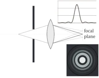
In geometrical optics, a perfect system would generate a point as the image of a point source. However, in practice, even the perfect optical systems are diffraction-‐limited and the image observed for a point source, i.e., the PSF for such systems, is an Airy disc.
In Figure 14, it is illustrated the PSF for a diffraction-‐limited system. When a light beam passes through an aperture or lens, it undergoes the diffraction effect (HECHT, 2002). That means that, for a perfect lens, the observed image at the focal plane consists of a sequence of concentric rings where the center is the brightest region and the outer rings are less intense than the inner ones. The top-‐right inlet graph shows the light intensity distribution over the focal plane.
Figure 14 – Image formation of a point source for a diffraction-‐limited system.
The diffraction-‐limited system illustrated in Figure 14 can be a simplified model of a perfect human eye, for instance, where the lens6 corresponds to the eye compound lens
system (cornea and crystalline lens – see section 5.1 for a description of the human eye), and the focal plane corresponds to the retina.
Perfect systems, such as the ideal simplified model of the human eye, generate diffraction-‐ limited images, once they do not introduce any aberration in the incoming wavefront. When the system is aberrated, i.e., when it introduces aberrations in the light beam, the PSF becomes distorted. This is illustrated below by comparing the PSF for a perfect eye (Figure 15) and for an emmetropic eye (Figure 16). In both figures, the PSF is shown for different pupil diameters, ranging from 1 to 7 mm. The pupil diameter refers to the
diameter effectively used with the lens and the smaller it is, the larger the disc diameter at the focal plane.
The PSFs for an emmetropic eye demonstrate the effect of aberrations in the image of a point source to be observed at the retina. These aberrations are introduced mainly by the cornea and crystalline lens of the eye. It can be noted that the larger the pupil diameter,