Stringent limits on top-quark compositeness from
t
¯
t
production at the
Tevatron and the LHC
M. Fabbrichesi,1 M. Pinamonti,2 and A. Tonero3 1Sezione di Trieste, INFN, 34136 Trieste, Italy 2
Gruppo collegato di Udine, Sezione di Trieste, INFN and SISSA, via Bonomea 265, 34136 Trieste, Italy 3ICTP South American Institute for Fundamental Research & Instituto de Física Teórica,
UNESP, Rua Dr. Bento T. Ferraz 271, 01140-070 São Paulo, São Paulo, Brazil (Received 19 September 2013; published 11 April 2014)
If the top quark is a composite state made out of some constituents, then its interaction with the gluon will be modified. We introduce the leading effective operators that contribute to the radius and anomalous magnetic moment of the top quark and study their effect on the cross section for t¯tproduction at the Tevatron and the LHC. Current measurements of the cross sections set a stringent limit on the scale of compositeness. This limit is comparable to similar limits obtained for light quarks and those from electroweak precision measurements. It can be used to constrain the parameter space of some composite Higgs models.
DOI:10.1103/PhysRevD.89.074028 PACS numbers: 14.65.Ha, 12.60.Rc, 13.85.Lg
I. MOTIVATIONS
Whether the top quark is a point-like particle or an extended object is a question that can now be addressed thanks to the large number of them produced at the LHC and the Tevatron. The most recent, combined measurement of the cross section fort¯tproduction is in good agreement with the most up-to-date theoretical prediction within the standard model (SM) and this result can be used to put constraints on the compositeness of the top quark.
Whereas in the SM the top quark—as well as all other fundamental particles—has no structure, various extensions of the SM are based on some form of compositeness: in particular, the composite Higgs boson[1,2], as well as its partial compositeness implementation[3,4], but also mod-els inspired by the littlest Higgs [5] and technicolor [6] assume the existence of a strongly interacting sector, the SM particles being either composite objects themselves or mixing with particles which are. The top quark, being the heaviest of all states, is the best candidate for searching for possible signatures of such compositeness. The problem has been previously addressed in[7]and more recently in [8–15]. We discuss in some detail the implications of the
limits we find on possible extensions to the SM in the last section.
A. Composite top quark and strong interactions Compositeness can manifest itself in various ways. We take the most direct approach and look into what effect a finite extension of the top quark has on its interaction with the gauge bosons. In the case most relevant for collider physics, we can write two form factorsF1ðq2Þ andF2ðq2Þmodifying the vertex between the top quark and the gluon as
gs¯t
γμF 1ðq2Þ þ
iσμνq ν 2mt
F2ðq2Þ
Gμt; (1)
where gs is the strong SUð3ÞC coupling constant, Gμ¼ TAGAμ is the gluon field, TA are the SUð3ÞC group generators, qμ is the momentum carried by the gluon, t denotes the top-quark field and σμν¼i½γμ;γν=2. The interaction in eq.(1)is the most general after assuming that the vector-like nature of the gluon-top–quark vertex is preserved by the underlying dynamics giving rise to the composite state.
As originally pointed out for the case of electromagnetic interactions[16], the physics of the form factors in eq.(1) is best represented by the combinations
GEðq2Þ ¼F1ðq2Þ þ q2 4m2
t
F2ðq2Þ and
GMðq2Þ ¼F1ðq2Þ þF2ðq2Þ; (2)
which are (in the Breit frame) the Fourier transform of, respectively, the chromoelectric and chromomagnetic charge densitiesρc andμρm of, in our case, the top quark. For an extended object these densities are not Dirac
δ-functions and can be expanded. To the leading order, we thus obtain a first momentum (the chromomagnetic momentμ),
GMðq2Þ ¼ 2 π
Z
drr2j
0ðqrÞμρmðrÞ≃μþ ; (3)
GEðq2Þ ¼2 π
Z
drr2j
0ðqrÞρcðrÞ≃1− ~q2
6 h~r
2i þ ; (4)
from the chromoelectric charge density. In Eqs. (3)–(4), j0ðxÞ ¼sinx=xrepresents the spherical Bessel function of order zero and the (nonrelativistic) chargesρc andρm are related to the four-current as
jμðrÞ ¼ ðg
sρcðrÞ;μ~σ×∇~ρmðrÞÞ: (5)
The two parameters μ and h~r2i are traditionally used in nuclear physics to characterize the finite extension of nucleons and other extended objects.
Form factors are just a way of organizing the perturbative expansion. An alternative and perhaps better approach is effective field theory. In this language the expansion is given in terms of operators invariant under the underlying symmetries that are added to the SM Lagrangian. These operators have a dimension higher than four and are suppressed by negative powers of the new physics scale to get the required dimension.
In this work we use the effective field theory approach and consider the contributions given bySUð3ÞC×Uð1Þem invariant effective operators to the top-quark form factors introduced in eq.(1). The leading contributions come from the following two higher dimensional operators:
ˆ O1¼gs
C1 m2 t ¯ tγμT
AtDνGAμν and
ˆ O2¼gs
C2υ 2m2 t ¯ tσμνT
AtGAμν; (6)
where DνGA
μν ¼∂νGAμνþgsfABCGνBGCμν, GAμν¼∂μGAν− ∂νGA
μþgsfABCGBμGCν is the gluon field strength tensor, fA
BCare theSUð3ÞCstructure constants andυ¼174GeV is the electroweak (EW) symmetry breaking vacuum expectation value. In eq. (6) the operators Oˆ1 and Oˆ2 are, respectively, of the dimension six and five. We limit ourselves to theCP-conserving case and the dimensionless coefficientsC1andC2are taken to be real. Left- and right-hand fermion fields enter symmetrically. The operatorOˆ1 gives the leadingq2 dependence toF
1whileOˆ2gives the q2-independent term ofF
2:
F1ðq2Þ ¼1þC1 q2 m2
tþ
… and F2ð0Þ ¼2C2 υ
mt : (7)
Operators of higher dimensions can in general contribute—they give further terms in the expansion of the form factors—but their effect should be suppressed. We have checked that possible corrections due to dimension eight operators, such as
GμνGμνq¯H t~ R; (8)
are suppressed as long as the coefficients are taken to be OðC2
1;2Þ.
The form of the coefficients in front of the operators in eq. (6) is conventional and dictated, in our case, by the analogy with the electromagnetic form factors. In addition, the operator Oˆ2 is written for convenience with an extra factor υ=mt because it can be thought as coming, after EW symmetry breaking, from a dimension sixSUð3ÞC× SUð2ÞL×Uð1ÞY gauge invariant operator that includes the Higgs boson field.
Replacing the expressions of the form factors obtained in eq.(7)into eq.(2), we can obtain an estimate of the radius and chromomagnetic moment of the top quark using the same formulas that apply in the electromagnetic case. We have that
h~r2i ¼−6dGE d~q2
q2¼0
and μ¼GMð0Þ; (9)
whereμ is the chromomagnetic moment of the top quark measured in units ofgs=2mt.
The aim of this work is to give an estimate of the size of these quantities by constraining the values of the dimen-sionless coefficients C1 and C2 using the available LHC public data on thet¯ttotal production cross sectionσðpp→ ¯
ttÞ and those for the σðpp¯ →¯ttÞ from the Tevatron. In addition, we also include constraints from data on spin correlations of the top quarks at the LHC. The results will be used in the last section where we will translate the bounds onC1andC2into limits on new physics scales in the framework of some specific models.
The finite extension of the source generating the terms in eq. (9) arises because of the radiative corrections of the parton-level processes as well as because of the presumed compositeness. In order to disentangle these two contri-butions we assume that the former is included in the SM cross section computed at the next-to-leading order (NLO) and beyond [for the most recent exact computation at the leading order (NNLO) and next-to-next-to-leading logs (NNLL), see [17] and citations therein], leaving C1 and C2 to encode only effects intrinsically due to compositeness.
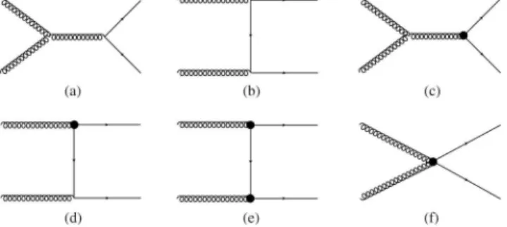
The operators Oˆ1 and Oˆ2 enter at tree level into the computation of the t¯t production cross section through gluon fusion and quark-antiquark annihilation. The first channel is the dominant one at the LHC while the second is dominant at the Tevatron. At tree level, in addition to the usual SM QCD Feynman diagrams, one has to take into account the contributions coming from the new interactions as depicted in Fig.1and Fig.2. The diagram (f) of Fig.1is a contribution not present in the SM and is due to the presence of the operators Oˆ1 and Oˆ2; it represents the effective interaction of two gluons and the¯tt pair. Notice that the contribution of the operatorOˆ1cancels out in the sum of the gluon fusion amplitudes.
Following the effective field theory approach, one has to write down all possible dimension five and six operators that contribute to the t¯t production cross section. It is possible to show [18] that—by rearrangement and field redefinitions using the equations of motion—out of all possible operators that contribute to this process only three are independent, namelyOˆ1,Oˆ2in eq.(6)and a set of four-fermion operators. If we further assume the same coef-ficient in front of the four-fermion operators involving two top quarks and two light quarks of different flavors, then these four-fermion operators too can be rewritten, by means of the equations of motion, in terms of the operator Oˆ1. We are thus left with just the two operatorsOˆ1 andOˆ2in eq.(6). Notice that in general, the whole set of four-fermion operators entering in the dimension six SM effective Lagrangian is larger and cannot be rewritten as O1.
Anomalous couplings and top-quark production has been discussed by several authors [11], most recently in [12](and[13], which came out while we were finishing this work). The anomalous magnetic moment of these refer-ences corresponds to the coefficient C2 of the chromo-magnetic operator in eq.(6). Ref.[14]follows an approach similar to ours but with different and less stringent results. The effect on¯tt-production ofOˆ2(together with the four-fermion operators) has been studied in[15]in the context of nonresonant new physics at the Tevatron and the LHC. See [19]for an updated version.
In the low-energy regime, data on B-physics can be affected by the operators in eq. (6). In particular, the operator O2 contributes to the matching condition of the Wilson coefficient of the chromomagnetic operator
between the quarkbands. The latter operator mixes with the electromagnetic dipole moment operator
embb¯σμνð1þγ5ÞsFμν; (10)
which gives rise to the transitionb→sγ. Even though data on the branching fraction[20]can in principle be used to set limits on the coefficientC2, the estimates in literature give either too small an effect[21]or one with large uncertain-ties [22]. For this reason, we do not use these limits.
II. METHODS
A. Monte Carlo implementation
In order to study new physics effects ont¯tproduction cross sections (and spin correlations) at the LHC and Tevatron, we have first used FEYNRULES[23]to implement our model, which has been defined to be the SM with the addition of the two effective operatorsOˆ1andOˆ2of eq.(6). FEYNRULES provides the universal FeynRules output (UFO) with the Feynman rules of the model. The UFO is then used by MADGRAPH5[24](MG5) to compute the production cross section that we denote byσMG5ðC1; C2Þ. The main t¯t production channel at LHC is given by gluon fusion and the associated Feynman diagrams are those in Fig. 1. Other subleading channels are given by quark-antiquark annihilation, whose diagrams are depicted in Fig.2. MG5 computes the square of the amplitude for each single channel and then convolutes the result with the probability distribution functions (pdf) of the partons inside the proton in order to obtain the totalpp→t¯tproduction cross section. The default set of pdf used is CTEQ6L1.
The partonic level result thus obtained can be compared with the partonic experimental cross section that is extracted by the experimental collaborations from the fully hadronized cross section—which is what is actually mea-sured at the colliders.
We compute, using MG5,σMG5ðC1; C2Þfor three differ-ent values of the cdiffer-enter-of-mass energy (7, 8 and 14 TeV), varying the absolute values of bothC1andC2 in a range that goes from 0 to 0.1. These different values of
σMG5ðC1; C2Þ will be used to obtain limits on the coef-ficients C1 and C2 by comparing the MG5 computation with the measured cross section at the center-of-mass (CM) energy ffiffiffi
s
p
¼7 and 8 TeV and the expected result at 14 TeV, as discussed in the next section.
By proceeding in the same way, we have also computed the t¯t production cross section at the Tevatron and com-pared it with the measured cross section at the CM energy
ffiffiffi
s
p
¼1.98TeV. In this case, the main t¯t production channel is given by quark-antiquark annihilation and the associated Feynman diagrams are those depicted in Fig.2. As we shall see, in this case we obtain a particular stringent bound onC1.
(g) (h)
FIG. 2. Parton-level Feynman diagrams for the process
B. Statistical analysis
The quantity used to obtain 95% confidence level (C.L.) limits on the coefficients C1 and C2 is the cross section
Δσexp, which is defined to be the difference between the central value of the measured cross sectionσ¯expand that of the SM theoretical valueσ¯th:
Δσexp¼σ¯exp−σ¯th: (11)
The uncertainty is given by summing in quadrature the respective uncertainties:
ffiffiffiffiffiffiffiffiffiffiffiffiffiffiffiffiffiffiffiffiffiffiffiffiffiffiffiffiffiffiffiffiffiffiffi ðδσexpÞ2þ ðδσthÞ2
q
: (12)
Using the cross sections σMG5ðC1; C2Þ calculated with MG5, we compute the value of the cross section coming from new physicsΔσMG5ðC1; C2Þas
ΔσMG5ðC1; C2Þ ¼σMG5ðC1; C2Þ−σMG5ð0;0Þ: (13)
The quantityΔσMG5ðC1; C2Þrepresents the contribution to the cross section coming from the interference between the SM leading order and new physics diagrams. Terms coming from the interference between new physics and higher order QCD diagrams are not included in this approximation.
Values ofC1 andC2for which ΔσMG5ðC1; C2Þis more than two standard deviations fromΔσexp, namely
ΔσMG5ðC1; C2Þ>Δσexpþ2
ffiffiffiffiffiffiffiffiffiffiffiffiffiffiffiffiffiffiffiffiffiffiffiffiffiffiffiffiffiffiffiffiffiffiffi ðδσexpÞ2þ ðδσthÞ2
q
; (14)
or
ΔσMG5ðC1; C2Þ<Δσexp−2
ffiffiffiffiffiffiffiffiffiffiffiffiffiffiffiffiffiffiffiffiffiffiffiffiffiffiffiffiffiffiffiffiffiffiffi ðδσexpÞ2þ ðδσ
thÞ2
q
; (15)
can be considered excluded at 95% C.L.
III. RESULTS A. SM cross section
A typical one-loop radiative correction to the vertices gives a contribution to the top-quark radius Oðαs=2πm2tÞ.
Because the effect of compositeness is of the same order, the SM theoretical amplitude σth used for obtaining the exclusion limits, as explained in the previous section, must contain at least NLO contributions which include these corrections as well as those coming from initial and final state radiation.
Production of top-quark pairs at hadron colliders is a challenging computation that has been pursued for many years and is now available at the NNLO[17]. In addition, the soft gluon re-summation for the same process is known at the NNLL order necessary for the matching [25]. Following [17] we take, for a top-quark mass of 172.5 GeV, the following values for the cross section at the LHC for, respectively, the CM energy ffiffiffi
s
p
¼7 and 8:
σthðpp→t¯tÞ
¼
176.25þ4.6
−5.9ðscaleÞþ 4.8
−4.9ðpdfÞpbðLHC@7Þ 251.68þ−8.66.4ðscaleÞ−þ6.56.3ðpdfÞpbðLHC@8Þ
; (16)
where the first uncertainty is due to the residual scale dependence and the second to the pdf of the partons which are taken from the MSTW200NNLO68CL set [26]. At the Tevatron, for a CM energy pffiffiffis
¼1.98TeV, the same reference[17] gives
σthðpp¯ →t¯tÞ ¼7.35þ−0.210.11ðscaleÞþ 0.17
−0.12ðpdfÞpbðTevatronÞ: (17)
The size of the overall uncertainty of these results— summing the square of the two errors—is a substantial improvement with respect to the NLO result.
B. Current data and bounds: LHC and Tevatron The cross section for the production of top-quark pairs has been measured at LHC and Tevatron for its respective energy range.
The best current measurements at the LHC of the cross section σexpðpp→¯ttÞ combining the various channels at the CM energy ofpffiffiffis
¼7TeV, for a top-quark mass of 172.5 GeV, is
σexpðpp→t¯tÞ ¼
177.03ðstatÞ−þ78ðsystÞ 7ðlumiÞpbðATLASÞ
165.82.2ðstatÞ 10.6ðsystÞ 7.8ðlumiÞpbðCMSÞ (18)
for, respectively, the ATLAS [27]and the CMS[28]. A combination of ATLAS and CMS results is available [29] for an integrated luminosity of up to 1.1fb−1:
σexpðpp→¯ttÞ ¼173.310.1pbðLHC@7Þ; (19)
with an overall uncertainty of 5.8% which we will use in our analysis to set the limits.
Figure3 show the limits coming from LHC@7 on the coefficients C1 and C2 obtained by means of the above experimental result and the theoretical computation in eq. (16).
In Fig.3, as well as in the following figures, the black line with dots represents the cross section ΔσMG5 which includes the contributions of the operatorsOˆ1andOˆ2. The yellow (green) bands represent the cross sectionΔσexpwith
its error at the2ð1Þσlevel. Finally, the horizontal red lines represent the expected limits (at the 1 and2σlevels) which are obtained by identifying the central value of the experimental data σ¯exp with the central value of the theoretical predictionσ¯th.
The best current measurements of the cross section
σexpðpp→¯ttÞ at the CM energy of pffiffiffis¼8TeV for a top-quark mass of 172.5 GeV is
σexpðpp→t¯tÞ ¼
237
1.7ðstatÞ 7.4ðsystÞ 7.4ðlumiÞ 4.0ðbeam energyÞpbðATLASÞ
2273ðstatÞ 11ðsystÞ 10ðlumiÞpbðCMSÞ (20) FIG. 3 (color online). Constraints on the coefficientsC1andC2from data at the LHC at
ffiffiffi
s p
¼7TeV. On the left is the limit onC1 withC2¼0. On the right is the limit onC2withC1¼0. The horizontal dashed black line represents the experimental central value. The yellow (green) band represents2ð1Þσuncertainties. The red lines are the expected limits at 1 and2σlevel. The thick black line is the cross section in the presence of the new operators at sampled values of the coefficientsCi.
for, respectively, an integrated luminosity of 5.8fb−1 at ATLAS [30] and 2.4fb−1 at CMS [31], in both cases considering events with dilepton final states.
Lacking a combined value, we consider the experi-mental value of ATLAS [30], which has smaller uncer-tainties, to set the limits; the theoretical value is taken from eq. (16). Figure 4 shows the result in this case. Notice that improved limits with respect to the previous ones at pffiffiffis
¼7 TeV are mainly due to the lower central value of the experimental data. This is made clear by the comparison with the expected C.L. (the red horizontal lines in Fig. 4).
Combined data from CDF and D0 at the Tevatron[32] give the following cross section at the CM energy ofpffiffiffis
¼ 1.96TeV up to an integrated luminosity of 8.8fb−1:
σexpðpp¯ →¯ttÞ ¼7.650.42pbðTevatronÞ: (21)
Figure 5 shows the limits coming from Tevatron on the coefficientsC1 andC2 we obtain by means of the above experimental result and the theoretical computation in eq. (17). The data from the Tevatron are particularly stringent in the case of the operator Oˆ1 because of the FIG. 5 (color online). Constraints on the coefficientsC1andC2from data at the Tevatron at
ffiffiffi
s p
¼1.96TeV. On the left is the limit on
C1withC2¼0. On the right is the limit onC2withC1¼0. The horizontal dashed black line represents the experimental central value. The yellow (green) band represents2ð1Þσuncertainties. The red lines are the expected limits at the 1 and2σlevels. The black line is the cross section in the presence of the new operators at sampled values of the coefficientsCi.
FIG. 6 (color online). Possible constraints on the coefficientsC1andC2from data at the LHC atpffiffiffis¼14TeV. On the left is the limit onC1withC2¼0. On the right is the limit onC2withC1¼0. The horizontal dashed red line represents the experimental central value. The other red lines are the expected limits at the 1 and2σlevels. The black line is the cross section in the presence of the new operators at sampled values of the coefficientsCi.
kinematical configuration that prefers theqq→t¯tchannel which is, in turn, most sensitive to that operator.
C. Future bounds: LHC at ffiffi
s
p
¼14TeV
If we assume that the experimental uncertainty will remain around 5%—it is difficult to imagine doing better than this—we can plot the expected limits at the LHC when the CM energy will be pffiffiffis
¼14TeV by fixing the experimental central value to coincide with the theoretical cross section:
σthðpp¯ →t¯tÞ ¼953.6þ−22.733.9ðscaleÞþ 16.2
−17.8ðpdfÞpb
×ðLHC@14Þ ½17: (22)
As depicted in Fig.6, the increase in energy improves the limits with respect to what was to be expected at the LHC at lower CM energies. However, the study at 14 TeV does not modify in a significative manner the overall limits because the actual experimental value at 8 TeV turned out lower than the theoretical value and therefore yielded a better than expected limit.
D. Differential cross section
Even though the differential cross section for t¯t pro-duction contains, in principle, extra information that can be used to set limits on the compositeness of the top quark, we find that the current experimental uncertainties are too large to significantly improve the best limits we found by considering the total cross section.
The best case occurs for the cross section as a function of the invariant mass mt¯t for the LHC with data at pffiffiffis¼ 7TeV[33]and for the coefficient C1. Figure7 plots this cross section in bins and shows the experimental value with its error and the variation for different values of the coefficientC1.
To set limits combining the total cross sectionσtot¼σt¯t and the relative differential cross section σdif;i¼
ð1=σt¯tÞdσt¯t=dmt¯t in each bin i, we evaluated an χ2 function as
χ2¼
σexptot −σth tot δðσtotÞ
2
þX
Nbins
i¼0
σexp
dif;i−σthdif;i
δðσdif;iÞ
2
; (23)
whereδðσÞrefers to the squared sum of the experimental and the theoretical uncertainties on the respectiveσtot and σdif;i, and the suffix th refer to the theoretical prediction. This theoretical prediction is given by the NLOþNLL calculation [34] plus the contribution from new physics depending on the value ofC1, evaluating generating events with MADGRAPHand then PYTHIA[35].
This quantityχ2is evaluated for each of the considered values ofC1and compared with a distribution ofχ2values obtained generating 103 pseudoexperiments allowing the measured values to fluctuate following a Gaussian distri-butionGðσ;δðσÞÞ. A value ofC1was considered excluded at 95% C.L. if less than 5% of the pseudoexperiments resulted in anχ2 value larger than the one for the given value ofC1.
To get an approximate 95% C.L. exclusion limit onC1, the obtained values of χ2 as a function of C1 were interpolated as shown on the right side of Fig. 7. The dashed horizontal line represents the value χˆ2 for which χ2<χˆ2 in 95% of the pseudoexperiments. The limit we find isC1<0.03, which is an improvement with respect to what was found from data on the LHC total cross section at the same CM energy, but still less stringent than that found from the Tevatron data for the total cross section.
Direct analysis of the Tevatron data[36]and the LHC at
ffiffiffi
s
p
¼8TeV [37] yields weaker limits. The effect of the coefficient C2 on the cross section distributions is negli-gible because of the experimental uncertainties in the different intervals ofmt¯t.
FIG. 7 (color online). Left side: Differential cross section in bins ofmt¯tfor LHC at 7 TeV. In the first bin is the total cross section. In
E. Spin correlations: LHC at ffiffi
s
p
¼7TeV
Independent observables useful in setting further limits on the top-quark structure involve spin correlation in t¯t events[38]. Spin correlations of pair-produced top quarks can be extracted by analyzing the angular distributions of the top-quark decay products in t→Wb followed by the leptonic decay of theW bosonW →lν. If no acceptance cuts are applied and the spin-analyzing power is effectively 100%, then we have the following form of the double angular distribution[38]:
1 σ
d2σ
dcosθ1dcosθ2¼ 1
4ð1þB1cosθ1þB2cosθ2
−Chcosθ1cosθ2Þ; (24)
where B1, B2 andCh are coefficients.
Here, we consider the angular distribution in the helicity basis, in which the quantization axes are taken to be the t and¯t directions of flight in thet¯tzero-momentum frame. Therefore, θ1ðθ2Þ represents the angle between the direc-tion of flight oflþðl−
Þ in thetð¯tÞrest frame and the tð¯tÞ direction of flight in thet¯tzero-momentum frame. In this case the spin correlation coefficientCh is given by
Ch¼
Nð↑↑Þ þNð↓↓Þ−Nð↓↑Þ−Nð↑↓Þ
Nð↑↑Þ þNð↓↓Þ þNð↓↑Þ þNð↑↓Þ; (25)
where Nð↑↑Þ þNð↓↓Þ represents the number of events where the top and antitop-quark spin projections are parallel, and Nð↓↑Þ þNð↑↓Þ is the number of events where they are antiparallel with respect to the chosen quantization axes.
For the experimental analysis it is more convenient to use the one-dimensional distributions of the product
of the cosinesOh≡cosθ1· cosθ2and define an asymme-try Ah which, in the absence of acceptance cuts, is determined by[38]
Ah ¼
NðOh>0Þ−NðOh<0Þ NðOh>0Þ þNðOh<0Þ¼
−Ch
4 : (26)
The most precise experimental measurement of Ch at LHC is obtained by ATLAS studying atpffiffiffis
¼7TeV the angular separation Δϕ between the charged leptons in dileptonict¯t events [39]:
Cmeas
h ¼0.370.06ðstatþsystÞ: (27)
This value has to be compared with the next-to-leading order SM prediction
CNLO
h ¼0.31; (28)
calculated in[38]including QCD and electroweak correc-tions tot¯t production and decay.
The spin correlation coefficientCh as a function of the effective operators coefficients is obtained by means of MG5, generating 105 events for the process pp
→t¯t→ blþνb¯l−ν¯, for different values ofC
1andC2, and computing the asymmetryAhdefined in eq.(26).
MG5 gives a tree level prediction for the total cross section σðpp→t¯t→blþνb¯l−ν¯Þ that we denote by
σMG5ðC1; C2Þ and therefore also the derived asymmetry is a LO result that we denote byAMG5
h ðC1; C2Þ. The tree level prediction for the asymmetry is then corrected in order to take into account the SM NLO effects by computing
FIG. 8 (color online). Constraints on the coefficientsC1andC2from data on spin correlations at the LHC atpffiffiffis¼7TeV. On the left is the limit onC1withC2¼0. On the right is the limit onC2withC1¼0. The horizontal dashed black line represents the experimental central value. The yellow (green) band represents2ð1Þσuncertainties. The red lines are the expected limits at the 1 and2σlevels. The black line is the asymmetryCh computed in the presence of the new operators as a function of the coefficientsCi.
AhðC1; C2Þ ¼ ANLO
h ·σNLOþAMG5h ðC1; C2Þ·σMG5ðC1; C2Þ−AMG5h ð0;0Þ·σMG5ð0;0Þ
σNLOþσMG5ðC
1; C2Þ−σMG5ð0;0Þ
; (29)
where σNLO is obtained by multiplying the NNLO theo-retical cross section fort¯tproduction in[17]by the leptonic decay branching ratio andANLO
h is computed using Eq.(26) from Eq.(28).
Figure8shows the limits on the coefficientsC1andC2 coming from the spin correlations at the LHC at
ffiffiffi
s
p
¼7TeV. The black line represents the correlation coefficient computed including the contributions of the operators Oˆ1 and Oˆ2 as described above. The yellow (green) bands represent the measuredCh with its error at the2ð1Þσlevel. We can see from Fig.8that differently to C1, the coefficientC2 is unbounded for positive values.
F. Combined limits
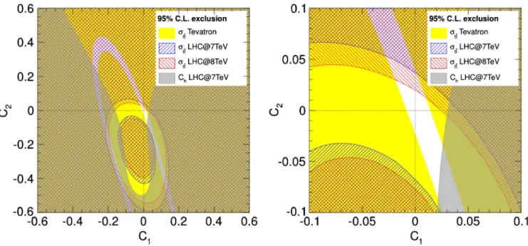
The bounds on the individual coefficientsC1andC2can also be computed when both operators are simultaneously present. In this case, there is an important modulation in the effect of the new operators. The combined limits coming
from the data at the LHC at the two CM energies considered and those at the Tevatron are shown in Fig.9. In the same plot, also the limits coming from the spin correlations are shown.
We can see that without the data on the spin correlations the allowed region is rather large. Other analyses[11–15]
found a smaller region because they either kept only the leading order contribution of the operators or did not combine the limits onC2with those onC1. When the full contribution of these operators is included for both of them, we need the limits from data on the spin correlations in order to exclude the larger values and obtain relevant limits.
IV. DISCUSSION
We have collected in Table I the limits for the two coefficientsC1andC2when they are varied simultaneously and independently of each other for each of the data sets. Pending results from the LHC at pffiffiffis
¼14TeV, the FIG. 9 (color online). Combined limits on the coefficients C1 and C2 from data at the LHC (
ffiffiffi
s p
¼8and 7 TeV) and Tevatron (pffiffiffis
¼1.96TeV). Values in the regions, respectively, in hatched blue and hatched red from LHC, yellow from Tevatron and gray from spin correlations at the LHC are excluded at 95% C.L. The allowed region corresponds to the white area. On the right is a zoomed plot around the allowed values.
TABLE I. Limits on the coefficientsC1andC2when they are varied independently of each other and simultaneously (last column). The starred numbers for LHC@14 are the expected limits.
Tevatron LHC@7 LHC@8 LHC@14 Combined
−0.008≤C1≤0.015 −0.193≤C1≤0.042 −0.165≤C1≤0.025 −0.135⋆≤C
Tevatron gives the most stringent bound on the operatorOˆ1. The LHC at pffiffiffis
¼8TeV and the Tevatron give the best bounds on the operator Oˆ2. In combining the limits, all data sets are important and those from spin correlations are essential in removing large values for the coefficients C1 andC2 which cannot be ruled out by the total cross section data because of cancellations between the two contributions.
A. The size of the top quark
Deviations from the point-like behavior of a particle are usually expressed in terms of charge radius and anomalous magnetic moment. These quantities have been defined in Eq.(3)and Eq.(4). In the case of the top quark the dominant probe is charged under the SUð3Þ group of strong inter-actions. Since there is no definite boundary, the size is usually discussed in terms of the root-mean-squared (RMS) radius. We should first identify the size that comes from radiative corrections. This part is a departure from the point-like behavior due to the cloud of virtual states surrounding any particle in quantum field theory. For the top quark, the leading radiative contribution to the squared mean radius can be computed in perturbation theory to the one-loop order in QCD and it is in general of the order
ðαs=2πÞ1=m2t. Accordingly, this contribution to the RMS radius is about10−5 fm. EW interactions give an additional (smaller) contribution which can be neglected.
We can obtain an estimate of the fraction of the radius and moment of the composite top quark which is not part of the radiative corrections in terms of the effective operator coefficients. Using the formulas in Eq.(7)to compute the form factors of Eq.(2), we have that, using Eq.(9),
h~r2
i ¼644mtC1mþ32υC2 t
and μ¼1þ2 υ mt
C2; (30)
with 2υC2=mt equal to the anomalous component of the magnetic moment. The best constraints on the coeficients C1 andC2when taken independently,
−0.008≤C1≤0.015 and −0.023≤C2≤0.020;
(31)
correspond to a RMS radius,
ffiffiffiffiffiffiffiffi h~r2i
q
<4.6×10⁻⁴fm ð95%C:L:Þ; (32)
and an anomalous magnetic moment,
−0.046<μ−1<0.040 ð95%C:L:Þ: (33)
A similar bound on the anomalous magnetic moment of the top quark has been reported in[12]. The bounds found in [14] are weaker. At the time of writing this paper, an apparently stronger bound was found in [13] which however agrees with our limit if taken at the 68% C.L.
These limits become weaker if the constraints are taken simultaneously for the two operators:
ffiffiffiffiffiffiffiffi h~r2
i q
<7.4×10⁻⁴fm and
−0.17<μ−1<0.062 ð95%C:L:Þ: (34)
To put the above limits in perspective, let us consider the proton and the electron as the best known examples of, respectively, a composite and (presumably) point-like particle. The radiative part of the proton RMS radius is about 10−2fm. Its actual size, as measured in electron-proton elastic scattering experiments, is much larger: it is about 0.9 fm [40]. The factor of 100 in the ratio of these two numbers is not far from what we have found in the case of the top quark.
The electron, which is believed to be a point-like particle, has a limit on its RMS which does not originate in radiative corrections and that is not far from that in Eq.(32)for the top quark: it is10−5fm[41]. In other words, the top quark does not seem to deviate from a point-like object down to a scale close to that of the electron. Notice that the bound in the electron case comes from an analysis ofeþe−
→eþe− while in our case that for the top quark comes fromqq¯ →¯tt rather than the more direct¯tt→¯ttwhich would be probed by the process with four top quarks in the final states. The limit on the part of the electron anomalous magnetic moment not accounted for by radiative corrections is very strong—because of its interaction with a classical magnetic field—and equal to 10
−12 [42].
B. Compositeness and physics beyond the SM The most direct way to associate some compositeness scalesΛ1andΛ2to the effect of the operators in Eq.(6)is through the identification
1 Λ2
1
¼gsmjC21j t
and 1 Λ2
2
¼gsjC2j 2m2
t
: (35)
The identification ofΛ2in Eq.(35)is based on the full EW symmetry group for which the operator Oˆ2 must be considered of dimension six. In this way, it is simple to translate the bounds onC1andC2, obtained in the previous section, into limits on these two scales of compositeness. We have that
Λ1>
8
> <
> :
1.3TeV ðTevatronÞ
0.4TeV ðLHC@7Þ
0.4TeV ðLHC@8Þ
Λ2>
8
> <
> :
1.1TeV ðTevatronÞ
0.9TeV ðLHC@7Þ
0.8TeV ðLHC@8Þ
These results can be compared with bounds coming from EW precision measurements [43]: the scale of the four-fermion operators (for light quarks) is bounded to values higher, depending on the sign and the procedure, than 6.6 or 9.5 TeV. More generally, by using various other operators an the overall bound of Λ>17TeV is found.
While the above identification of the compositeness scale is straightforward—it plays the role of expansion parameter for the operators—its link to specific models is more indirect.
In the following sections we discuss how to translate bounds onC1andC2into limits on the parameters of two models of physics beyond the SM. In doing so, we must bear in mind that often numerical values, when used within a given model, are more orders of magnitude than precise numbers because both naive power counting and the QCD analogy may not be correct in a generic strongly interacting theory.
1. Contact interactions
Contact interactions are usually introduced to parame-trize generic models of compositeness [44]. These have been traditionally described by the interaction
2π
Λ2 CI
¯
ψLγμψLψ¯LγμψL; (37)
where ψ ¼ ðudÞT and Λ
CI is identified as the contact interaction scale. The factor of 2π is conventional and suggested by a strongly interacting sector, the coupling of which is assumed to be g2≃2π. Under such an assumption, the effective four-fermion operator can be thought as generated by the exchange of a heavy resonance, which couples to the fermion with strengthg, and that has been integrated out. The effect of four-fermion operators with light quarks inσðpp→jjþXÞwas first discussed in [44]and more recently in [45,46].
Performing a field redefinition, using the equations of motion for the gluon field, it is possible to rewrite the operator Oˆ1 as a combination of four-fermion interaction terms:
ˆ O1¼
g2 sC1 m2
t ¯
tγμTAtX q
¯
qγμTAq; (38)
where the summation runs over all quark species. Assuming contact interactions which are flavor universal, we can directly relate the contribution of the operatorOˆ1to that in Eq. (37). By taking into account color factors, flavor and chirality multiplicity, we have the following identification:
ΛCI¼
ffiffiffiffiffiffiffiffiffiffi
6π
g2 sC1
s
mt: (39)
The constraints on the coefficients C1 therefore apply to this scale and give
ΛCI>
8
> <
> :
5.0TeV ðTevatronÞ
1.4TeV ðLHC@7Þ
1.5TeV ðLHC@8Þ
ð95%C:L:Þ; (40)
respectively.
For recent bounds on the characteristic scale of these operators from measurements of dijets at the LHC, see[47]. In these references,ΛCI in Eq.(37)is found to be around 10 TeV in the case of light quarks. The limits(40)coming from the top quark are less stringent but of the same order of magnitude.
2. Strongly interacting light Higgs models
Strongly interacting light Higgs models (SILH) are theories in which the Higgs multiplet is assumed to belong to a new (strong) sector responsible for the EW symmetry breaking[9]. These models are broadly characterized by two parameters, a coupling constant g and a scale m, which denotes the mass of the heavy physical states.
The leading new physics effects are parametrized in terms of dimension six operators, involving the Higgs and the other SM fields, consistent with SUð3ÞC×SUð2ÞL× Uð1ÞYsymmetry. Among these operators, we are interested in the following one:
ctGq¯LHcσμνTAtRGAμνþh:c:; (41)
whereqT
¼ ðtbÞandHc
¼iσ2His the conjugated Higgs
field. The size of the coefficients of these effective operators is usually derived by naive dimensional analysis (NDA)[48]as described in[9,19].
Naive estimation of the coefficientctGin Eq.(41)gives ctG∼gsyt=m2. After EW symmetry breaking, the operator
in Eq.(41)reduces to the operatorOˆ2of Eq.(6)with the identification
jC2j=2mt2¼yt=m2: (42)
In this way we can translate the bounds onC2into limits on the massm. By using the results of the previous section we find
m⋆ >
8
> <
> :
1.2TeV ðTevatronÞ
0.9 TeV ðLHC@7Þ
0.9 TeV ðLHC@8Þ
ð95%C:L:Þ: (43)
Goldstone boson associated with the symmetry breaking. An important quantity of these composite models is the ratioξ¼υ2=f2, which characterizes the distance between the EW and the strong dynamics scales.
How the scalem⋆should be properly interpreted within the composite models depends on whether the assumption of minimal coupling is taken as a guiding principle or not. For a recent discussion and criticism about this point, see[49].
If we assume the strongly interacting theory to be minimally coupled, then the coupling of the composite top quark to the gluon field remains the same as for the SM fermions. Accordingly, the operator in Eq. (41) can be generated only at loop level—by means of the coupling to the heavier resonances—and the coefficientctGreceives a further suppression by a factor of g2
=16π2. In this case,
while it is possible to obtain a bound on the scale f— because of the identificationjC2j=2m2t ¼yt=16π2f2—and therefore on the parameterξ, the constraints we have found are too weak to bound the parameter space of these models. On the other hand, if the interaction with the gluon field of the composite top quark is assumed to be nonminimal, which is the most reasonable assumption for a composite object, then we can start out directly with the interaction vertexes in Eq.(1)andmcan be taken to coincide with the mass of the heavy composite fermion. The result holds both in the case of complete and partial compositeness. A specific model of partial compositeness in which this scenario is realized is discussed in Appendix A.
In composite models, both the right-hand and left-hand top quark should have a sizable degree of compositeness. The right-hand top quark tR could be completely com-posed; there are no experimental limits beside those discussed here. The compositeness of the left-hand top quarktLis more constrained because of its pairing with the b quarks in an SUð2Þ doublet and the experimental constraints from the decayZ→bb. However, it is possible¯ to show[50]how to protectbL from corrections in such a decay, thus leaving open the possibility of its being a composite state as well.
In the case of the composite Higgs models, the composite fermion masses must be close to the scale f [10,51]in order for the Higgs boson mass to be equal to its experimental value. If we assume a nonminimal coupling scenario, following the discussion above, it is possible to identifym⋆≃fin Eq.(42). In this case the parameterξis accordingly constrained to be
ξ<
8
> <
> :
0.04 ðTevatronÞ
0.07 ðLHC@7Þ
0.08 ðLHC@8Þ
ð95%C:L:Þ: (44)
Notice that values ofξbelow 0.1 require a high degree of cancellation between different terms in order to keep the Higgs boson mass at its experimental value and are
therefore considered unnatural and make the usefulness of the model doubtful.
In considering the above constraints, we must bear in mind that there are many caveats depending on the connection in a specific model between the composite states and the top quark. Most notably, in models with partial compositeness [3,4] further suppression factors— making the above limits weaker—may come from the mixing angles between heavy composite and light states, as shown in a specific model in Appendix A. The same model also shows that while the limits in Eq.(44)can be slightly relaxed, they cannot be made substantially weaker.
An independent limit on the scalefcan be obtained by means of the operatorOˆ1, which, using the equations of motion, gives rise to the four-fermion operator of Eq.(38). This operator, according to NDA and minimal coupling, has a coefficient that is proportional tof−2without any loop suppression. An example is given by the typical four-fermion operator considered in SILH theories that involves only right-hand top quarks:
c4t¯tRγμtR¯tRγμtR: (45)
A naive estimation of the coefficient c4t gives c4t∼g2s=f2. A comparison of this operator with the one in Eq.(38), after taking into account the color factors, gives the following identification:
jC1j=3m2t ¼1=f2: (46)
In this way, we could directly translate the constraints on the coefficient C1 into limits on the scale f and the parameter ξ which are comparable to those in Eq. (44). However, this is only possible if we treat all flavors on an equal footing, an assumption that does not apply to most composite models where the coupling to the light quarks is explicitly taken to be different and much suppressed with respect to that of the top quark.
Finally, the limits on m⋆ in Eq. (43) imply that the masses of these fermions are close to or larger than 1 TeV. These states are described as custodial fermions because they prevent the mass of the Higgs boson from being too large but this is only true if their masses are less than 1 TeV[10,51].
ACKNOWLEDGMENTS
APPENDIX: PARTIAL COMPOSITENESS AND NONMINIMAL COUPLING
In this appendix we introduce an explicit model of partial compositeness to show how the operators in Eq.(6)cannot be rotated away at the tree level by a field redefinition if we assume nonminimal coupling. In the process, we also obtain an estimate of the additional suppression generated by the mixing between composite and SM fermions.
Many realizations of composite Higgs models rely on the hypothesis of partial compositeness[4], in which each SM state has a composite partner with equal quantum numbers under the SM symmetries. These fields are multiples of the global symmetry of the composite sector which can be taken minimally to beSUð3Þc×SUð2ÞL×SUð2ÞR×Uð1ÞX. We consider here a simplified case in which the composite partners of the top quark are vector-like fermions belonging to the representations Ψ∼ð2;2Þ2=3 and T~ ∼ð1;1Þ2=3 of SUð2ÞL×SUð2ÞR×Uð1ÞX. The multipletΨ,
Ψ¼
T X5=3 B X2=3
; (A1)
contains a doublet Q¼ ðTBÞT with the same quantum numbers of the SM left-hand doublet qel
L¼ðtelLbelLÞT, while ~
Thas the same quantum numbers of the SM right-hand toptel R. The composite fermion states have an explicit Dirac mass term and are assumed to mix linearly with the SM elementary fields as in the following Lagrangian:
LmassþLmix¼−MQTrΨΨ¯ −MT~T¯~T~−ΔQQ¯RqelL
−ΔT~T¯~LtelRþh:c:
¼−T¯RðMQTLþΔQtelLÞ−T~LðMT~T~RþΔT~telRÞ
þh:c:þ… (A2)
The mass mixing arising fromLmixcan be diagonalized by the following field transformations:
tel
L ¼cosφLtLþsinφLT0L TL¼−sinφLtLþcosφLT0L
and
tel
R ¼cosφRtRþsinφRTR ~
TR ¼−sinφRtRþcosφRTR
: (A3)
The top fields tL and tR are the massless (before EW symmetry breaking) partially composite eigenstates, while T0
L and TR are the massive composite ones, their masses beingMT0¼MQcosφLþΔQsinφLandMT ¼MT~cosφRþ
ΔT~sinφR. The mixing anglesφL andφR are defined such that tanφL¼ΔQ=MQ and tanφR¼ΔT~=MT~.
QCD gauge fields are coupled to the fermions through the covariant derivative D¼γμð∂μ−igsTAGaμÞ in the kinetic terms
Lkin¼q¯el
LiDqelL þ¯telRiDtelR þTiDT¯ þTiD¯~ T~ þ…: (A4)
EW interactions are not relevant for our discussion and they are explicitly set to zero. Once the rotation of the fields into the mass eigenstates is performed, using Eq. (A3), the Lagrangian reads
LkinþLmassþLmmix
¼¯tLDtLþT¯0
LDT0Lþ¯tRDtRþT¯RDTRþT¯RDTR
þT¯~LDT~L−MT0ðT¯RT0Lþh:c:Þ
−MTðT¯~LTRþh:c:Þ þ… (A5)
If the composite sector is assumed to be minimally coupled, then the chromomagnetic operator in Eq.(41)can only be generated at loop level (for an explicit example, see Appendix A of[52]). The same holds for the other operator in Eq.(6).
On the other hand, if we allow the composite sector to be nonminimally coupled, then it is possible to introduce the following chromomagnetic interaction term among the composite fermions:
L0¼κQH¯ cσμνG
μνT~ þh:c:; (A6)
where Hc is the conjugated composite Higgs field. This operator is suppressed by two inverse powers of the composite fermion mass, namely the coefficientkcan be taken to beκ∼gsyt=M2Q, whereytis the Yukawa coupling of the top quark. After EW symmetry breaking, by performing the rotation Eq.(A3), we obtain
L0¼sinφLsinφR
gsyt M2
Q
υ¯tLσμνGμνtRþh:c:þ…; (A7)
where the dots stand for other terms which involve the heavy composite fields. A similar argument could be made for the other operator in Eq.(6).
Comparing Eq. (A7) with Eq. (42), we have the following identification:
m2
¼M2Q=sinφLsinφR: (A8)
Eq. (A8) shows that limits on MQ turn out to be weaker than those onmbecause of the presence of the suppression factor given by the sine of the mixing angles. However, these mixing angles cannot be too small because they enter into the definition of the top Yukawa coupling, which is generated from the following interaction:
LYuk¼YQH¯ cT~
þh:c:: (A9)
Using Eq.(A3), one finds that the top Yukawa coupling is given by
yt¼sinφLYsinφR: (A10)
Perturbative control on the strength of the composite interaction requires that Y≲3. Then, in order to have
[1] H. Georgi and D. B. Kaplan,Phys. Lett. B145, 216 (1984); M. J. Dugan, H. Georgi, and D. B. Kaplan, Nucl. Phys.
B254, 299 (1985).
[2] K. Agashe, R. Contino, and A. Pomarol,Nucl. Phys.B719, 165 (2005).
[3] D. B. Kaplan, Nucl. Phys.B365, 259 (1991).
[4] Y. Grossman and M. Neubert, Phys. Lett. B 474, 361 (2000); T. Gherghetta and A. Pomarol, Nucl. Phys.B586,
141 (2000); R. Contino, T. Kramer, M. Son, and R.
Sundrum,J. High Energy Phys. 05 (2007) 074.
[5] N. Arkani-Hamed, A. G. Cohen, E. Katz, and A. E. Nelson,
J. High Energy Phys. 07 (2002) 034.
[6] E. Farhi and L. Susskind,Phys. Rep.74, 277 (1981). [7] H. Georgi, L. Kaplan, D. Morin, and A. Schenk,Phys. Rev.
D51, 3888 (1995).
[8] K. Agashe, R. Contino, and R. Sundrum,Phys. Rev. Lett.
95, 171804 (2005).
[9] G. F. Giudice, C. Grojean, A. Pomarol, and R. Rattazzi, J. High Energy Phys. 06 (2007) 045.
[10] A. Pomarol and J. Serra, Phys. Rev. D 78, 074026 (2008).
[11] B. Grzadkowski, Z. Hioki, K. Ohkuma, and J. Wudka,Nucl. Phys.B689, 108 (2004); B. Lillie, J. Shu, and T. M. P. Tait,
J. High Energy Phys. 04 (2008) 087;K. Kumar, T. M. P.
Tait, and R. Vega-Morales,J. High Energy Phys. 05 (2009) 022; Z. Hioki and K. Ohkuma, Eur. Phys. J. C 65, 127 (2010); D. Choudhury and P. Saha, Pramana J. Phys.77, 1079 (2011); S. S. Biswal, S. D. Rindani, and P. Sharma,
Phys. Rev. D88, 074018 (2013).
[12] J. F. Kamenik, M. Papucci, and A. Weiler,Phys. Rev. D85, 071501 (2012).
[13] Z. Hioki and K. Ohkuma,Phys. Rev. D88, 017503 (2013). [14] C. Englert, A. Freitas, M. Spira, and P. M. Zerwas,Phys.
Lett. B721, 261 (2013).
[15] C. Degrande, J.-M. Gerard, C. Grojean, F. Maltoni, and G. Servant,J. High Energy Phys. 03 (2011) 125.
[16] F. J. Ernst, R. G. Sachs, and K. C. Wali, Phys. Rev. 119, 1105 (1960).
[17] M. Czakon, P. Fiedler, and A. Mitov,Phys. Rev. Lett.110, 252004 (2013).
[18] K. Whisnant, J.-M. Yang, B.-L. Young, and X. Zhang,Phys. Rev. D56, 467 (1997); J. A. Aguilar-Saavedra,Nucl. Phys.
B812, 181 (2009).
[19] R. Contino, M. Ghezzi, C. Grojean, M. Muhlleitner, and M. Spira,J. High Energy Phys. 07 (2013) 035.
[20] S. Chenet al.(CLEO Collaboration),Phys. Rev. Lett. 87, 251807 (2001).
[21] J. L. Hewett and T. G. Rizzo,Phys. Rev. D49, 319 (1994). [22] R. Martinez and J. A. Rodriguez,Phys. Rev. D65, 057301 (2002); R. Martinez and J. A. Rodriguez,Phys. Rev. D55, 3212 (1997).
[23] N. D. Christensen and C. Duhr, Comput. Phys. Commun.
180, 1614 (2009).
[24] J. Alwall, M. Herquet, F. Maltoni, O. Mattelaer, and T. Stelzer,J. High Energy Phys. 06 (2011) 128.
[25] M. Cacciari, M. Czakon, M. Mangano, A. Mitov, and P. Nason,Phys. Lett. B710, 612 (2012).
[26] A. D. Martin, W. J. Stirling, R. S. Thorne, and G. Watt,Eur. Phys. J. C64, 653 (2009).
[27] ATLAS Collaboration, Report No. ATLAS-CONF-2012-024.
[28] CMS Collaboration, Report No. CMS-PAS-TOP-11-024. [29] ATLAS Collaboration, Report No.
ATLAS-CONF-2012-134; CMS Collaboration, Report No. CMS-PAS-TOP-12-003.
[30] ATLAS Collaboration, Report No. ATLAS-CONF-2013-097.
[31] CMS Collaboration, Report No. CMS-PAS-TOP-12-007. [32] CDF Collaboration, CDF Public Note 10926 and D0
Collaboration, D0 Public Note 6363.
[33] G. Aadet al.(ATLAS Collaboration),Eur. Phys. J. C73, 2261 (2013).
[34] V. Ahrens, A. Ferroglia, M. Neubert, B. D. Pecjak, and L. L. Yang,J. High Energy Phys. 09 (2010) 097.
[35] T. Sjostrand, S. Mrenna, and P. Z. Skands,J. High Energy Phys. 05 (2006) 026.
[36] CDF Collaboration, CDF Public Note 9602.
[37] CMS Collaboration, Reports No. CMS-TOP-12-027 and No. CMS-TOP-12-028.
[38] W. Bernreuther and Z.-G. Si,Phys. Lett. B725, 115 (2013). [39] The ATLAS Collaboration, Report No.
ATLAS-CONF-2013-101.
[40] I. Sick,Phys. Lett. B576, 62 (2003).
[41] D. Bourilkov,Phys. Rev. D64, 071701 (2001).
[42] G. Gabrielse, D. Hanneke, T. Kinoshita, M. Nio, and B. C. Odom, Phys. Rev. Lett. 97, 030802 (2006); 99039902 (2007).
[43] M. Ciuchini, E. Franco, S. Mishima, and L. Silvestrini,
arXiv:1306.4644; C. Grojean, O. Matsedonskyi, and G.
Panico,J. High Energy Phys. 10 (2013) 160.
[44] E. Eichten, K. D. Lane, and M. E. Peskin,Phys. Rev. Lett.
50, 811 (1983).
[45] F. Bazzocchi, U. De Sanctis, M. Fabbrichesi, and A. Tonero,
Phys. Rev. D85, 114001 (2012).
[46] O. Domenech, A. Pomarol, and J. Serra,Phys. Rev. D85, 074030 (2012).
[47] G. Aadet al. (ATLAS Collaboration), Phys. Lett. B694, 327 (2011); V. Khachatryan et al. (CMS Collaboration),
Phys. Rev. Lett.106, 201804 (2011).
[48] A. Manohar and H. Georgi,Nucl. Phys.B234, 189 (1984); H. Georgi and L. Randall,Nucl. Phys.B276, 241 (1986). [49] E. E. Jenkins, A. V. Manohar, and M. Trott,J. High Energy
Phys. 09 (2013) 063.
[50] K. Agashe, R. Contino, L. Da Rold, and A. Pomarol,Phys. Lett. B641, 62 (2006).
[51] G. Panico, M. Redi, A. Tesi, and A. Wulzer,J. High Energy
Phys. 03 (2013) 051; R. Contino, L. Da Rold, and A.
Pomarol,Phys. Rev. D75, 055014 (2007).
[52] M. Redi, V. Sanz, M. de Vries, and A. Weiler, J. High Energy Phys. 08 (2013) 008.