Diagnosis of Fault Modes Masked by Control Loops with an
Application to Autonomous Hovercraft Systems
Christopher Sconyers1, Young-Ki Lee2, Kilsoo Kim3, Sehwan Oh4, Dimitri Mavris5, Nikunj Oza6, Robert Mah7, Rodney Martin8, Ioannis A. Raptis9, and George J. Vachtsevanos10
1,2,3,4,5,10Georgia Institute of Technology, Atlanta, Georgia, 30332, USA
[email protected] [email protected] [email protected] [email protected] [email protected] [email protected]
6,7,8NASA Ames Research Center, Moffett Field, California, 94035, USA
[email protected] [email protected] [email protected]
9University of Massachusetts Lowell, Lowell, Massachusetts, 01854, USA
ABSTRACT
This paper introduces a methodology for the design, testing and assessment of incipient failure detection techniques for failing components/systems of critical engineered systems/processes masked or hidden by feedback control loops. It is recognized that the optimum operation of critical assets (aircraft, autonomous systems, industrial processes, etc.) may be compromised by feedback control loops, which mask severe fault modes while compensating for typical disturbances. Detrimental consequences of such occurrences include the inability to detect expeditiously and accurately incipient failures, loss of control, and inefficient operation of assets in the form of fuel overconsumption and adverse environmental impact. A novel control-theoretic framework is presented to address the masking problem. Major elements of the proposed approach are employed in simulation to develop, implement and validate how faults are distinguished from disturbances and how faults are detected and identified with performance guarantees, i.e.,
prescribed confidence level and given false alarm rate. The demonstration and validity of the tools/methods employed necessitates, in addition to the theoretical content, a suitable testbed. We have employed and describe briefly in this paper an autonomous hovercraft as the test prototype. We pursue a systems engineering process to design, construct and test the prototype hovercraft instrumented appropriately for purposes of fault injection, monitoring and the presence of control loops. We emphasize a general control-theoretic framework to the masking problem and utilize a simulation environment to derive results and illustrate the efficacy of the methodology.
1.INTRODUCTION
There is an urgent need to improve the autonomy, safety, survivability and availability of such critical assets as aircraft and robotic systems that are subjected to internal and/or external threats in the execution of a mission. Design for autonomy, i.e. the design and operation of critical systems for improved reliability, availability, maintainability, and safety is taking central stage in NASA’s operational needs process development and implementation by responding to significant and urgent safety situations.
_____________________
The industrial and commercial sectors are faced with similar needs and challenges.
Major advances have been reported in recent years aimed to ascertain that such critical assets are performing reliably and robustly with optimum efficiency and reduced operator workload. Yet, despite these technological advances, significant improvements are needed to increase their operational readiness, improve their availability, reduce the operator workload, etc. The underlying technical idea is to improve autonomy and performance attributes of unmanned and manned systems, among others, develop and install on-platform rigorous and verifiable health management systems and assess the impact of feedback control loops on hidden faults or incipient failures. We propose in this paper an intelligent strategy for the design of critical systems from the aerospace and industrial domains that builds upon concepts from Prognostics and Health Management (PHM) technologies, a novel autonomous prototype (hovercraft) used as the testbed and focuses on an important problem that is the detection of severe fault modes “masked” or hidden by control loops. Faults or incipient failures, typically observed in aerospace and other complex systems, may significantly degrade the performance, efficiency, and integrity of these assets. The accurate and expedient detection of fault modes masked by control loops and the resolution of overlapping features between faults and disturbances may contribute to improved and early detection of fault modes that will assist in predicting accurately the remaining useful life of failing components.
Aspects of the proposed framework for improved system autonomy and performance and its constituent modules are summarized below:
Methods and tools for detection of masked faults and the discrimination between severe faults and disturbances typically encountered and compensated by control loops.
A novel autonomous vehicle (hovercraft) platform specifically designed and built to highlight aspects of autonomy, flexibility, and ease of experimentation.
A rigorous simulation and visualization framework accompanied by a series of experiments designed to accommodate fault modes masked by control loops and fully instrumented to monitor all relevant parameters.
Consideration of the system dynamics and navigation/guidance/control aspects governing the vehicle’s behavior facilitating a realistic simulation environment.
Performance and effectiveness metrics are represented as fault signatures, whose presence is made possible via feature extraction techniques. This helps to support the
optimum design and validation of the detection algorithms.
The integrated integrity management architecture is implemented on-platform and run in real time. Generic aspects of the approach may be readily applied to other air systems.
The methodology introduced in this paper is generic and applicable to a large class of engineered systems that are configured to include feedback control loops. Furthermore, system (plant) subsystems/components are assumed to be subjected to monotonically degrading fault modes that may lead to detrimental or even catastrophic failures. Typical systems that exhibit such behaviors include autonomous platforms (unmanned aerial, ground and undersea vehicles), aircraft and a large category of large complex industrial processes.
We pursue a dual approach: simulation and experimentation with an actual laboratory hovercraft for proof of concept and validation purposes. We describe briefly in the sequel the vehicle design concepts, the masking framework, and the method used to address the fault detection problem. The methodology introduced in this paper, does not necessitate assumptions of linearity in system dynamics and Gaussian noise profiles. It is assumed that an on-board and/or telemetering sensor suite is available to measure various system and subsystem states, from which features may be derived to enable diagnosing of one or more faults. Models and experimental data are employed for implementation and validation purposes. An appropriate metric to quantify the masking effect relates to a norm of the fault magnitude compared to a similar norm describing the noise or disturbance typically observed. One such metric would be a measure of the “fault signature to the noise/disturbance ratio”. This is described in detail in Sec. 4. From a control-theoretic perspective, this metric is viewed as the innovation or discrepancy between the fault and the disturbance term. Test and simulation results are employed to demonstrate the efficacy of the approach.
2.THE MASKING PROBLEM
aircraft thrust asymmetry, masked fault modes, and their consequent impact on environmental conditions (Srivastava, 2012).
Several questions arise when addressing the masked fault mode concerns: Is it possible to differentiate between the early initiation and progression of a fault inside control loops and typical system disturbances? We address this issue by considering significant differences in the frequency and time domains between characteristic signatures (features) or Condition Indicators (CIs) extracted from raw data for the two events. A second question may be stated as follows: Is it possible to estimate the bounds of influence or limiting state imposed by the control loop’s compensating effect? This question may be answered via experimentation on an actual prototype or through analytical methods, which will be addressed in the sequel. Experimental testing (with the autonomous hovercraft system, in our case) or a high fidelity simulation model (3D simulation with a physics engine for the hovercraft prototype) may reveal those bounds beyond which the fault is detected with high confidence via appropriate external sensing modalities. The experiments are designed to provide smooth and continuous changes, in the inserted fault mode until the diagnostic routines declare the presence of the fault with prescribed confidence or accuracy (say 90%) and given false alarm rate (5%, for example). Analytical tools from systems theory (the circle criterion, for example), nonlinear dynamics, and concepts from Lyapunov stability theory (Ioannou & Sun, 1996; Khalil, 2002) may be exploited to resolve this dilemma in both the linear and nonlinear domains. A feasible data-driven approach to differentiate between “normal” disturbances and fault modes may build upon actual data and analysis tools in the frequency domain where the characteristic signature of a fault can be differentiated from the corresponding one for a disturbance. A control-theoretic framework to differentiate between faults and typical disturbances is outlined in the following section; however a full experimental investigation of this issue will be addressed in the sequel. The principal focus of this contribution is on introducing the experimental methods and tools used for demonstrating the masking effect and exhibiting its impact on system behaviors. Moreover, the study presents a novel methodology to detect such masked fault modes.
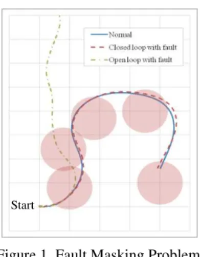
To illustrate the masking problem, a series of simulations were conducted using the aforementioned simulation model in 3D robot simulation software Gazebo. In each simulation five set points were given to the guidance program of the hovercraft. The set points are the centers of the red circles shown in Figure 1. Once the hovercraft enters a circle, it is guided to the next set point using the LOS guidance law. The simulations were done in three settings: normal, open loop, and closed loop. In the normal setting the hovercraft experienced no fault and followed the trajectory indicated with the solid line. During this simulation the thrusts that
the control program commanded to the two motors were recorded, and in the next simulation the recorded thrusts were applied to the hovercraft. This setting is referred to the open loop simulation in Figure 1. Therefore, with this setting there was no feedback in the control loop.
In this open loop simulation, a fault was assumed to occur on the left motor and that the left thrust was reduced by 20% due to the fault. In this case, as indicated with the dash-dot line, the hovercraft fails to follow the set points, and it becomes evident after the second set point that the hovercraft experiences an abnormality. On the contrary, when the feedback controller compensates the error in the trajectory due to the fault, as indicated with the dashed line, the hovercraft is able to follow the set points, and the fault is masked. This case study demonstrates the need of a fault detection and identification (FDI) technique that can reveal faults masked by feedback controllers.
Figure 1. Fault Masking Problem
2.1.The Control-Theoretic Framework to Differentiate Faults from Disturbances
The control-theoretic framework is informed by enlisting model-based fault detection and isolation methods proposed by various investigators over the past decades (Dinca, Aldemir, & Rizzoni, 1999; Isermann, 1984; Jones, 1973; Massoumnia, Verghese, & Willsky, 1989; Willsky, 1976). Among them, Kalman filtering and its variants, failure sensitive filters, multiple hypotheses filter-detection and isolation methods, jump process formulations and innovation based detection systems have been proposed and applied to a variety of engineering processes. The general structure of model-based methods builds upon analytical redundancy, definition of residuals, i.e. the differences between the sensory measurements and analytically obtained values. From our perspective, it is essential to consider the deviation of the residuals from white noise: the combined result of noise/disturbance and fault, assuming that the fault signature is a logical pattern showing which residuals are normal or which ones result from fault conditions.
Figure 2. Failure detection system involving a failure sensitive primary filter (here, denotes information concerning detected failures).
Figure 2 depicts a typical failure detection system involving a failure-sensitive filter. Failure sensitive filters track the system sensitivity to new data, reflect the presence of abrupt changes in the filter behavior and are applicable to a wide variety of faults/failures. Multiple hypotheses filter detection methods rely on a bank of linear filters based on different system hypotheses. They employ a wide range of adaptive estimation and failure detection strategies and aim at both system identification and state estimation.
In general, the system dynamics may be described by a nonlinear stochastic model of the form:
(1) where x(t) is the state of the system, u(t) is the control input, xc(t) is a measure of the fault dimension, specifically an internal motor resistance in these experiments; n(t) represents unmodeled dynamics and modeling errors; and (t) is the disturbance term. The difference xc(t) – (t) is a representation of the innovation or discrepancy between the fault value at time t and the disturbance. Dynamic response due to a fault, xc(t), is masked by the disturbance when the fault is below a specific threshold, and therefore the fault will not affect the modeled system dynamics.
The particle filtering formulation pursued in this paper avoids linearity and Gaussian noise assumptions typically found in most fault diagnosis and identification methods. The fault progression is often nonlinear and, consequently, the model should be nonlinear as well. Thus, the diagnostic model is described by
(2)
xd(t) represents two Boolean terms that correspond to normal (no-fault) and fault condition. It is employed to declare the fault condition when the innovation xc(t) – (t) reaches a specified threshold. The latter is determined by a stated confidence level and given false alarm rate. The particle filtering scheme for fault diagnosis allows for an easy and convenient determination of the confidence level in terms of overlapping areas between the fault and disturbance pdfs.
The available measurements are denoted by y(t):
(3)
where v(t) represents the measurement noise.
An alternative representation of the fault progression model that includes the impact of load or fatigue stresses on the progression of the fault dimension is expressed as:
(4)
where β is the time-varying parameter that describes the effect of stress conditions.
A particle-filter-based fault detection routine using the model allows for a statistical characterization of both Boolean and continuous-valued states, as new feature data (measurements) are received. As a result, at any given instant of time, this framework will provide an estimate of the probability masses associated with each fault mode, as well as a pdf estimate for meaningful physical variables in the system. Once this information is available within the fault detection module, it is conveniently processed to generate proper fault alarms and to inform about the statistical confidence of the detection routine. The outputs of the detection module may be defined as the expectations of the Boolean states in xd(t). This approach provides a recursively updated estimate of the probability for each fault condition considered in the analysis. These expectations may activate alarm indicators if they exceed appropriate thresholds for the probability of detection (typically 90% or 95%). This is a particularly useful approach when the normal operation of the system is defined through a dynamic state-space model. In addition, it is also possible to define the output of the detection module as the statistical confidence needed to declare the fault via hypothesis testing. This test is performed employing the pdf estimate of the continuous valued state in model (1) and another pdf defining the system disturbance. This approach allows for the inclusion of variables with a physical meaning into the decision-making procedure. Additionally, it is particularly useful when diagnosing deviations from a specified set-point, since historical data can be used to build the disturbance pdf.
2.2.Particle Filtering for Diagnosis – Distinguishing Faults from Disturbances
Figure 3. Schematic Diagram of the Closed-loop System In the closed-loop system, Figure 3, the direct path consists of the controller, the actuator and the plant (system), of which the latter two may contain a fault. For example, in the hovercraft model, the plant could be the motor driving the thruster fan or the motor-fan combination or even the total hovercraft model with its motion dynamics. Feedback control reduces the sensitivity of the system output to changes in the components of the direct path, disturbances affecting the system, and noise. As potential faults exist in this diagram as unmodeled dynamics within the actuators or mechanical system, they are unrecognizable from disturbances to the controller and may be masked by the control law.
2.3.The Solution Method
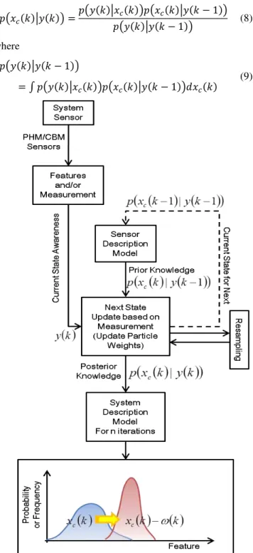
Figure 4 depicts a conceptual schematic of a particle filtering framework for fault diagnosis and, eventually, filtering of the innovation term, xc(t) – (t). Available and recommended sensors, specifically designed to monitor fault conditions, and the feature extraction module provide the sequential observation (or measurement) data of the fault growth process at time instant t = k.
(5)
where is the probability density function of
. The fault dimension at time t = k is written as:
(6)
with representing the corresponding pdf. It is from this fault progression model that the diagnostic model in (2) may be derived.
The first part of the approach is state estimation, i.e., estimating the current fault dimension and other important changing parameters of the environment. The a priori state estimation is generated from the knowledge of the previous state estimation and the process model according to
(7)
Incorporating the observation data into the a priori state estimate produces the posterior state estimation
(8)
where
(9)
The posterior result is a better estimate and adapts to changing data characteristics.
In general, no closed-form solution exists for estimating the state from the above equation except in the special case where the system dynamic model is linear, and the noise processes and are Gaussian. In this case, the Kalman filter is the optimal solution. For the diagnosis of complex systems, because of the nonlinear nature and ambiguity of the underlying dynamics of the physical systems, these functions are nonlinear and non-Gaussian, and hence, the Kalman filter cannot be used directly. Particle filtering approximates probability distributions using samples or “particles” having associated discrete probability masses. As the number of particles becomes very large this set of samples and weights tends to the true distribution, and the particle filter become the optimal Bayesian solution. Unfortunately, it is often not possible and too computationally expensive to sample directly from the posterior distribution. This problem is circumvented by assuming a known, easy to sample, importance distribution
. The real distributions would then be approximated by the importance distribution and the corresponding normalized importance weights for the ith sample
(10)
In the posterior state estimation, we need to update the importance weights. The update procedure is given by
(11)
A common choice is to select the prior distribution as
. This
procedure, referred to as Sequential Importance Sampling (SIS), often suffers from degeneracy problems. A selection step (resampling) may be introduced to eliminate particles with low importance ratios and reward those with high ratios. The resampling procedure maps the previously weighted random measure onto a new equally weighted random measure , by sampling again uniformly from the particle set
with respective probabilities . In the current study, the measurements are identical to the feature. The feature vector may be extracted from data (measurements) in general or a number of suitable features may be fused into a single one and represented by . Thus, the fault evolution is the same in this case as the feature The distribution pdf is computed from historical data or system measurements under normal
operating conditions. It may be time-varying or assumed to be stochastic without a time-varying profile. The procedure starts with the output measurements (or the feature values) whose pdf combines the fault mode and the disturbance. A schematic representation of the two (normalized) pdfs is shown in Figure 5.
Figure 5. A Concept of Innovation Between Faults and Disturbance
As a first approximation, we may consider a linear stochastic model (system dynamics) of the form:
(12) The particle filtering technique, as mentioned previously, addresses the nonlinear formulation and makes no assumptions beyond those dictated by the approximation of the actual pdf in terms of a discreet particle population. Thus, this approach exploits data and disturbance/noise profiles as they appear in the real system (hovercraft platform, in our case).
prescribed confidence and given false alarm rate from the disturbance.
3.THE AUTONOMOUS PLATFORM:HOVERCRAFT
We have designed and built a novel autonomous system-a hovercraft, shown in Figure 6. We are exploiting features of autonomy, flexibility, and data availability to demonstrate how fault modes are injected, monitored and distinguished from disturbances. The hovercraft is instrumented to monitor internal and external events continuously while appropriate software is used to detect fault conditions. Of particular interest are those concepts that will allow the detection of fault modes masked or hidden by feedback control loops. Care has been taken in the design of sensors, actuators, and navigation/control algorithms to enable the injection of critical faults and the demonstration of the “masking” effect. The enabling technologies will improve the vehicle’s autonomy attributes and permit the development, design, and implementation of novel autonomous systems.
The hovercraft hardware platform consists of a Pandaboard (Pandaboard, 2013), a low powered single-board computer, used for onboard computing. Robot Operating System (ROS) (Quigley et al., 2009) is used as middleware that connects various software modules such as localization, a position controller, and hardware drivers. For indoor localization HectorSLAM (Kohlbrecher, von Stryk, Meyer, & Klingauf, 2011) is employed. One advantage of using HectorSLAM is that localization and mapping can be done simultaneously without odometry information and with only LIDAR. For outdoor operations IMU and GPS can be added to improve localization results.
Figure 6. Hovercraft prototype.
Figure 7. Control system block diagram.
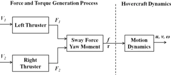
The position control is carried out by a line-of-sight (LOS) guidance law adapted from Breivik and Fossen (Breivik & Fossen, 2008) and a dynamic inversion controller. The LOS guidance law determines a desired surge speed and yaw angle, and the dynamic inversion controller generates the motor command that is required to meet the two desired properties. Nonlinear techniques such as the dynamic inversion heavily rely on accurate knowledge of plant dynamics and are often vulnerable to modeling errors (Brinker & Wise, 2012). To enhance robustness of the controller adaptation logic based on an artificial neural network is added to the controller. The adaptation logic handles various sources of uncertainties such as unmodeled dynamics and nonlinearities (Adams & Banda, 1993; Brinker & Wise, 2012; Buffington, Adams, & Banda, 1993). A block diagram of the hovercraft control loop is shown in Figure 7. The hovercraft is represented here by the mechanical system; the thruster motors 1 and 2 drive the fans that generate the forward thrust component; control signals V1 and V2 drive motors 1 and 2, respectively. The
controller decided upon monitors the current vehicle state (position, x, y; velocity, vx, vy; and heading, ) and, in the event of a discrepancy, generates command signals to correct for such deviations. The controller produces proper control signals that minimize the errors between the desired states from the reference model and the actual states of the hovercraft.
For communication between the hovercraft and a ground control center, the hovercraft is equipped with a wireless router. The body of the hovercraft is made of plywood, and the skirt is made of nylon. The nylon skirt is sealed with silicon for better air-tightness.
Figure 8. Gazebo simulation environment. 3.1.Hovercraft Configuration
The hovercraft is actuated by two independent uni-directional thrusters that are symmetrically located with respect to the plane of symmetry of the vehicle. This configuration is generating the hovercraft's surge force and yaw moment. Since there is no direct control input applied to the sway motion the hovercraft is classified as an under-actuated system. The input of each thruster is a voltage signal that controls an electrical motor. The motor speed is operating the thruster's propeller that generates the propulsion force. Four lift fans are used to provide the vehicle’s hover (upward) motion. The hovercraft model is divided into two parts. The first subsystem is related to the force and moment generation process. The second subsystem is associated with the hovercraft's motion dynamics. The two subsystems and their connections are shown in Figure 9.
Figure 9. Hovercraft dynamics model.
The first step towards the development of the hovercraft's equations of motion is the definition of two reference frames. Figure 10 shows an inertial frame, x and y, and a hovercraft body fixed from, xb and yb.
We consider only the planar 2-D motion of the vehicle disregarding the pitch, roll, and heave motion components. Denote by the hovercraft angular velocity and by the surge and sway velocities, respectively. From standard results, the hovercraft dynamic equations, with respect to the body fixed frame, are
(13)
where denotes the net surge force, the net yaw moment, is the mass of the hovercraft, is the inertia of the hovercraft (assuming symmetry with respect to the principal axis), and is additive noise due to disturbances.
Figure 10. Schematic of the hovercraft vehicle in Earth-fixed and body-Earth-fixed frames.
The two propulsion thrusts are produced by two identical fans that are operated by two identical motors. The last step of the modeling process is to include a simplified model of these motors. Denote by the voltage applied to the fan motor. This voltage is the output from the control system. From standard results, the electrical part of the motor is described by the following equation:
(14)
where is the motor current, is the motor resistance and is the back-emf voltage of the motor. The available measurements are all the states related to the motion of the vehicle , , the applied voltages to each motor and the produced currents . Since the produced current of each motor is considered a measured quantity, the current-voltage mapping is required by the fault detection and identification approach. Therefore,
(15)
where b is a constant, Kt is the motor torque constant, and KΩ is the back emf constant.
4.DIAGNOSIS OF MASKED FAULTS
4.1.Fault Model
The proposed analysis involves faults that are monotonically increasing functions of the load conditions. It is generally acknowledged that fault modes in engineered systems exhibit a monotonically increasing trend. The fault growth may pause or remain constant for short periods of time but the fault dimension (crack length, insulation breakdown, etc., as typical examples) will not exhibit a downward trend. A monotonic fault behavior ensures a surjective feature-to-fault mapping, or that the feature domain may be mapped onto the fault domain to produce an indirect measure of the fault. In this case study the load variable is the faulty motor current, . Therefore, the generic growth rate of the fault under consideration is given by the following differential equation:
(16)
with . By we denote the time instant that the fault initiates, while is the value of the faulty resistance. Furthermore, . The latter condition guarantees that the fault value is non-decreasing over time. Hence, the faulty resistance can be written as , where is the healthy value of the resistance and .
4.2.Feature Extraction
Feature or condition indicator selection and extraction constitutes the cornerstone for accurate and reliable fault diagnosis. A feature or condition indicator is an extracted value from a signal that describes the status of the process that fault diagnosis is applied to. Fault diagnosis depends mainly on extracting a set of features from sensor data that can distinguish between fault classes of interest, detect and isolate a particular fault at its early initiation stages (Zhang et al., 2011). Feature extraction may be approached in a number of ways, but in general, it is highly dependent on the application domain. In the hovercraft system, feature extraction is conducive to derivation from physics-of-failure mechanisms. The physical system is modeled with as much fidelity as needed to determine the effects of the fault on measurable quantities, for instance the effect of a change in motor thrust output on the velocity or orientation of the vehicle as compared to the expected system dynamics. Feature evaluation and selection metrics include the monotonicity of the relationship between the feature and the true fault size and the variance (or covariance) of the feature at discrete fault levels compared to the feature range (Voulgaris & Sconyers, 2010). A feature is sufficient if it shows a similar growth pattern to that of the ground truth data.
With the possibility of alternate fault types or multiple simultaneous faults, it is assumed that a feature or set of features may be estimated to identify only the fault of
interest. Alternatively, a single feature may accommodate a set of similar fault types, such as a set of faults that have similar characteristics at the component or system level. For this paper, only one fault is being examined.
As indicated previously, the fault under consideration is the change in the resistance value of one of the two motors. The hovercraft model is composed of two interconnected subsystems: the force/moment generation and the motion dynamics subsystems. The faulty resistance affects the force/moment generation directly, and subsequently the vehicle's motion. The goal of this paper is to use features extracted from signals generated by both subsystems. The first feature belongs to the force/moment generation subsystem and is the resistance value itself. In particular, we may write:
(17)
The second feature is derived from the motion dynamic subsystems. Both features are based on the dynamic equation of motion of the vehicle given in (13). The input-output description of each thruster is given by
(18)
where
(19)
Therefore from (13), the dynamics of the surge velocity can be written as
(20)
Assuming that we monitor the left motor for a fault and considering the above equation, the second feature is
(21)
The second feature is the mapping from the voltage-to-thrust. This feature is valid only when indicating the intuitive notion that the faulty motor must be operating in order to diagnose the fault. Similarly the dynamics of the angular motion are given by
(22)
The voltage-to-thrust mapping can be also derived by the angular motion as well. More specifically,
(23)
used by the detection algorithm. Typically, for the sensing of the vehicle's motion an Inertial Measurement Unit (IMU) is used. In such cases, it is preferable to monitor motion variables related to the angular motion of the vehicle since they typically have better accuracy compared to variables related to the linear motion and are less affected by disturbances and varying environmental conditions.
The angular response feature empirically estimates the deviation in expected angular velocity according to thrust effort supplied to the fan motors and the current measured angular velocity. The higher order angular response is less subjected to deviations in the environment, therefore the extraction of is as follows:
(24)
where is a root-mean-square operation over a sliding window of size samples, , are the left and right thrust efforts, is the heading of the hovercraft, and is a normalizing constant that is adapted during healthy operation. Because the feature is extracted using a window of samples, the feature has an accuracy and a lag proportional to the size of the window.
4.3.The Fault Detection and Identification Algorithm
A fault diagnosis procedure involves the tasks of fault detection and isolation, and fault identification (assessment of the severity of the fault). In general, this procedure may be interpreted as the fusion and utilization of the information present in a feature vector (measurements), with the objective of determining the operating condition (state) of a system and the causes for deviations from particularly desired behavioral patterns. Several ways to categorize FDI techniques can be found in literature. FDI techniques are classified according to the way that data is used to describe the behavior of the system: data-driven or model-based approaches.
Data-driven FDI techniques usually rely on signal processing and knowledge-based methodologies to extract the information hidden in the feature vector (also referred to as measurements). In this case, the classification/prediction procedure may be performed on the basis of variables that have little (or sometimes completely lack of) physical meaning. On the other hand, model-based techniques, as the name implies, use a description of a system (models based on first principles or physical laws) to determine the current operating condition.
A compromise between both classes of FDI techniques is often needed when dealing with complex nonlinear systems, given the difficulty of collecting useful faulty data (a critical aspect in any data-driven FDI approach) and the expertise needed to build a reliable model of the monitored system (a key issue in a model-based FDI approach).
From a nonlinear Bayesian state estimation standpoint, this compromise between data-driven and model-based techniques may be accomplished by the use of a particle filter (PF) based module built upon the dynamic state model describing the time progression or evolution of the fault (Orchard, 2007; Orchard & Vachtsevanos, 2007, 2009). The fault progression is often nonlinear and, consequently, the model should be nonlinear as well. Thus, the diagnostic model is described in (2).
Since the noise signal is a measure of uncertainty associated with Boolean states, it is advantageous to define its probability density through a random variable with bounded domain. For simplicity, may be assumed to be uniform white noise (Orchard, 2007). The PF approach using the above model allows statistical characterization of both Boolean and continuous-valued states, as new feature data (measurements) are received. As a result, at any given instant of time, this framework provides an estimate of the probability densities associated with each fault mode, as well as a probability distribution function (PDF) estimate for meaningful physical variables in the system. Hypothesis testing through calculating current and baseline PDFs is used to generate fault alarms, and other statistical analysis tools may be used to extract additional information about the detection and diagnostic results, discussed in the sequel. One particular advantage of the proposed particle filtering approach is the ability to characterize the evolution in time of the above mentioned nonlinear model through modification of the probability masses associated with each particle, as new data from fault indicators are received. The PF based FDI module is implemented accordingly using a non-linear time growth model given in (16) to describe the faulty motor's resistance value. A growth function is selected that as closely models the expected growth pattern as possible, in this case a C1 -discontinuous linear growth model. The rate of growth is estimated from a priori physics of failure models. The goal is for the algorithm to make an early detection of the increase to the resistance value (leading to an open-circuit). Two main operating conditions are distinguished: The normal condition reflects the fact that there is no fault in the motor while a faulty condition indicating an unexpected growth to the resistance value. Denote by and two Boolean states that indicate normal and faulty conditions respectively. Additional Boolean states may be added for larger fault spaces. The nonlinear model is given by
(25)
and
where
(27)
In the above equations is the initial healthy value of the resistance. The condition indicators and , after the addition of , are thresholded to restrict them to Boolean values, with the possibility of changing to new values at . The above system can be written in a more compact form as
(28)
(29)
where , , and
. The steps of the PF algorithm execution are described below:
1. From (28) generate state estimates (particles) denoted by where .
2. From (29) calculate the feature estimates, substituting the particles to the mapping .
3. Calculate the errors with
, and assign to each particle a weight , where denotes the standard normal distribution.
4. Normalize the weights . The normalized weights
represent the discrete probability masses of each state estimate.
5. Calculate the final state estimate using weighted sum of all the states .
Figure 11. Block diagram of the PF algorithm for fault estimation. (Raptis & Vachtsevanos, 2011)
An important part of the PF algorithm is the re-sampling procedure. Re-sampling is an action that takes place to counteract the degeneracy of the particles caused by estimates that have very low weights. A block diagram of the PF algorithm is given in Figure 11.
5.RESULTS
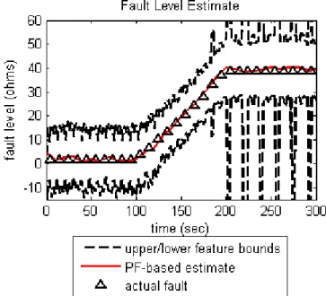
The performance of the proposed FDI algorithm was tested via numerical simulations and hardware tests. The hovercraft dynamics are described in (12) and the thrusters model in (13) and (14). The resistance fault is seeded to the left motor according to (15). The actual fault can be seen in Figure 12. The number of particles used for the estimator was .
Figure 12. Particle filter-based fault estimate and actual seeded fault value during simulation test.
The estimator fault value can be seen in Figure 12. Besides detecting the faulty condition, it is desired to obtain some measure of the statistical confidence of the alarm signal. For this reason, an additional output will be extracted from the FDI module. This output is the statistical confidence needed to declare the fault via hypothesis testing ( : The motor is healthy versus : The motor is faulty). The latter output needs another PDF to be considered as the baseline. The statistical parameters of the baseline PDF are derived from known healthy data, typically collected from the beginning of a component's lifecycle when it is known that no fault exists or any fault is negligible. In this case, a normal distribution is used to define this baseline data. The standard deviation represents the variation from the mean due to the random estimation error of the particle filter. This is a component of the total disturbance/noise term we are attempting to distinguish from the current fault. This indicator is essentially equivalent to an estimate of type II error, or equivalently the probability of detection.
The statistical confidence can be seen in Figure 13. Customer specifications for false alarm rate and fault detection confidence (constant red line) are respectively translated into acceptable margins for the type I and type II
Weight update
errors (varying blue line) in the detection routine. If additional information is required, it is possible to compute the value of the Fisher Discriminant Ratio (Duda, Hart, & Stork, 2000).
Figure 13. Estimator confidence metric derived from type II statistical hypothesis testing.
The baseline PDF of the faulty resistance and the estimated one at times t=107sec and t=200sec can be seen in Figure 14 and Figure 15, respectively.
Figure 14. Baseline (left) and estimated (right) PDFs of the faulty resistance at t=107 sec.
Figure 15. Baseline (left) and estimated (right) PDFs of the faulty resistance at t=200 sec.
Hardware tests were designed to observe the efficacy of the features on-board the physical hovercraft system. The motor winding fault was seeded as a reduced efficiency in the left motor response. This seeded fault was introduced as a percentage reduction in thrust effort expected from the navigation control output.
Four discrete fault levels were chosen and the hovercraft was commanded to follow the same designated set of
waypoints for three repetitions at each fault level: 0%, 30%, 50%, and 70% of thrust loss. Figure 16 shows the statistical behavior of angular response feature (blue bar lines) to each fault level during the hardware tests.
By using the same hardware test data and varying the RMS window size (number of samples) for filtering consecutive feature-based estimates, we observe the response of feature to variations in vehicle dynamics and environmental conditions. Using larger window sizes (Figure 16c), variations may be smoothed out, reducing the feature variance. The trade-off for increased feature accuracy is a larger lag time, as observed in the decrease of feature variance with the increase in window size . A statistical profile of the feature response may be empirically derived and used to guide the fault size estimation in the diagnostic, and eventually prognostic, particle filtering scheme. In general, this improved statistical profile may be used to enable early fault detection despite input feature lag times.
uncertainty. Improved feature accuracy, therefore, improves the diagnostic particle filter fault estimation accuracy.
6. CONCLUSIONS
Incipient failures or faults masked or hidden by feedback control loops tend to degrade performance of aerospace and other complex systems/processes and may even result in instability conditions. The early recognition and accurate differentiation of masked faults from typical plant disturbances compensated by such control loops may result in improved system performance and significant savings the operation of complex systems. The masking problem requires new and innovative tools and methods to verify the existence and impact of this event and the development and validation of detection, identification and control strategies aimed to remedy adverse situations arising from masking. We introduced in this contribution a control-theoretic framework for addressing the fault detection and differentiation between real faults and system disturbances. A laboratory autonomous hovercraft is used as the testbed for validation and demonstration purposes. Results are encouraging and may encourage further research into this important problem area. Such issues as multiple fault modes and actual experiments on prototypical platforms will enhance the present findings and allow relevant applications to large-scale aircraft and autonomous systems.
ACKNOWLEDGEMENT
We gratefully acknowledge the support and active contributions to this program of the NASA Ames Research Center. The work reported in this paper was funded under a subcontract from Impact Technologies—the prime NASA contracting company. We also acknowledge the collaboration between Impact personnel and Georgia Tech. REFERENCES
Adams, R. J., & Banda, S. S. (1993). An Integrated Approach to Flight Control Design Using Dynamic Inversion and Mu-Synthesis. Proceedings of the 1993 American Control Conference, Vols 1-3, 1385-1389.
Breivik, M., & Fossen, T. I. (2008). Guidance laws for planar motion control. Paper presented at the Decision and Control, 2008. CDC 2008. 47th IEEE Conference on.
Brinker, J. S., & Wise, K. A. (2012). Stability and flying qualities robustness of a dynamic inversion aircraft control law. Journal of Guidance Control and Dynamics, 19(6), 1270-1277. doi: Doi 10.2514/3.21782
Buffington, J. M., Adams, R. J., & Banda, S. S. (1993). Robust, nonlinear, high angle-of-attack control design for a supermaneuverable vehicle. Paper presented at the
AIAA Guidance, Navigation and Control Conference, Monterey, CA.
Dinca, L., Aldemir, T., & Rizzoni, G. (1999). A model-based probabilistic approach for fault detection and identification with application to the diagnosis of automotive engines. Automatic Control, IEEE Transactions on, 44(11), 2200-2205.
Duda, R. O., Hart, P. E., & Stork, D. H. (2000). Pattern Classification (2nd ed.), Wiley Interscience.
Ioannou, P. A., & Sun, J. (1996). Robust Adaptive Control. New Jersey, Prentice Hall.
Isermann, R. (1984). Process fault detection based on modeling and estimation methods—A survey. Automatica, 20(4), 387-404.
Jones, H. L. (1973). Failure detection in linear systems. Massachusetts Institute of Technology.
Khalil, H. K. (2002). Nonlinear Systems, 3rd. New Jewsey, Prentice Hall.
Koenig, N., & Howard, A. (2004). Design and use paradigms for gazebo, an open-source multi-robot simulator. Paper presented at the Intelligent Robots and Systems, 2004.(IROS 2004). Proceedings. 2004 IEEE/RSJ International Conference on.
Kohlbrecher, S., von Stryk, O., Meyer, J., & Klingauf, U. (2011). A flexible and scalable slam system with full 3d motion estimation. Paper presented at the Safety, Security, and Rescue Robotics (SSRR), 2011 IEEE International Symposium on.
Massoumnia, M. A., Verghese, G. C., & Willsky, A. S. (1989). Failure detection and identification. Automatic Control, IEEE Transactions on, 34(3), 316-321.
OpenDynamicsEngine. (2013). Open Dynamics Engine. from http://www.ode.org/
Orchard, M. E. . (2007). A Particle Filtering-based Framework for On-line Fault Diagnosis and Failure Prognosis. (Ph.D.), Georgia Institute of Technology, Atlanta, GA.
Orchard, M. E., & Vachtsevanos, G. J. (2007). A particle filtering-based framework for real-time fault diagnosis and failure prognosis in a turbine engine. Paper presented at the Control & Automation, 2007. MED'07. Mediterranean Conference on.
Orchard, M. E., & Vachtsevanos, G. J. (2009). A particle-filtering approach for on-line fault diagnosis and failure prognosis. Transactions of the Institute of Measurement and Control, 31(3-4), 221-246.
Quigley, M., Gerkey, B., Conley, K., Faust, J., Foote, T., Leibs, J., . . . Ng, A. (2009). ROS: an open-source Robot Operating System. Paper presented at the ICRA workshop on open source software.
Srivastava, A. N. (2012). Greener aviation with virtual sensors: a case study. Data Mining and Knowledge Discovery, 1-29.
Voulgaris, Z., & Sconyers, C. (2010). A Novel Feature Evaluation Methodology for Fault Diagnosis. Paper presented at the Proceedings of the World Congress on Engineering and Computer Science.
Willsky, A. S. (1976). A survey of design methods for failure detection in dynamic systems. Automatica, 12(6), 601-611.
Zhang, B., Sconyers, C., Byington, C., Patrick, R., Orchard, M. E., & Vachtsevanos, G. (2011). A probabilistic fault detection approach: application to bearing fault detection. Industrial Electronics, IEEE Transactions on, 58(5).
BIOGRAPHIES
Christopher Sconyers earned a double B.D. degree in Electrical Engineering and Computer Science from Texas A&M University in 2004 and a M.S. in Electrical and Computer Engineering from the Georgia Institute of Technology in 2006. He joined the Intelligent Control Systems Laboratory (ICSL) in 2007 and completed his Ph.D. research at the Georgia Institute of Technology in 2012. His areas of research include prognostics and health management (PHM), vision systems and unmanned aerial vehicles (UAVs). As part of his PHM research, he has designed and implemented tools for component level feature extraction, early fault detection and diagnosis, and failure prognosis for electrical, mechanical, hydraulic, and pneumatic subsystems In the area of UAVs and vision systems, he has developed methods for target tracking and geo-location from multiple mobile UAV platforms using limited sensor measurements and target data.
Young-Ki Lee is a Research Engineer II in Aerospace Systems Design Laboratory (ASDL) at School of Aerospace Engineering, Georgia Institute of Technology. He received his doctoral degree from Georgia Tech in 2008. His primary areas of research interest include unmanned vehicles, Robotics, Machine Learning, and Fault Diagnostics. Prior to joining Georgia Tech, he was a Gas Turbine Application Engineer at GE Energy.
Kilsoo Kim earned a Ph.D. degree in Aerospace Engineering from the Georgia Institute of Technology in 2011. He started a Postdoctoral Fellow at the ASDL in 2011. His research areas include robust, optimal, nonlinear, adaptive control, prognostics and health management (PHM), vibration, aeroelastics, finite element methods,
UAV, and Robotics. As part of his adaptive control research, he has designed and implemented Neural network (NN) based adaptive control for flight dynamics, an aeroelastic transport model, and synthetic jet flying wing. He made patents in the output feedback adaptive control area.
Sehwan Oh is a Ph.D. candidate in the ASDL at the Georgia Institute of Technology since 2010. His research areas include system design, design for autonomy and robotics.
Dimitri Mavris is the Boeing Professor of Advanced Aerospace Systems Analysis at the Guggenheim School of Aerospace Engineering, Georgia Institute of Technology, and the director of its Aerospace Systems Design Laboratory (ASDL). He received his B.S., M.S. and Ph.D. in Aerospace Engineering from the Georgia Institute of Technology. His primary areas of research interest include: advanced design methods, aircraft conceptual and preliminary design, air-breathing propulsion design, multi-disciplinary analysis, design and optimization, system of systems, and non-deterministic design theory Dr. Mavris has co-authored with his students in excess of 450 publications. He is currently Fellow of the American Institute of Aeronautics and Astronautics (AIAA) and a Fellow of the National Institute of Aerospace.. Dr. Mavris is also the recipient of the NSF CAREER award. Academically, Dr. Mavris has been awarded Georgia Tech’s prestigious Outstanding Development of Graduate Assistants Award in 1999 and 2004, and in 2000 he received the SAE's Ralph T. Teetor Educator of the Year Award. He is the director of the Center of Excellence in Robust Systems Design and Optimization under the General Electric University Strategic Alliance (GE USA).
Dr. Rodney Martin is a researcher at NASA Ames Research Center, Moffett Field, CA. His research interests include the intersection of control theory, machine learning and detection & estimation theory. He has worked in application areas ranging from data mining for aviation safety and space propulsion to computational sustainability for intelligent building control and operations. He has authored or co-authored over 20 conference or poster papers, journal articles, technical reports and a book chapter. Dr. Martin earned the B.S. degree in Mechanical Engineering from Carnegie-Mellon University in 1992, an M.S. degree in mechanical engineering from UC Berkeley in 2000, and a Ph.D. in Mechanical Engineering from UC Berkeley in 2004.