JHEP05(2011)064
Published for SISSA by SpringerReceived: February 22, 2011
Accepted: May 3, 2011
Published:May 12, 2011
Strange particle production in pp collisions at
√
s
=
0.9 and 7 TeV
CMS collaboration
E-mail: [email protected]
Abstract: The spectra of strange hadrons are measured in proton-proton collisions,
recorded by the CMS experiment at the CERN LHC, at centre-of-mass energies of 0.9 and 7 TeV. The K0
S, Λ, and Ξ− particles and their antiparticles are reconstructed from
their decay topologies and the production rates are measured as functions of rapidity and transverse momentum, pT. The results are compared to other experiments and to
pre-dictions of the Pythia Monte Carlo program. The pT distributions are found to differ
substantially from thePythia results and the production rates exceed the predictions by up to a factor of three.
Keywords: Hadron-Hadron Scattering
JHEP05(2011)064
Contents1 Introduction 1
2 CMS experiment and collected data 2
3 Strange particle reconstruction 3
4 Efficiency correction 5
5 Systematic uncertainties 8
6 Results 11
6.1 DistributionsdN/dy and dN/dpT 12
6.2 Analysis ofpT spectra 12
6.3 Analysis of production rate 16
7 Conclusions 20
1 Introduction
Measurements of particle yields and spectra are an essential step in understanding proton-proton collisions at the Large Hadron Collider (LHC). The Compact Muon Solenoid (CMS) Collaboration has published results on spectra of charged particles at centre-of-mass ener-gies of 0.9, 2.36, and 7 TeV [1,2]. In this analysis the measurement is extended to strange mesons and baryons (K0
S, Λ, Ξ−)
1 at centre-of-mass energies of 0.9 and 7 TeV. The
in-vestigation of strange hadron production is an important ingredient in understanding the nature of the strong force. The LHC experiments ALICE and LHCb have recently re-ported results on strange hadron production at√s= 0.9 TeV [3,4]. In addition to results at√s= 0.9 TeV, we also present results at √s= 7 TeV, opening up a new energy regime in which to study the strong interaction. As the strange quark is heavier than up and down quarks, production of strange hadrons is generally suppressed relative to hadrons contain-ing only up and down quarks. The amount of strangeness suppression is an important component in Monte Carlo (MC) models such asPythia [5] and hijing/bb[6]. Because the threshold for strange quark production in a quark-gluon plasma is much smaller than in a hadron gas, an enhancement in strange particle production has frequently been suggested as an indication of quark-gluon plasma formation [7]. This effect would be further enhanced in baryons with multiple strange quarks. While a quark-gluon plasma is more likely to be found in collisions of heavy nuclei, the enhancement of strange quark production in high
JHEP05(2011)064
energy pp collisions would be a sign of a collective effect, according to some models [8,9]. In contrast, recent Regge-theory calculations indicate little change in the ratio of K0
Sto charge
particle production with increasing collision energy [10,11]. Thus, these measurements can be used to constrain theories, provide input for tuning of Monte Carlo models, and serve as a reference for the interpretation of strangeness production results in heavy-ion collisions. Minimum bias collisions at the LHC can be classified as elastic scattering, inelastic single-diffractive dissociation (SD), inelastic double-diffractive dissociation, and inelastic non-diffractive scattering. The results presented here are normalized to the sum of double-diffractive and non-double-diffractive interactions, referred to as non-single-double-diffractive (NSD) in-teractions [1, 2]. This choice is made to most closely match the event selection and to compare with previous experiments, which often used similar criteria. The K0
S, Λ, and
Ξ− are long-lived particles (cτ > 1 cm) and can be identified from their decay products
originating from a displaced vertex. The particles are reconstructed from their decays: K0
S→π
+π−, Λ→pπ−, and Ξ−→Λπ− over the rapidity range|y|<2, where the rapidity
is defined asy= 12lnEE−p+pL
L,Eis the particle energy, andpLis the particle momentum along
the anticlockwise beam direction. For each particle species, we measure the production rate versus rapidity and transverse momentumpT, the average pT, the central production rate
dN
dy|y≈0, and the integrated yield for|y|<2 per NSD event. We compare our measurements
to results from Monte Carlo models and lower energy data.
2 CMS experiment and collected data
CMS is a general purpose experiment at the LHC [12]. The silicon tracker, lead-tungstate crystal electromagnetic calorimeter, and brass-scintillator hadron calorimeter are all im-mersed in a 3.8 T axial magnetic field while muon detectors are interspersed with flux return steel outside of the 6 m diameter superconducting solenoid. The silicon tracker is used to reconstruct charged particle trajectories with |η|<2.5, where the pseudorapidity is defined asη=−ln tanθ2,θbeing the polar angle with respect to the anticlockwise beam. The tracker consists of layers of 100×150µm2 pixel sensors at radii less than 15 cm and
layers of strip sensors, with pitch ranging from 80 to 183 µm, covering radii from 25 to 110 cm. In addition to barrel and endcap detectors, CMS has extensive forward calorimetry including a steel and quartz-fibre hadron calorimeter (HF), which covers 2.9< |η|<5.2. The data presented in this paper were collected by the CMS experiment in spring 2010 from proton-proton collisions at centre-of-mass energies of 0.9 and 7 TeV during a period in which the probability for two collisions in the same bunch crossing was negligible and the bunch crossings were well separated.
JHEP05(2011)064
determine the acceptance and efficiency, minimum-bias Monte Carlo samples were gener-ated at both centre-of-mass energies using Pythia 6.422 [5] with tune D6T [13]. These events were passed through a CMS detector simulation package based on Geant4 [14].
3 Strange particle reconstruction
Ionization deposits recorded by the silicon tracker are used to reconstruct tracks. To maximize reconstruction efficiency, we use a combined track collection formed from merging tracks found with the standard tracking described in ref. [15] and the minimum bias tracking described in ref. [1]. Both tracking collections use the same basic algorithm; the differences are in the requirements for seeding, propagating, and filtering tracks.
As described in ref. [15], the K0S and Λ (generically referred to as V 0
) reconstruction combines pairs of oppositely charged tracks; if the normalized χ2 of the fit to a common
vertex is less than 7, the candidate is kept. The primary vertex is refit for each candidate, re-moving the two tracks associated with the V0candidate. The next two paragraphs describe the selection of candidates for measurement of V0and Ξ−properties, respectively. Selection
variables are measured in units of σ, the calculated uncertainty including all correlations. To remove K0
Sparticles misidentified as Λ particles and vice versa, the K0S(Λ) candidates
must have a correspondingpπ−(π+π−) mass more than 2.5σ away from the world-average
Λ(K0
S) mass. The production cross sections we measure are intended to represent the
prompt production of K0
S and Λ, including strong and electromagnetic decays. However,
V0 particles can also be produced from weak decays and from secondary nuclear
inter-actions. These unwanted contributions are reduced by requiring that the V0 momentum vector points back to the primary vertex. This is done by requiring the 3D distance of closest approach of the V0 to the primary vertex to be less than 3σ. To remove generic
prompt backgrounds, the 3D V0vertex separation from the primary vertex must be greater than 5σ and both V0 daughter tracks must have a 3D distance of closest approach to the
primary vertex greater than 3σ. With the above selection, the background level for low transverse-momentum Λ candidates remains high. Therefore, additional cuts are applied to Λ candidates withpT <0.6 GeV/c:
• 3D separation between the primary and Λ vertices>10σ (instead of>5σ),
• transverse (2D) separation between the pp collision region (beamspot) and Λ vertex >10σ (instead of no cut), where the uncertainty is dominated by the Λ vertex, and
• 3D impact parameter of the pion and proton tracks with respect to the primary vertex > (7−2|y|)σ (instead of > 3σ) where y is the rapidity of the Λ candidate. The rapidity dependence is a consequence of the observation that, for the low trans-verse momentum candidates, large backgrounds dominate at small rapidity, while low efficiency characterizes the large rapidity behaviour.
The resulting mass distributions of K0
S and Λ candidates from the 0.9 and 7 TeV data are
shown in figures1 and2. Theπ+π− mass distribution is fit with a double Gaussian (with
JHEP05(2011)064
]
2
invariant mass [MeV/c −
π + π
450 500 550 600
2
Candidates / 1 MeV/c
0 20 40 60 80 100 3 10 × 3 10 × Yield: 1393 2 Mean: 497.8 MeV/c
2 : 8.4 MeV/c
σ
Avg
CMS
= 0.9 TeV s
]
2
invariant mass [MeV/c −
π + π
450 500 550 600
2
Candidates / 1 MeV/c
0 100 200 300 400 3 10 × 3 10 × Yield: 6534 2 Mean: 497.8 MeV/c
2 : 8.2 MeV/c
σ
Avg
CMS
= 7 TeV s
Figure 1. The π+π− invariant mass distributions from data collected at√s= 0.9 TeV (left) and 7 TeV (right). The solid curves are fits to a double Gaussian and quadratic polynomial. The dashed curves show the quadratic background contribution.
]
2
invariant mass [MeV/c −
π p
1100 1120 1140
2
Candidates / 0.5 MeV/c
0 5 10 15 20 3 10 × 3 10 × Yield: 276 2 Mean: 1116.1 MeV/c
2 : 3.6 MeV/c
σ
Avg
CMS
= 0.9 TeV s
]
2
invariant mass [MeV/c −
π p
1100 1120 1140
2
Candidates / 0.5 MeV/c
0 20 40 60 80 100 120 3 10 × 3 10 × Yield: 1460 2 Mean: 1116.0 MeV/c
2 : 3.4 MeV/c
σ
Avg
CMS
= 7 TeV s
Figure 2. The pπ−
invariant mass distributions from data collected at √s= 0.9 TeV (left) and 7 TeV (right). The solid curves are fits to a double Gaussian signal and a background function given byAqB, where q=M
pπ−−(mp+mπ−). The dashed curves show the background contribution.
is fit with a double Gaussian (common mean) signal function and a background function of the formAqB, whereq=Mpπ−−(mp+mπ−),Mpπ− is thepπ
− invariant mass, andA and
Bare free parameters. The fitted K0
S(Λ) yields at √
s= 0.9 and 7 TeV are 1.4×10⁶(2.8 ×10⁵)
and 6.5×10⁶(1.5
×106), respectively.
To reconstruct the Ξ−, charged tracks of the correct sign are combined with Λ
candi-dates. The χ2 probability of the fit to a common vertex for the Λ and the charged track
JHEP05(2011)064
]
2
invariant mass [MeV/c −
π Λ
1300 1350 1400
2
Candidates / 2 MeV/c
0 0.2 0.4 0.6 0.8 1 1.2 1.4 1.6 3 10 × 3 10 × Yield: 6.2 2 Mean: 1322.2 MeV/c
2 : 4.3 MeV/c
σ
Avg
CMS
= 0.9 TeV s
]
2
invariant mass [MeV/c −
π Λ
1300 1350 1400
2
Candidates / 2 MeV/c
0 2 4 6 8 3 10 × 3 10 × Yield: 34.4 2 Mean: 1322.1 MeV/c
2 : 4.1 MeV/c
σ
Avg
CMS
= 7 TeV s
Figure 3. The Λπ− invariant mass distributions from data collected at√s= 0.9 TeV (left) 7 TeV (right). The solid curves are fits to a double Gaussian signal and a background function given by Aq1/2+Bq3/2, where q = M
Λπ− −(mΛ +mπ−). The dashed curves show the background contribution.
world-average mass [16]. The primary vertex is refit for each Ξ− candidate, removing all
tracks associated with the Ξ−. The Ξ− candidates must then pass the following selection
criteria:
• 3D impact parameter with respect to the primary vertex >2σ for the proton track from the Λ decay,>3σ for theπ− track from the Λ decay, and>4σfor theπ−track from the Ξ− decay,
• invariant mass from the π+π− hypothesis for the tracks associated with the Λ
can-didate at least 20 MeV/c2 away from the world-average K0 S mass,
• 3D impact parameter of the Ξ− candidate with respect to the primary vertex<3σ,
• 3D separation between Λ vertex and primary vertex >10σ, and
• 3D separation between Ξ− vertex and primary vertex >2σ.
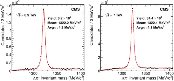
The mass distributions of Ξ− candidates from the √s= 0.9 and 7 TeV data are shown in
figure 3. The Λπ− mass is fit with a double Gaussian (with a common mean) signal
func-tion and a background funcfunc-tion of the formAq1/2+Bq3/2, where q=M
Λπ−−(mΛ+mπ−)
and MΛπ− is the Λπ
− invariant mass. The fitted Ξ− yields at √s = 0.9 and 7 TeV are
6.2×10³ and 3.4×10⁴, respectively.
4 Efficiency correction
JHEP05(2011)064
observed track multiplicity in data, as this has been shown to be an important component of the trigger efficiency [1, 2]. This is referred to as track weighting. The efficiency cor-rection also accounts for the other decay channels of the strange particles that we do not attempt to reconstruct, such as K0S→π
0
π0.
The efficiency is given by the number of reconstructed particles divided by the number of generated particles, subject to two modifications. Firstly, the efficiency correction is used to account for candidates from SD events. As the results are normalized to NSD events, candidates from SD events which pass the event selection must be removed. This is done by defining the efficiency as the number of reconstructed candidates in all events divided by the number of generated candidates in NSD events. Secondly, the efficiency is modified to account for the small contribution of reconstructed non-prompt strange particles which pass the selection criteria. This is only an issue for the Λ particles which receive contributions from Ξ and Ω decays. Since these non-prompt Λ particles are present in both the MC and data, we modify the efficiency to remove this contribution by calculating the numerator using all of the reconstructed strange particles and the denominator with only the prompt generated strange particles. As the MC fails to produce enough Ξ particles (see section6), the non-prompt Λ’s are weighted more than prompt Λ’s in the efficiency calculation.
The results of this analysis are presented in terms of two kinematic distributions: transverse momentum and rapidity. For all modes, |y| is divided into 10 equal size bins from 0 to 2 andpT is divided into 20 equal size bins from 0 to 4 GeV/c plus one bin each
from 4 to 5 GeV/c and 5 to 6 GeV/c. In addition, the V0 modes also have 6–8 GeV/c and 8–10 GeV/c pT bins. All results are for particles with|y|<2.
The efficiency correction for the V0 modes uses a two-dimensional binning in p T and |y|. Thus, the data are divided into 240 bins in the |y|, pT plane. The invariant mass
histograms in each bin are fit to a double Gaussian signal function (with a common mean) and a background function. In bins with few entries, a single Gaussian signal function is used. For the Λ sample, some bins are merged due to sparse populations in |y|, pT
space. The merging is performed separately when measuring |y| and pT such that the
merging occurs across pT and |y|bins, respectively. The efficiency from MC is evaluated
in each bin and applied to the measured yield to obtain the corrected yield. The two-dimensional binning used for the V0 efficiency correction greatly reduces problems arising
from remaining differences in production dynamics between the data and the simulation. The much smaller sample of Ξ− candidates prevents the use of 2D binning. Thus, the data
are divided into |y| bins to measure the|y|distribution and into pT bins to measure the
pT distribution. However, the MC spectra do not match the data. Therefore, each Monte
Carlo Ξ−particle is weighted inp
T(|y|) to match the distribution in data when measuring
the efficiency versus |y| (pT). Thus, the MC and data distributions are forced to match
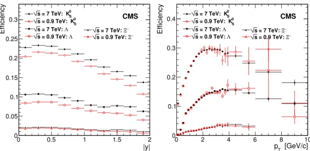
in the variable over which we integrate to determine the efficiency. We refer to this as kinematic weighting. The efficiencies for all three particles are shown versus |y|and pT in
figure4. The efficiencies (for particles with|y|<2) include the acceptance, event selection, reconstruction and selection, and also account for other decay channels. The increase in efficiency withpTis due to the improvement in tracking efficiency as trackpTincreases and
JHEP05(2011)064
|y|
0 0.5 1 1.5 2
Efficiency 0 0.05 0.1 0.15 0.2 0.25 0.3 0 S
= 7 TeV: K s
0 S
= 0.9 TeV: K s
Λ
= 7 TeV: s
Λ
= 0.9 TeV: s
−
Ξ
= 7 TeV: s
−
Ξ
= 0.9 TeV: s
CMS
[GeV/c]
T
p
0 2 4 6 8 10
Efficiency 0 0.1 0.2 0.3 0.4 0 S
= 7 TeV: K s
0 S
= 0.9 TeV: K s
Λ
= 7 TeV: s
Λ
= 0.9 TeV: s
−
Ξ
= 7 TeV: s
−
Ξ
= 0.9 TeV: s
CMS
Figure 4. Total efficiencies, including acceptance, trigger and event selection, reconstruction and particle selection, and other decay modes, as a function of|y| (left) andpT(right) for K0S, Λ, and
Ξ− produced promptly in the range
|y|<2. Error bars come from MC statistics.
due to particles decaying too far out to have reconstructed tracks. While there is no centre-of-mass energy dependence on the efficiency versus pT, particles produced at √s= 7 TeV
have a higher average-pT, resulting in a higher efficiency when plotted versus rapidity.
As a check on the ability of the Monte Carlo simulation to reproduce the efficiency, the (well-known) K0
S, Λ, and Ξ− lifetimes are measured. For the K0S measurement, the data
are divided into bins of pT and ct, wherect is calculated as ct=cmL/p wherem,L, and
pare, respectively, the mass, decay length, and momentum of the particle. In each bin the data is corrected by the MC efficiency and the corrected yields summed in pT to obtain
thectdistribution. Due to smaller sample sizes, the Λ and Ξ− yields are only measured in
bins ofct. Using the kinematic weighting technique, the MC efficiency in each bin ofct is calculated with thepT spectrum correctly weighted to match data. The corrected lifetime
distributions, shown in figure5, display exponential behaviour. The vertex separation re-quirements result in very low efficiencies and low yields in the first lifetime bin and are thus expected to have some discrepancies. An actual measurement of the lifetime would remove this issue by using the reduced proper time, where one measures the lifetime relative to the point at which the particle had a chance to be reconstructed. The measured values of the lifetimes are also reasonably consistent with the world averages [16] (shown in figure5) considering that only statistical uncertainties are reported and that this is not the optimal method for a lifetime measurement.
JHEP05(2011)064
ct [cm] 0 S K
0 2 4 6 8 10 12
-1
) dN / dct (cm)
NSD (1/N -2 10 -1 10 0.1 ps ± = 89.0 τ
= 7 TeV: s
0.2 ps
±
= 89.3
τ
= 0.9 TeV: s CMS 0.05 ps ± = 89.53 PDG τ Statistical uncertainties only
ct [cm]
Λ
0 2 4 6 8 10 12 14 16 18 20
-1
) dN / dct (cm)
NSD
(1/N
-2 10
-1
10 s = 7 TeV: τ = 261.4 ± 1.1 ps
3.1 ps
±
= 264.6
τ
= 0.9 TeV: s CMS 2.0 ps ± = 263.1 PDG τ Statistical uncertainties only
ct [cm]
−
Ξ
0 1 2 3 4 5 6 7 8 9 10
-1
) dN / dct (cm)
NSD (1/N -3 10 -2 10 5 ps ± = 167 τ
= 7 TeV: s
8 ps
±
= 178
τ
= 0.9 TeV: s CMS 1.5 ps ± = 163.9 PDG τ Statistical uncertainties only
Figure 5. K0
S (left), Λ (middle), and Ξ
− (right) corrected decay time distributions at√s= 0.9 and 7 TeV. The values of the lifetimes, derived from a fit with an exponential function (solid line), are shown in the legend along with the world-average value. The error bars and uncertainties on the lifetimes refer to the statistical uncertainty only.
weighted by the track multiplicity to reproduce the data). In the alternative method, the event selection efficiency versus track multiplicity is derived from the Monte Carlo. Then, each measured event is weighted by the inverse of the event selection efficiency based on its number of tracks. The number of events divided by the number of weighted events gives the event selection efficiency. However, since the event selection requires a primary vertex, no events will have fewer than two tracks. Therefore, the Monte Carlo is also used to determine the fraction of NSD events which have fewer than two tracks and the event selection efficiency is adjusted to include this effect. In both methods, the event selection efficiency accounts for unwanted SD events which pass the event selection. The numerator in the efficiency ratio contains all selected events, including single-diffractive events, while the denominator contains all NSD events.
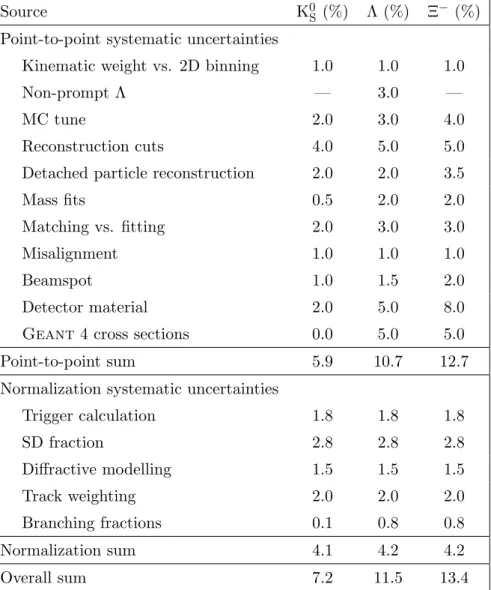
5 Systematic uncertainties
The systematic uncertainties, reported in table 1, are divided into two categories: nor-malization uncertainties, which only affect the overall nornor-malization, and point-to-point uncertainties, which may also affect the shape of the pT and |y|distributions.
The list below summarizes the source and evaluation of the point-to-point systematic uncertainties.
• Kinematic weighting versus 2D binning: The efficiency corrections using the 1D kine-matic weighting technique (used for the Ξ− analysis) and the 2D binning technique
(used for the V0 analysis) were compared by measuring the efficiency with both
methods on the highest statistics channel (K0
S at 7 TeV).
JHEP05(2011)064
• MC tune: The nominal efficiency calculated from the defaultPythia6 D6T tune [13] is compared to the efficiency obtained from thePythia6 Perugia0 (P0) tune [17] and Pythia8 [18].
• Variation of reconstruction cuts: The following cuts are varied for all three modes: V0 vertex separation significance (
±2σ), 3D impact parameter of V0 and Ξ− (±2σ),
3D impact parameter of tracks (±2σ), cut on K0
S(Λ) mass for Λ(K 0
S) candidates
(±1.5σ), and increase of number of hits required on each track from 3 to 5. For the Ξ−, additional cuts were varied: the Ξ−vertex separation significance (±1σ) and Ξ−
vertex fit probability (±3%).
• Detached particle reconstruction: Finding that the corrected lifetime distributions are exponential with the correct lifetime is a verification of our understanding of the reconstruction efficiency versus decay length. The systematic uncertainty is taken as the difference between the fitted lifetimes and the world-average lifetimes [16]. While the K0
S and Λ lifetimes are within 1% of the world-average, a 2% systematic
uncertainty is conservatively assigned.
• Mass fits: As an alternative to using a double-Gaussian signal shape, the V0 invariant
mass distributions are fit using a signal shape taken from Monte Carlo.
• Matching versus fitting: The number of reconstructed events, used in the numerator of the efficiency, is calculated in two ways. The truth matching method counts all reconstructed candidates which are matched to a generated candidate, based on the daughter momentum vectors and the decay vertex. The fitting method fits the MC mass distributions to extract a yield. The difference between these two is taken as a systematic.
• Misalignment: The nominal efficiency, obtained using a realistic alignment in the MC, is compared to the efficiency from a MC sample with perfect alignment.
• Beamspot: The location and width of the luminous region of pp collisions (beamspot) is varied in the simulation to assess the effect on efficiency.
• Detector material: The nominal efficiency is compared to the efficiency from a MC simulation in which the tracker was modified. The modification consisted of two parts. First, the mass of the tracker was increased by 5% which is a conservative estimate of the uncertainty. Second, the amounts of the various materials inside the tracker were adjusted within estimated uncertainties to obtain the tracker which maximized the interaction cross section. Both effects were implemented by changing material densities such that the tracker geometry remained the same. The effect is to decrease the efficiency as more particles, both primary and secondary, interact.
• Geant4 cross sections: The cross sections used by Geant4 for low energy strange
JHEP05(2011)064
As the trigger efficiency is used to derive the number of NSD events, it only affects the normalization. The normalization systematic uncertainties, most of which come from trigger efficiency uncertainties, are described below.
• Alternative trigger efficiency calculation: The difference between the default and al-ternative trigger efficiency measurements, described in section 4, is taken as the systematic uncertainty on the method.
• Fraction of SD vs NSD: The change in trigger efficiency when the fraction of single-diffractive events in Monte Carlo is varied by ±50% is taken as the systematic un-certainty on the fraction of SD events. The Pythia6 MC produces approximately 20% SD events while the fraction in the triggered data is considerably less [1, 2]. As the UA5 experiment measured 15.5% for this fraction at 900 GeV [20], a variation of ±50% is conservative.
• Modelling diffractive events: In addition to the fraction of SD events, the modelling of SD and NSD events may not be correct. The trigger efficiency obtained using the D6T tune is compared with the trigger efficiency from the P0 tune andPythia8. In par-ticular,Pythia8 uses a new Pomeron description of diffraction, modelled after PHO-JET [21,22], which results in a large increase in the track multiplicity of SD events.
• Track weighting: The track weighting of the Monte Carlo primarily affects the trigger efficiency. The track weighting requires a measurement of the track multiplicity distribution in data and MC. The default track multiplicity distribution is calculated from events which pass the trigger, except the primary vertex requirement is not applied. Two variations are considered. First, the track multiplicity distribution is measured from events also requiring a primary vertex. As this requires at least two tracks per event, the weight for events with fewer than two tracks is taken to be the same as the weight for events with two tracks. Second, the track weighting is determined with the primary vertex requirement (as in the first case), but without the HF trigger. The variation is taken as a systematic uncertainty on the track weighting.
• Branching fractions: The results are corrected for other decay channels of K0S, Λ,
and Ξ−. The branching fraction uncertainty reported by the PDG [16] is used as the
systematic uncertainty.
The systematic uncertainties at the two centre-of-mass energies are found to be essen-tially the same. The normalization uncertainties and the detached particle reconstruction uncertainty are obtained from the average of the results from the two centre-of-mass ener-gies. The other point-to-point systematic uncertainties are derived from the higher statis-tics 7 TeV results. The point-to-point systematic uncertainties are measured as functions of pT and |y| and found to be independent of both variables. Therefore, the systematic
JHEP05(2011)064
Source K0
S (%) Λ (%) Ξ− (%)
Point-to-point systematic uncertainties
Kinematic weight vs. 2D binning 1.0 1.0 1.0
Non-prompt Λ — 3.0 —
MC tune 2.0 3.0 4.0
Reconstruction cuts 4.0 5.0 5.0
Detached particle reconstruction 2.0 2.0 3.5
Mass fits 0.5 2.0 2.0
Matching vs. fitting 2.0 3.0 3.0
Misalignment 1.0 1.0 1.0
Beamspot 1.0 1.5 2.0
Detector material 2.0 5.0 8.0
Geant 4 cross sections 0.0 5.0 5.0
Point-to-point sum 5.9 10.7 12.7
Normalization systematic uncertainties
Trigger calculation 1.8 1.8 1.8
SD fraction 2.8 2.8 2.8
Diffractive modelling 1.5 1.5 1.5
Track weighting 2.0 2.0 2.0
Branching fractions 0.1 0.8 0.8
Normalization sum 4.1 4.2 4.2
Overall sum 7.2 11.5 13.4
Table 1. Systematic uncertainties for the K0
S, Λ, and Ξ
−
production measurements.
For the measurements of dN/dy, dN/dy|y≈0, and dN/dpT, the full systematic
uncer-tainty is applied. For the Λ/K0
S and Ξ−/Λ production ratio measurements, the largest
point-to-point systematic uncertainty of the two particles is used and, among the nor-malization systematic uncertainties, only the branching fraction correction is considered. Note that for the Ξ−/Λ production ratios, the Λ branching fraction uncertainty cancels in
the ratio.
6 Results
The results reported here are normalized to NSD interactions. The number of NSD raw events (given in section 2) are corrected for the trigger efficiency and the fraction of SD events after the selection. The corrected number of NSD events is 9.95×10⁶ and 37.10
×106
JHEP05(2011)064
6.1 Distributions dN/dy and dN/dpTThe corrected yields of K0
S, Λ, and Ξ−, versus|y|andpTare plotted in figure6, normalized
to the number of NSD events. The rapidity distribution is flat at central rapidities with a slight decrease at higher rapidities while the pT distribution is observed to be rapidly
falling. The rapidity distributions also show results from three different Pythia models:
Pythia 6.422 with the D6T and P0 tunes [13, 17] and Pythia 8.135 [18]. Fits to the
Tsallis function, described below, are overlaid on the pT distributions.
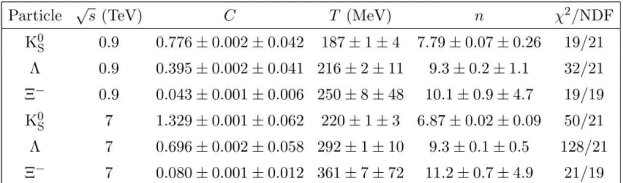
6.2 Analysis of pT spectra
The correctedpT spectra are fit to the Tsallis function [23], as was done for charged
parti-cles [1,2]. The Tsallis function used is:
1
NNSD
dN dpT
=C (n−1)(n−2)
nT[nT +m(n−2)]pT
1 +
q p2
T+m2−m
nT
−n
, (6.1)
whereCis a normalization parameter andT andnare the shape parameters. The results of the fits are shown in table2. The data points used in the fits include only the statistical un-certainty. The statistical uncertainties on the fit parameters are obtained from the fit. The systematic uncertainties are obtained by varying the cuts and Monte Carlo conditions (tune, material, beamspot, and alignment) in the same way as used to obtain the point-to-point systematic uncertainties on the distributions. The systematic uncertainty on the normaliza-tion parameterCalso includes the normalization uncertainty given in table1. The normal-izedχ2 indicates good fits to most of the samples. TheT parameter can be associated with
the inverse slope parameter of an exponential which dominates at low pT, while the n
pa-rameter controls the power law behaviour at highpT. While both parameters are necessary,
they are highly correlated, with correlation coefficients around 0.9, making it difficult to elu-cidate information. Nevertheless, it is clear thatT increases with particle mass and centre-of-mass energy. This indicates a broader low-pTshape at higher centre-of-mass energy and
for higher mass particles. In contrast, the high pT power-law behaviour seems to show a
much steeper fall off for the two baryons than for the K0
S. While the power-law behaviour
of the baryons does not show any dependence on the centre-of-mass energy, the fall off of the K0
S particles produced at
√s= 0.9 TeV is steeper than those produced at√s= 7 TeV.
We calculate the average pT directly from the data in the dN/dpT histograms. The
Tsallis function fit is used to obtain the correct bin centre and to account for events beyond the measured pT range, both of which are small effects. The statistical uncertainty on the
average pT is obtained by finding the standard deviation ofpT and dividing by the square
JHEP05(2011)064
|y|
S 0
K
0 0.5 1 1.5 2
) dN / dy
NSD (1/N 0 0.05 0.1 0.15 0.2 0.25 0.3 0.35
= 7 TeV s
PYTHIA6 D6T PYTHIA6 P0 PYTHIA8
= 0.9 TeV s PYTHIA6 D6T PYTHIA6 P0 PYTHIA8 CMS [GeV/c] T p 0 S K
0 2 4 6 8 10
-1
(GeV/c) T
) dN / dp
NSD (1/N -5 10 -4 10 -3 10 -2 10 -1 10 1
= 7 TeV s
= 0.9 TeV s
CMS
|y|
Λ
0 0.5 1 1.5 2
) dN / dy
NSD (1/N 0 0.05 0.1 0.15 0.2
= 7 TeV s
PYTHIA6 D6T PYTHIA6 P0 PYTHIA8
= 0.9 TeV s PYTHIA6 D6T PYTHIA6 P0 PYTHIA8 CMS [GeV/c] T p Λ
0 2 4 6 8 10
-1
(GeV/c) T
) dN / dp
NSD (1/N -6 10 -5 10 -4 10 -3 10 -2 10 -1 10
= 7 TeV s
= 0.9 TeV s CMS |y| − Ξ
0 0.5 1 1.5 2
) dN / dy
NSD (1/N 0 0.005 0.01 0.015 0.02
= 7 TeV s
PYTHIA6 D6T PYTHIA6 P0 PYTHIA8
= 0.9 TeV s PYTHIA6 D6T PYTHIA6 P0 PYTHIA8 CMS [GeV/c] T p − Ξ
0 1 2 3 4 5 6
-1
(GeV/c) T
) dN / dp
NSD (1/N -5 10 -4 10 -3 10 -2 10
= 7 TeV s
= 0.9 TeV s
CMS
Figure 6. K0
S(top), Λ (middle), and Ξ
−
(bottom) production per NSD event versus|y|(left) andpT
JHEP05(2011)064
Particle √s(TeV) C T (MeV) n χ2/NDF
K0
S 0.9 0.776±0.002±0.042 187±1±4 7.79±0.07±0.26 19/21
Λ 0.9 0.395±0.002±0.041 216±2±11 9.3±0.2±1.1 32/21 Ξ− 0.9 0.043±0.001±0.006 250±8±48 10.1±0.9±4.7 19/19
K0
S 7 1.329±0.001±0.062 220±1±3 6.87±0.02±0.09 50/21
Λ 7 0.696±0.002±0.058 292±1±10 9.3±0.1±0.5 128/21
Ξ− 7 0.080±0.001±0.012 361±7±72 11.2±0.7±4.9 21/19
Table 2. Results of fitting the Tsallis function to the data. In the C, T, and n columns, the first uncertainty is statistical and the second is systematic. The parameter values andχ2/NDF are
obtained from fits to the data with only the statistical uncertainty included.
√
s= 0.9 TeV √s= 7 TeV
Particle Data MC (D6T) Data MC (D6T)
K0
S 654±1±8 580 790±1±9 757
Λ 837±6±40 750 1037±5±63 1071
Ξ− 971±14±43 831 1236±11±72 1243
Table 3. AveragepT in units of MeV/c obtained from the appropriate dN/dpT distribution as
described in the text. Results fromPythia6 with tune D6T are also given. In each data column, the first uncertainty is statistical and the second is systematic.
averagepTfrom data andPythia6 with the D6T underlying event tune is shown in table3.
The Pythiavalues are quite close to the √s= 7 TeV data and somewhat lower than the
√
s= 0.9 TeV data. Although the averagepT results fromPythia are relatively close to
the data, thePythiapT distributions are significantly broader than the data distributions.
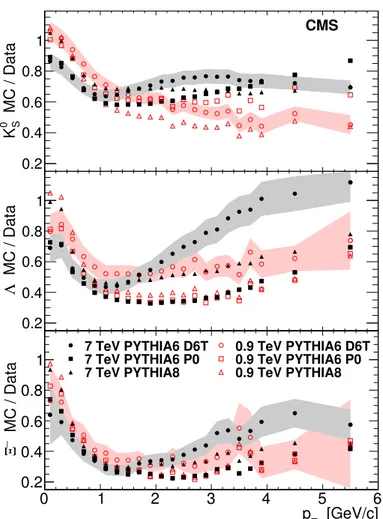
This disagreement can be seen in figure7, which shows the ratio ofPythiato data for pro-duction of K0S, Λ, and Ξ− versus transverse momentum. As well as a broader distribution,
thePythiadistributions also show significant variation as a function of tune and version. The relative production versus transverse momentum between different species is shown in figure 8. The N(Λ)/N(K0
S) and N(Ξ−)/N(Λ) distributions both increase with pT at
low pT, as expected from the higher averagepT for the higher mass particles. At higher
pT the N(Λ)/N(K0S) distribution drops off while the N(Ξ−)/N(Λ) distribution appears
to plateau. This is consistent with the values of the power-law parameter n for these distributions. Interestingly, the collision energy has no observable effect on the level or shape of these production ratios. The Pythiaresults are superimposed on the same plot. While Pythia reproduces the general features, it differs significantly in the details and shows large variations depending on tune and version.
Figure9shows a comparison of the CMSpTdistributions with results from other recent
JHEP05(2011)064
[GeV/c]
T
p
0 1 2 3 4 5 6
MC / Data
−
Ξ
0.2 0.4 0.6 0.8
1 7 TeV PYTHIA6 D6T7 TeV PYTHIA6 P0
7 TeV PYTHIA8
0.9 TeV PYTHIA6 D6T 0.9 TeV PYTHIA6 P0 0.9 TeV PYTHIA8
0 1 2 3 4 5 6
MC / Data
Λ
0.2 0.4 0.6 0.8 1
MC / Data
0 S
K
0.2 0.4 0.6 0.8 1
CMS
Figure 7. Ratio of MC production to data production of K0
S (top), Λ (middle), and Ξ
− (bottom) versus pT at √s = 0.9 TeV (open symbols) and √s= 7 TeV (filled symbols). Results are shown
for three Pythia predictions at each centre-of-mass energy. To reduce clutter, the uncertainty, shown as a band, is included for only one of the predictions (D6T) at each energy. This uncertainty includes the statistical and point-to-point systematic uncertainties added in quadrature but does not include the normalization systematic uncertainty.
distributions are multiplied by 8πpT, 4, and 8π, respectively. The CDF cross sections are
also divided by 49 mb (the NSD cross section used by CDF [25]) to obtain distributions nor-malized to NSD events, matching the CMS and STAR normalization. The ALICE results are normalized to inelastic events (including single diffractive events). The ALICE and CMS results at 0.9 TeV agree for all three particles. The distributions behave as expected, with higher centre-of-mass energy corresponding to increased production rates and harder spectra. To remove the effect of normalization, figure 10 shows a comparison of Λ to K0 S
and Ξ−to Λ production ratios versus transverse momentum. The CMS results agree with
the results from pp collisions at√s=0.2 TeV from STAR [24] and at√s=0.9 TeV results from ALICE [3]. These three results show a remarkable consistency across a wide variety of collision energies. In contrast, the CDF values for N(Λ)/N(K0
JHEP05(2011)064
[GeV/c]
T
p
0 2 4 6 8 10
)
0 S
) / N(K
Λ
N(
0 0.2 0.4 0.6 0.8 1
= 7 TeV s
PYTHIA6 D6T PYTHIA6 P0 PYTHIA8
= 0.9 TeV s
PYTHIA6 D6T PYTHIA6 P0 PYTHIA8
CMS
[GeV/c]
T
p
0 1 2 3 4 5 6
)
Λ
) / N(
−
Ξ
N(
0 0.05 0.1 0.15 0.2 0.25
= 7 TeV s
PYTHIA6 D6T PYTHIA6 P0 PYTHIA8
= 0.9 TeV s
PYTHIA6 D6T PYTHIA6 P0 PYTHIA8
CMS
Figure 8. N(Λ)/N(K0
S) (left) and N(Ξ
−
)/N(Λ) (right) in NSD events versus pT. The inner
vertical error bars (when visible) show the statistical uncertainties, the outer the statistical and all systematic uncertainties summed in quadrature. Results are shown for three Pythiapredictions at each centre-of-mass energy.
higher than the CMS results while the CDF measurements ofN(Ξ−)/N(Λ) [25] are lower,
albeit with less significance.
Reducing thepT distributions to a single value, the average pT, we compare the CMS
results with earlier results at lower energies in figure 11[3, 24, 26–32]. The CMS results are in excellent agreement with the recent ALICE measurements at 0.9 TeV. The CMS results continue the overall trend of increasing average pT with increasing particle mass
and increasing centre-of-mass energy.
6.3 Analysis of production rate
As a measure of the overall production rate in NSD events, dNdy|y≈0 and the total yield
for |y| <2 were extracted and tabulated in table 4. The quantity dNdy|y≈0 is the average
value of dNdy over the region |y| < 0.2. The integrated yields for |y|< 2 are obtained by integrating thepT spectra, using the Tsallis function fit to account for particles above the
measured pT range.
The central production rates of K0
S, Λ, and Ξ− are compared to previous results in
figure12. The results show the expected increase in production with centre-of-mass energy with little evidence of a difference due to beam particles. As the ALICE results are normal-ized to all inelastic collisions, they are expected to be somewhat lower than the CMS results.
The production ratiosN(K0
S)/N(Λ) andN(Ξ−)/N(Λ) versus|y|are shown in figure13.
The rapidity distributions are very flat and, as observed in thepT distributions of figure8,
JHEP05(2011)064
[GeV/c]
T
p
0 1 2 3 4 5 6
-1
(GeV/c)
T
/dp−
Ξ
) dN
NSD
(1/N 10-5
-4
10
-3
10
-2
10
CMS: pp @ 7 TeV CMS: pp @ 0.9 TeV
@ 1.96 TeV p
CDF: p
ALICE: pp @ 0.9 TeV STAR: pp @ 0.2 TeV
0 1 2 3 4 5 6
-1
(GeV/c)
T
/dp
Λ
) dN
NSD
(1/N
-4
10
-3
10
-2
10
-1
10
0 1 2 3 4 5 6
-1
(GeV/c)
T
/dp0 S
K
) dN
NSD
(1/N 10-4
-3
10
-2
10
-1
10
1
CMS
Figure 9. K0
S(top), Λ (middle), and Ξ
− (bottom) production per event versusp
T. The error bars
on the CMS results show the combined statistical, point-to-point systematic, and normalization systematic uncertainties. The error bars on the CDF [25], ALICE [3], and STAR [24] results show the combined statistical and systematic uncertainties. The CMS, CDF, and STAR results are normalized to NSD events while the ALICE results are normalized to all inelastic events.
seen in the comparisons shown in the left panes of figure 6; Pythia underestimates the production of strange particles and the discrepancy grows with particle mass.
Table5shows a comparison of the production rate of data to Pythia6 with the D6T tune. The left column shows a large increase in the strange particle production cross sec-tion as the centre-of-mass energy increases from 0.9 to 7 TeV. The systematic uncertainties for this ratio are reduced as the same uncertainty affects both samples nearly equally. The results for K0
S and Λ are consistent with the increase observed in inclusive charged particle
production [1,2] (5.82
3.48 = 1.67) while the Ξ
in-JHEP05(2011)064
[GeV/c]
T
p
0 1 2 3 4 5 6
)
Λ
) / N(
−
Ξ
N(
0 0.1 0.2 0.3
@ 1.96 TeV p
CDF: p
@ 1.8 TeV p
CDF: p
@ 0.63 TeV p
CDF: p
ALICE: pp @ 0.9 TeV STAR: pp @ 0.2 TeV
CMS: pp @ 7 TeV CMS: pp @ 0.9 TeV
0 1 2 3 4 5 6
)
0 S
) / N(K
Λ
N(
0.5 1 1.5
CMS
Figure 10. Ratio of Λ to K0
S production (top) and Ξ
− to Λ production (bottom) versusp
T. The
CMS, ALICE [3], and STAR [24] error bars include the statistical and systematic uncertainties. The CDF error bars include the statistical uncertainties for N(Λ)/N(K0
S) [26] and the statistical
and systematic uncertainties for N(Ξ−
)/N(Λ) [25]. The CDF N(Λ)/N(K0
S) bin sizes are doubled
to reduced fluctuations. For experiments in which the binning for Λ and Ξ− is different (ALICE and STAR), bins are merged to provide common bin ranges in theN(Ξ−
)/N(Λ) distribution.
√
s= 0.9 TeV √s= 7 TeV Particle dNdy|y≈0 N dNdy|y≈0 N
K0
S 0.205±0.001±0.015 0.784±0.002±0.056 0.346±0.001±0.025 1.341±0.001±0.097
Λ 0.108±0.001±0.012 0.404±0.004±0.046 0.189±0.001±0.022 0.717±0.005±0.082 Ξ− 0.011
±0.001±0.001 0.043±0.001±0.006 0.021±0.001±0.003 0.080±0.001±0.011
Table 4. dNdy|y≈0 and integrated yields (|y|<2.0) per NSD event from data. In each data column,
the first uncertainty is statistical and the second is systematic.
crease in particle production from 0.9 to 7 TeV is not well modelled byPythia6. Another feature, seen in the right column, is the deficit of strange particles produced by Pythia 6. The deficit of K0S particles in the MC, 15% (28%) low at 0.9 (7) TeV, is consistent with
the results found in the production of charged particles [1,2]. However, the deficit is much worse as the mass increases, resulting in a 63% reduction in Ξ− particles in MC compared
JHEP05(2011)064
[TeV]
s
-1
10 1 10
[GeV/c] − Ξ 〉 T p 〈 0.6 0.8 1
1.2 Ξ− CMS (pp) ) p E735 (p ALICE (pp) ) p UA5 (p STAR (pp) [GeV/c]Λ 〉 T p
〈 0.60.7
0.8 0.9 1 1.1 Λ CMS (pp) ) p CDF (p ) p E735 (p ALICE (pp) ) p UA5 (p STAR (pp) [GeV/c]0 S
K 〉 T p 〈 0.5 0.6 0.7 0.8 0 S K CMS (pp) ) p CDF (p ALICE (pp) ) p UA5 (p STAR (pp)
CMS
Figure 11. Average pT for K0S (top), Λ (middle), and Ξ
− (bottom), as a function of the centre-of-mass energy. The CMS measurements are for |y| < 2. The other results are from UA5 [27–31] (p¯p collisions covering|y|<2.5,|y|<2, and|y|<3 for K0
S, Λ, and Ξ
−
, respectively), E735 [32] (p¯p collisions using tracks with −0.36 < η < 1.0), CDF [26] (p¯p collisions covering |η| < 1.0), STAR [24] (pp collisions covering |y| < 0.5), and ALICE [3] (pp collisions covering |y|<0.75 for K0
S and Λ and|y|<0.8 for Ξ
−
). Some points have been slightly offset from the true energy to improve visibility. The vertical bars indicate the statistical and systematic uncertainties (when available) summed in quadrature.
Particle
" dN
dy|y≈0(7 TeV)
dN
dy|y≈0(0.9 TeV)
# "dN
dy|y≈0(MCD6T)
dN
dy|y≈0(Data)
#
Data MC (D6T) √s= 0.9 TeV √s= 7 TeV K0
S 1.69±0.01±0.06 1.42 0.852±0.005±0.061 0.717±0.001±0.052
Λ 1.75±0.02±0.08 1.48 0.606±0.007±0.070 0.514±0.003±0.059 Ξ− 1.93
±0.10±0.09 1.51 0.477±0.021±0.064 0.373±0.010±0.050
JHEP05(2011)064
[TeV]
s
-1
10 1 10
0
≈
y
/dy−
Ξ
) dN
ev
(1/N
0 0.005 0.01 0.015
0.02 0.025
− Ξ
CMS NSD (pp) ALICE INEL (pp) STAR NSD (pp)
0
≈
y
/dy Λ
) dN
ev
(1/N
0.1 0.15
0.2 Λ
CMS NSD (pp) ALICE INEL (pp) STAR NSD (pp)
0
≈
y
/dy0 S
K
) dN
ev
(1/N 0.1
0.15 0.2 0.25 0.3
0.35 S 0 K
CMS NSD (pp) ) p CDF MB (p ALICE INEL (pp)
) p UA5 NSD (p STAR NSD (pp)
CMS
Figure 12. The central rapidity production rate for K0
S (top), Λ (middle), and Ξ
− (bottom), as a function of the centre-of-mass energy. The previous results are from UA5 [29, 30] (p¯p), CDF [33] (p¯p), STAR [24] (pp), and ALICE [3] (pp). The CMS, UA5, and STAR results are normalized to NSD events. The CDF results are normalized to events passing their trigger and event selection defined chiefly by activity in both sides of the detector, at least four tracks, and a primary vertex. The ALICE results are normalized to all inelastic events. Some points have been slightly offset from the true energy to improve visibility. The vertical bars indicate the statistical uncertainties for the UA5 and CDF results and the combined statistical and systematic uncertainties for the CMS, ALICE, and STAR results.
7 Conclusions
This article presents a study of the production of K0S, Λ, and Ξ− particles in proton-proton
collisions at centre-of-mass energies 0.9 and 7 TeV. By fully exploiting the low-momentum track reconstruction capabilities of CMS, we have measured the transverse-momentum dis-tribution of these strange particles down to zero. From this sample of 10 million strange particles, the transverse momentum distributions were measured out to 10 GeV/c for K0 S
and Λ and out to 6 GeV/c for Ξ−. We fit these distributions with a Tsallis function to
ob-tain information on the exponential decay at lowpT and the power-law behaviour at high
pT. All species show a flattening of the exponential decay as the centre-of-mass energy
JHEP05(2011)064
|y|
0 0.5 1 1.5 2
)
0 S
) / N(K
Λ
N(
0 0.1 0.2 0.3 0.4 0.5 0.6 0.7
= 7 TeV s
PYTHIA6 D6T PYTHIA6 P0 PYTHIA8
= 0.9 TeV s
PYTHIA6 D6T PYTHIA6 P0 PYTHIA8
CMS
|y|
0 0.5 1 1.5 2
)
Λ
) / N(
−
Ξ
N(
0 0.02 0.04 0.06 0.08 0.1 0.12 0.14
= 7 TeV s
PYTHIA6 D6T PYTHIA6 P0 PYTHIA8
= 0.9 TeV s
PYTHIA6 D6T PYTHIA6 P0 PYTHIA8
CMS
Figure 13. The production ratios N(Λ)/N(K0
S) (left) and N(Ξ
−)/N(Λ) (right) in NSD events versus|y|. The inner vertical error bars (when visible) show the statistical uncertainties, the outer the statistical and all systematic uncertainties summed in quadrature. Results are shown for three Pythiapredictions at each centre-of-mass energy.
parameter decreases from 7.8 to 6.9. The average pT values, calculated directly from the
data, are found to increase with particle mass and centre-of-mass energy, in agreement with predictions and other experimental results. While the PythiapT distributions used
in this analysis show significant variation based on tune and version, they are all broader than the data distributions.
We have also measured the production versus rapidity and extracted the value ofdN/dy in the central rapidity region. The increase in production of strange particles as the centre-of-mass energy increases from 0.9 to 7 TeV is approximately consistent with the results for inclusive charged particles. However, as in the inclusive charged particle case,Pythiafails to match this increase. For K0
S production, the discrepancy is similar to what has been
found in charged particles. However, the deficit betweenPythia and data is significantly larger for the two hyperons at both energies, reaching a factor of three discrepancy for Ξ− production at√s= 7 TeV. If a quark-gluon plasma or other collective effects were present, we might expect an enhancement of double-strange baryons to single-strange baryons and/or an enhancement of strange baryons to strange mesons. However, the production ratios N(Λ)/N(K0
S) andN(Ξ−)/N(Λ) versus rapidity and transverse momentum show no
JHEP05(2011)064
AcknowledgmentsWe wish to congratulate our colleagues in the CERN accelerator departments for the excel-lent performance of the LHC machine. We thank the technical and administrative staff at CERN and other CMS institutes, and acknowledge support from: FMSR (Austria); FNRS and FWO (Belgium); CNPq, CAPES, FAPERJ, and FAPESP (Brazil); MES (Bulgaria); CERN; CAS, MoST, and NSFC (China); COLCIENCIAS (Colombia); MSES (Croatia); RPF (Cyprus); Academy of Sciences and NICPB (Estonia); Academy of Finland, ME, and HIP (Finland); CEA and CNRS/IN2P3 (France); BMBF, DFG, and HGF (Germany); GSRT (Greece); OTKA and NKTH (Hungary); DAE and DST (India); IPM (Iran); SFI (Ireland); INFN (Italy); NRF and WCU (Korea); LAS (Lithuania); CINVESTAV, CONA-CYT, SEP, and UASLP-FAI (Mexico); PAEC (Pakistan); SCSR (Poland); FCT (Portu-gal); JINR (Armenia, Belarus, Georgia, Ukraine, Uzbekistan); MST and MAE (Russia); MSTD (Serbia); MICINN and CPAN (Spain); Swiss Funding Agencies (Switzerland); NSC (Taipei); TUBITAK and TAEK (Turkey); STFC (United Kingdom); DOE and NSF (USA). Individuals have received support from the Marie-Curie programme and the European Re-search Council (European Union); the Leventis Foundation; the A. P. Sloan Foundation; the Alexander von Humboldt Foundation; the Associazione per lo Sviluppo Scientifico e Tecnologico del Piemonte (Italy); the Belgian Federal Science Policy Office; the Fonds pour la Formation `a la Recherche dans l’´ındustrie et dans l’ ´Agriculture (FRIA-Belgium); and the Agentschap voor Innovatie door Wetenschap en Technologie (IWT-Belgium).
The CMS collaboration author list
Yerevan Physics Institute, Yerevan, Armenia
V. Khachatryan, A.M. Sirunyan, A. Tumasyan
Institut f¨ur Hochenergiephysik der OeAW, Wien, Austria
W. Adam, T. Bergauer, M. Dragicevic, J. Er¨o, C. Fabjan, M. Friedl, R. Fr¨uhwirth, V.M. Ghete, J. Hammer1, S. H¨ansel, C. Hartl, M. Hoch, N. H¨ormann, J. Hrubec,
M. Jeitler, G. Kasieczka, W. Kiesenhofer, M. Krammer, D. Liko, I. Mikulec, M. Pernicka, H. Rohringer, R. Sch¨ofbeck, J. Strauss, A. Taurok, F. Teischinger, P. Wagner, W. Wal-tenberger, G. Walzel, E. Widl, C.-E. Wulz
National Centre for Particle and High Energy Physics, Minsk, Belarus
V. Mossolov, N. Shumeiko, J. Suarez Gonzalez
Universiteit Antwerpen, Antwerpen, Belgium
L. Benucci, K. Cerny, E.A. De Wolf, X. Janssen, T. Maes, L. Mucibello, S. Ochesanu, B. Roland, R. Rougny, M. Selvaggi, H. Van Haevermaet, P. Van Mechelen, N. Van Remortel
Vrije Universiteit Brussel, Brussel, Belgium
JHEP05(2011)064
Universit´e Libre de Bruxelles, Bruxelles, BelgiumO. Charaf, B. Clerbaux, G. De Lentdecker, V. Dero, A.P.R. Gay, G.H. Hammad, T. Hreus, P.E. Marage, L. Thomas, C. Vander Velde, P. Vanlaer, J. Wickens
Ghent University, Ghent, Belgium
V. Adler, S. Costantini, M. Grunewald, B. Klein, A. Marinov, J. Mccartin, D. Ryckbosch, F. Thyssen, M. Tytgat, L. Vanelderen, P. Verwilligen, S. Walsh, N. Zaganidis
Universit´e Catholique de Louvain, Louvain-la-Neuve, Belgium
S. Basegmez, G. Bruno, J. Caudron, L. Ceard, J. De Favereau De Jeneret, C. Delaere, P. Demin, D. Favart, A. Giammanco, G. Gr´egoire, J. Hollar, V. Lemaitre, J. Liao, O. Mil-itaru, S. Ovyn, D. Pagano, A. Pin, K. Piotrzkowski, N. Schul
Universit´e de Mons, Mons, Belgium
N. Beliy, T. Caebergs, E. Daubie
Centro Brasileiro de Pesquisas Fisicas, Rio de Janeiro, Brazil
G.A. Alves, D. De Jesus Damiao, M.E. Pol, M.H.G. Souza
Universidade do Estado do Rio de Janeiro, Rio de Janeiro, Brazil
W. Carvalho, E.M. Da Costa, C. De Oliveira Martins, S. Fonseca De Souza, L. Mundim, H. Nogima, V. Oguri, W.L. Prado Da Silva, A. Santoro, S.M. Silva Do Amaral, A. Sznajder, F. Torres Da Silva De Araujo
Instituto de Fisica Teorica, Universidade Estadual Paulista, Sao Paulo, Brazil
F.A. Dias, M.A.F. Dias, T.R. Fernandez Perez Tomei, E. M. Gregores2, F. Marinho,
S.F. Novaes, Sandra S. Padula
Institute for Nuclear Research and Nuclear Energy, Sofia, Bulgaria
N. Darmenov1, L. Dimitrov, V. Genchev1, P. Iaydjiev1, S. Piperov, M. Rodozov,
S. Stoykova, G. Sultanov, V. Tcholakov, R. Trayanov, I. Vankov
University of Sofia, Sofia, Bulgaria
M. Dyulendarova, R. Hadjiiska, V. Kozhuharov, L. Litov, E. Marinova, M. Mateev, B. Pavlov, P. Petkov
Institute of High Energy Physics, Beijing, China
J.G. Bian, G.M. Chen, H.S. Chen, C.H. Jiang, D. Liang, S. Liang, J. Wang, J. Wang, X. Wang, Z. Wang, M. Xu, M. Yang, J. Zang, Z. Zhang
State Key Lab. of Nucl. Phys. and Tech., Peking University, Beijing, China
Y. Ban, S. Guo, Y. Guo, W. Li, Y. Mao, S.J. Qian, H. Teng, L. Zhang, B. Zhu, W. Zou
Universidad de Los Andes, Bogota, Colombia
A. Cabrera, B. Gomez Moreno, A.A. Ocampo Rios, A.F. Osorio Oliveros, J.C. Sanabria
Technical University of Split, Split, Croatia
N. Godinovic, D. Lelas, K. Lelas, R. Plestina3, D. Polic, I. Puljak University of Split, Split, Croatia
Z. Antunovic, M. Dzelalija
Institute Rudjer Boskovic, Zagreb, Croatia
V. Brigljevic, S. Duric, K. Kadija, S. Morovic
University of Cyprus, Nicosia, Cyprus
JHEP05(2011)064
Charles University, Prague, Czech RepublicM. Finger, M. Finger Jr.
Academy of Scientific Research and Technology of the Arab Republic of Egypt, Egyptian Network of High Energy Physics, Cairo, Egypt
Y. Assran4, M.A. Mahmoud5
National Institute of Chemical Physics and Biophysics, Tallinn, Estonia
A. Hektor, M. Kadastik, K. Kannike, M. M¨untel, M. Raidal, L. Rebane
Department of Physics, University of Helsinki, Helsinki, Finland
V. Azzolini, P. Eerola
Helsinki Institute of Physics, Helsinki, Finland
S. Czellar, J. H¨ark¨onen, A. Heikkinen, V. Karim¨aki, R. Kinnunen, J. Klem, M.J. Ko-rtelainen, T. Lamp´en, K. Lassila-Perini, S. Lehti, T. Lind´en, P. Luukka, T. M¨aenp¨a¨a, E. Tuominen, J. Tuominiemi, E. Tuovinen, D. Ungaro, L. Wendland
Lappeenranta University of Technology, Lappeenranta, Finland
K. Banzuzi, A. Korpela, T. Tuuva
Laboratoire d’Annecy-le-Vieux de Physique des Particules, IN2P3-CNRS, Annecy-le-Vieux, France
D. Sillou
DSM/IRFU, CEA/Saclay, Gif-sur-Yvette, France
M. Besancon, S. Choudhury, M. Dejardin, D. Denegri, B. Fabbro, J.L. Faure, F. Ferri, S. Ganjour, F.X. Gentit, A. Givernaud, P. Gras, G. Hamel de Monchenault, P. Jarry, E. Locci, J. Malcles, M. Marionneau, L. Millischer, J. Rander, A. Rosowsky, I. Shreyber, M. Titov, P. Verrecchia
Laboratoire Leprince-Ringuet, Ecole Polytechnique, IN2P3-CNRS, Palaiseau, France
S. Baffioni, F. Beaudette, L. Bianchini, M. Bluj6, C. Broutin, P. Busson, C. Charlot,
T. Dahms, L. Dobrzynski, R. Granier de Cassagnac, M. Haguenauer, P. Min´e, C. Mironov, C. Ochando, P. Paganini, D. Sabes, R. Salerno, Y. Sirois, C. Thiebaux, B. Wyslouch7,
A. Zabi
Institut Pluridisciplinaire Hubert Curien, Universit´e de Strasbourg, Univer-sit´e de Haute Alsace Mulhouse, CNRS/IN2P3, Strasbourg, France
J.-L. Agram8, J. Andrea, A. Besson, D. Bloch, D. Bodin, J.-M. Brom, M. Cardaci, E.C. Chabert, C. Collard, E. Conte8, F. Drouhin8, C. Ferro, J.-C. Fontaine8, D. Gel´e,
U. Goerlach, S. Greder, P. Juillot, M. Karim8, A.-C. Le Bihan, Y. Mikami, P. Van Hove Centre de Calcul de l’Institut National de Physique Nucleaire et de Physique des Particules (IN2P3), Villeurbanne, France
F. Fassi, D. Mercier
Universit´e de Lyon, Universit´e Claude Bernard Lyon 1, CNRS-IN2P3, Institut de Physique Nucl´eaire de Lyon, Villeurbanne, France
JHEP05(2011)064
E. Andronikashvili Institute of Physics, Academy of Science, Tbilisi, GeorgiaL. Megrelidze, V. Roinishvili
Institute of High Energy Physics and Informatization, Tbilisi State University, Tbilisi, Georgia
D. Lomidze
RWTH Aachen University, I. Physikalisches Institut, Aachen, Germany
G. Anagnostou, M. Edelhoff, L. Feld, N. Heracleous, O. Hindrichs, R. Jussen, K. Klein, J. Merz, N. Mohr, A. Ostapchuk, A. Perieanu, F. Raupach, J. Sammet, S. Schael, D. Sprenger, H. Weber, M. Weber, B. Wittmer
RWTH Aachen University, III. Physikalisches Institut A, Aachen, Germany
M. Ata, W. Bender, M. Erdmann, J. Frangenheim, T. Hebbeker, A. Hinzmann, K. Hoepfner, C. Hof, T. Klimkovich, D. Klingebiel, P. Kreuzer, D. Lanske†, C. Magass,
G. Masetti, M. Merschmeyer, A. Meyer, P. Papacz, H. Pieta, H. Reithler, S.A. Schmitz, L. Sonnenschein, J. Steggemann, D. Teyssier
RWTH Aachen University, III. Physikalisches Institut B, Aachen, Germany
M. Bontenackels, M. Davids, M. Duda, G. Fl¨ugge, H. Geenen, M. Giffels, W. Haj Ah-mad, D. Heydhausen, T. Kress, Y. Kuessel, A. Linn, A. Nowack, L. Perchalla, O. Pooth, J. Rennefeld, P. Sauerland, A. Stahl, M. Thomas, D. Tornier, M.H. Zoeller
Deutsches Elektronen-Synchrotron, Hamburg, Germany
M. Aldaya Martin, W. Behrenhoff, U. Behrens, M. Bergholz9, K. Borras, A. Cakir,
A. Campbell, E. Castro, D. Dammann, G. Eckerlin, D. Eckstein, A. Flossdorf, G. Flucke, A. Geiser, I. Glushkov, J. Hauk, H. Jung, M. Kasemann, I. Katkov, P. Katsas, C. Kleinwort, H. Kluge, A. Knutsson, D. Kr¨ucker, E. Kuznetsova, W. Lange, W. Lohmann9, R. Mankel,
M. Marienfeld, I.-A. Melzer-Pellmann, A.B. Meyer, J. Mnich, A. Mussgiller, J. Olzem, A. Parenti, A. Raspereza, A. Raval, R. Schmidt9, T. Schoerner-Sadenius, N. Sen, M. Stein,
J. Tomaszewska, D. Volyanskyy, R. Walsh, C. Wissing
University of Hamburg, Hamburg, Germany
C. Autermann, S. Bobrovskyi, J. Draeger, H. Enderle, U. Gebbert, K. Kaschube, G. Kaussen, R. Klanner, J. Lange, B. Mura, S. Naumann-Emme, F. Nowak, N. Pietsch, C. Sander, H. Schettler, P. Schleper, M. Schr¨oder, T. Schum, J. Schwandt, A.K. Srivastava, H. Stadie, G. Steinbr¨uck, J. Thomsen, R. Wolf
Institut f¨ur Experimentelle Kernphysik, Karlsruhe, Germany
C. Barth, J. Bauer, V. Buege, T. Chwalek, W. De Boer, A. Dierlamm, G. Dirkes, M. Feindt, J. Gruschke, C. Hackstein, F. Hartmann, S.M. Heindl, M. Heinrich, H. Held, K.H. Hoff-mann, S. Honc, T. Kuhr, D. Martschei, S. Mueller, Th. M¨uller, M. Niegel, O. Oberst, A. Oehler, J. Ott, T. Peiffer, D. Piparo, G. Quast, K. Rabbertz, F. Ratnikov, M. Renz, C. Saout, A. Scheurer, P. Schieferdecker, F.-P. Schilling, G. Schott, H.J. Simonis, F.M. Sto-ber, D. Troendle, J. Wagner-Kuhr, M. Zeise, V. Zhukov10, E.B. Ziebarth
Institute of Nuclear Physics ”Demokritos”, Aghia Paraskevi, Greece
G. Daskalakis, T. Geralis, S. Kesisoglou, A. Kyriakis, D. Loukas, I. Manolakos, A. Markou, C. Markou, C. Mavrommatis, E. Ntomari, E. Petrakou
University of Athens, Athens, Greece
JHEP05(2011)064
University of Io´annina, Io´annina, GreeceI. Evangelou, C. Foudas, P. Kokkas, N. Manthos, I. Papadopoulos, V. Patras, F.A. Triantis
KFKI Research Institute for Particle and Nuclear Physics, Budapest, Hungary
A. Aranyi, G. Bencze, L. Boldizsar, G. Debreczeni, C. Hajdu1, D. Horvath11, A. Kapusi,
K. Krajczar12, A. Laszlo, F. Sikler, G. Vesztergombi12
Institute of Nuclear Research ATOMKI, Debrecen, Hungary
N. Beni, J. Molnar, J. Palinkas, Z. Szillasi, V. Veszpremi
University of Debrecen, Debrecen, Hungary
P. Raics, Z.L. Trocsanyi, B. Ujvari
Panjab University, Chandigarh, India
S. Bansal, S.B. Beri, V. Bhatnagar, N. Dhingra, R. Gupta, M. Jindal, M. Kaur, J.M. Kohli, M.Z. Mehta, N. Nishu, L.K. Saini, A. Sharma, A.P. Singh, J.B. Singh, S.P. Singh
University of Delhi, Delhi, India
S. Ahuja, S. Bhattacharya, B.C. Choudhary, P. Gupta, S. Jain, S. Jain, A. Kumar, R.K. Shivpuri
Bhabha Atomic Research Centre, Mumbai, India
R.K. Choudhury, D. Dutta, S. Kailas, S.K. Kataria, A.K. Mohanty1, L.M. Pant, P. Shukla Tata Institute of Fundamental Research - EHEP, Mumbai, India
T. Aziz, M. Guchait13, A. Gurtu, M. Maity14, D. Majumder, G. Majumder, K. Mazumdar,
G.B. Mohanty, A. Saha, K. Sudhakar, N. Wickramage
Tata Institute of Fundamental Research - HECR, Mumbai, India
S. Banerjee, S. Dugad, N.K. Mondal
Institute for Research and Fundamental Sciences (IPM), Tehran, Iran
H. Arfaei, H. Bakhshiansohi, S.M. Etesami, A. Fahim, M. Hashemi, A. Jafari, M. Khakzad, A. Mohammadi, M. Mohammadi Najafabadi, S. Paktinat Mehdiabadi, B. Safarzadeh, M. Zeinali
INFN Sezione di Bari a, Universit`a di Bari b, Politecnico di Bari c, Bari, Italy
M. Abbresciaa,b, L. Barbonea,b, C. Calabriaa,b, A. Colaleoa, D. Creanzaa,c, N. De
Filippisa,c, M. De Palmaa,b, A. Dimitrova, L. Fiorea, G. Iasellia,c, L. Lusitoa,b,1, G. Maggia,c, M. Maggia, N. Mannaa,b, B. Marangellia,b, S. Mya,c, S. Nuzzoa,b, N. Pacificoa,b, G.A. Pierroa, A. Pompilia,b, G. Pugliesea,c, F. Romanoa,c, G. Rosellia,b,
G. Selvaggia,b, L. Silvestrisa, R. Trentaduea, S. Tupputia,b, G. Zitoa
INFN Sezione di Bologna a, Universit`a di Bologna b, Bologna, Italy
G. Abbiendia, A.C. Benvenutia, D. Bonacorsia, S. Braibant-Giacomellia,b, L. Brigliadoria,
P. Capiluppia,b, A. Castroa,b, F.R. Cavalloa, M. Cuffiania,b, G.M. Dallavallea, F. Fabbria,
A. Fanfania,b, D. Fasanellaa, P. Giacomellia, M. Giuntaa, C. Grandia, S. Marcellinia, M. Meneghellia,b, A. Montanaria, F.L. Navarriaa,b, F. Odoricia, A. Perrottaa,
F. Primaveraa, A.M. Rossia,b, T. Rovellia,b, G. Sirolia,b, R. Travaglinia,b
INFN Sezione di Catania a, Universit`a di Catania b, Catania, Italy
S. Albergoa,b, G. Cappelloa,b, M. Chiorbolia,b,1, S. Costaa,b, A. Tricomia,b, C. Tuvea INFN Sezione di Firenze a, Universit`a di Firenze b, Firenze, Italy