Efficiency of genome-wide association study in open-pollinated populations

GABRIEL BORGES MUNDIM

EFFICIENCY OF GENOME-WIDE ASSOCIATION STUDY IN OPEN-POLLINATED POPULATIONS

Tese apresentada à Universidade Federal de Viçosa, como parte das exigências do Programa de Pós-Graduação em Genética e Melhoramento, para obtenção do título de Doctor Scientiae.

VIÇOSA

Ficha catalográfica preparada pela Biblioteca Central da Universidade Federal de Viçosa - Câmpus Viçosa

T

Mundim, Gabriel Borges, 1987-M965e

2016

Efficiency of genome-wide association study in

open-pollinated populations / Gabriel Borges Mundim. – Viçosa, MG, 2016.

ix, 48f. : il. ; 29 cm.

Orientador: José Marcelo Soriano Viana.

Tese (doutorado) - Universidade Federal de Viçosa. Referências bibliográficas: f.26-35.

1. Genética vegetal. 2. Genética quantitativa. 3. Milho -Melhoramento genético. I. Universidade Federal de Viçosa. Departamento de Biologia Geral. Programa de Pós-graduação em Genética e Melhoramento. II. Título.

ii

iii

AGRADECIMENTOS

Agradeço a Deus, pela sabedoria e por guiar os meus passos.

Aos meus pais, Edilson e Maria Perpétua, pelo amor, carinho, apoio e confiança em mim depositados.

À minha irmã Luísa, pela amizade e pelo carinho.

Aos meus avós, Oldemar (in memorian) e Purcínia, Jovino e Felinda, pelo carinho e orações.

À minha amada esposa Vanessa, pelo amor, companheirismo, paciência e por me apoiar em todos os momentos. Aos seus pais, José Francisco e Olga, pela amizade e confiança.

Aos meus demais familiares, pelo apoio, incentivo e amizade.

À Universidade Federal de Viçosa (UFV) e ao Programa de Pós-Graduação em Genética e Melhoramento, pela oportunidade.

Ao Conselho Nacional de Desenvolvimento Científico e Tecnológico (CNPq), à Coordenação de Aperfeiçoamento de Pessoal de Nível Superior (CAPES) e à Fundação de Amparo à Pesquisa do estado de Minas Gerais (FAPEMIG), pelo apoio financeiro.

Ao meu orientador, professor José Marcelo Soriano Viana, por sua orientação segura, amizade, incentivo, dedicação e pelos seus ensinamentos.

Aos professores Fabyano Fonseca e Silva, Vinícius Ribeiro Faria, ao Dr. Marcos Deon Vilela de Resende e ao Dr. Antônio Carlos Baião de Oliveira pela disponibilidade de participação na banca e pelas valiosas contribuições.

Aos colegas do Programa Milho-Pipoca, pelo trabalho em equipe, pela amizade e colaboração.

Aos amigos da Dow Agrosciences Sementes & Biotecnologia, pela oportunidade de trabalho e crescimento profissional.

A todos os meus amigos com os quais eu convivi desde a graduação, e a todos os companheiros de república, pela amizade, confiança e apoio.

A todos que contribuíram para o desenvolvimento desse trabalho e para a minha formação profissional.

iv BIOGRAFIA

GABRIEL BORGES MUNDIM, filho de Edilson Borges da Silva e Maria Perpétua Mundim Borges, nasceu em 15 de novembro de 1987, em Patos de Minas, Minas Gerais. Estudou na Escola Estadual "Coronel Cristiano", em Lagoa Formosa, Minas Gerais e concluiu o Ensino Médio em 2005, no Colégio Marista de Patos de Minas, Minas Gerais.

Em maio de 2006, ingressou no curso de Agronomia da Universidade Federal de Viçosa, obtendo o título de Engenheiro Agrônomo em janeiro de 2011.

Em março de 2011, iniciou o curso de Mestrado em Genética e Melhoramento pela Universidade Federal de Viçosa, obtendo o título de Magister Science em fevereiro de 2013.

v SUMÁRIO

LISTA DE TABELAS vi

LISTA DE FIGURAS vii

RESUMO viii

ABSTRACT Ix

1. Introduction 1

2. Materials and Methods 4

2.1. Quantitative genetics theory for GWAS in open-pollinated populations 4 2.2. Quantitative genetics theory for GWAS with inbred lines panel 8

2.3. Simulation 11

2.4. Statistical analyses 13

3. Results 16

4. Discussion 20

4.1. GWAS in open-pollinated populations: theoretical aspects, potential and limitations

20

4.2. GWAS in open-pollinated populations: influence of QTL heritability and sample size

21

4.3. GWAS in open-pollinated populations, inbred lines panel and RILs 24

5. Conclusion 27

6. Acknowledgments 28

vi

LISTA DE TABELAS

Table 1 Average number of significant associations with a FDR of 1 and 5%, power of QTL detection (%), number of false-positive associations in chromosomes with no QTL and one to four QTL, bias in the QTL position (cM), and average range for the regions with identified QTL, regarding population 1, generation 10r (random cross), three traits (expansion volume (EV; mL/g), grain yield (GY; g/plant), and days to maturity (DM)), two sample sizes, and two

heritabilities ………... 36

Table 2 Average number of significant associations with a FDR of 1 and 5%, power of QTL detection (%), number of false-positive associations in chromosomes with no QTL and one to two QTL, bias in the QTL position (cM), and average range for the regions with identified QTL, regarding population 1, generation 10r (random cross), three traits (expansion volume (EV; mL/g), grain yield (GY; g/plant), and days to maturity (DM)), two sample sizes, and QTL heritability of 12% ………... 37 Table 3 Average number of significant associations with a FDR of 1 and 5%, power of QTL detection (%), number of false-positive associations in chromosomes with no QTL and one to four QTL, bias in the QTL position (cM), and average range for the regions with identified QTL, regarding an inbred lines panel, three traits (expansion volume (EV; mL/g), grain yield (GY; g/plant), and days to maturity (DM)), two sample sizes, and two heritabilities ………. 38 Table 4 Average number of significant associations with a FDR of 1 and 5%, power of QTL detection (%), number of false-positive associations in chromosomes with no QTL and one to four QTL, bias in the QTL position (cM), and average range for the regions with identified QTL, regarding population 1, generation 10r10s (random cross and selfing), three traits (expansion volume (EV; mL/g), grain yield (GY; g/plant), and days to maturity (DM)), two sample sizes,

vii

LISTA DE FIGURAS

viii RESUMO

MUNDIM, Gabriel Borges, D. Sc., Universidade Federal de Viçosa, fevereiro de 2016. Eficiência do estudo de associação genômica ampla em populações de polinização aberta. Orientador: José Marcelo Soriano Viana. Coorientadores: Fabyano Fonseca e Silva e Rodrigo Oliveira de Lima.

ix ABSTRACT

MUNDIM, Gabriel Borges, D. Sc., Universidade Federal de Viçosa, February, 2016. Efficiency of genome-wide association study in open-pollinated populations. Adviser: José Marcelo Soriano Viana. Co-advisers: Fabyano Fonseca e Silva and Rodrigo Oliveira de Lima.

1 1. Introduction

Association analysis, also known as linkage disequilibrium (LD) mapping or association mapping, is a relatively new population-based approach used to identify marker-trait associations based on LD. Linkage disequilibrium, also known as gametic phase disequilibrium, gametic disequilibrium or allelic association, can be simply stated as the “non-random association of alleles at different loci” or the correlation between polymorphisms that is caused by their shared history of mutation and recombination (Flint-Garcia et al., 2003). Association analysis have been successful in detecting genes associated with diseases in humans (Kerem et al., 1989; Hastbacka et al., 1992; Sladek et al., 2007; Weiss et al., 2009), animals (Barendse et al., 2007; Kijas et al., 2009; Bolormaa et al., 2011; Fan et al., 2011) and different quantitative traits in plants (Thornsberry et al., 2001; Tian et al., 2011; Schaefer & Bernardo, 2013; Suwarno et al., 2015). There are two main association mapping strategies: the candidate gene approach, which focuses on polymorphisms in specific genes controlling traits of interest, and the genome-wide association studies (GWAS), which survey the entire genome for polymorphisms associated with complex traits (Risch & Merkangas, 1996).

2

resolution (Stuber et al., 1999; Flint-Garcia et al., 2005). Other advantages of GWAS are the reduction in cost and time to develop a mapping population (Yu & Buckler, 2006) and the possibility of evaluating a large number of alleles in diverse populations (Krill et al., 2010). Although these advantages of LD mapping in comparison with the traditional linkage analysis mapping, a joint linkage and LD mapping strategy was proposed by Wu & Zeng (2001) in order to take the advantages of both methods. This strategy can simultaneously capture the information about linkage between marker and QTL and the LD degree created at a historic time, which implies in a greater reliability of fine QTL mapping and facilitates the development of functional markers to be used in marker-assisted selection and map-based cloning genes (Gupta et al., 2005; Lu et al., 2010; Li et al., 2015).

3

to drought tolerance. Pace et al. (2015) carried out a GWAS with 384 inbred lines evaluated regarding 22 seedling root architecture traits and genotyped with 681,257 SNP markers, which resulted in 268 marker-trait associations identified. Some of these SNP markers were located within or near (<1 kb) to gene models which identify possible candidate genes involved in root development at the seedling stage.

4 2. Materials and Methods

2.1. Quantitative genetics theory for GWAS in open-pollinated populations

Consider a biallelic QTL (alleles B/b) and a SNP (alleles C/c) located in the same chromosome, and a population (generation 0) of an open-pollinated species. Assuming linkage disequilibrium (LD), the joint genotype probabilities in the population are (for simplicity, we omitted the superscript (0) - for generation 0 - in all parameters that depend on the LD measure of generation 1)

2 ) 1 ( bc ) 1 ( bc c p b p 2 2 c p 2 b p 22 f     _     





2

) 1 ( bc 2 ) 1 ( bc c p c q b p 2 c q c p 2 b p 2 21 f     _       2 ) 1 ( bc ) 1 ( bc c q b p 2 2 c q 2 b p 20 f     _     





2

) 1 ( bc 2 ) 1 ( bc c p b p b q 2 2 c p b q b p 2 12 f     _      







2

) 1 ( bc 4 ) 1 ( bc c p c q b p b q 2 c q c p b q b p 4 n 11 f g 11 f 11 f     _         





2

) 1 ( bc 2 ) 1 ( bc c q b p b q 2 2 c q b q b p 2 10 f     _       2 ) 1 ( bc ) 1 ( bc c p b q 2 2 c p 2 b q 02 f     _     





2

5 where

ij

f is the probability of the individual with i and j copies of the allele B of the QTL and allele C of the SNP (i, j = 2, 1, or 0), p is the frequency of the major allele (B or C), q1p is the frequency of the minor allele (b or c), and

) 1 ( P ) 1 ( P ) 1 ( P ) 1 ( P ) 1 ( bc       

 _{BC bc Bc bC} is the measure of LD in the gametic pool of generation

1 (Kempthorne, 1957). The indices g and n identify the double heterozygotes in coupling

and repulsion phases. Notice that ( 1) p_bq_bp_cq_c bc r ) 1 ( bc   

 , where ( 1)

bc

r  is the correlation between the values of the alleles at the two loci (one for B and C, and zero for b and c) in the gametic pool of generation 1 (Hill and Robertson, 1968).

The QTL genotypic values are a_b b m

G  

BB , GBb mbdb, and b

a b m

G_bb   , where _{m is the mean of the genotypic values of the homozygotes, bb} a is the deviation between the genotypic value of the homozygote of higher expression and

b

m , and bd is the dominance deviation (the deviation between the genotypic value of the heterozygote and m ). The average genotypic values of individuals with the _b genotypes CC, Cc, and cc are

c a c m D A M D 2 M b d 2 bc 2 c q 2 b bc c q 2 M G 02 f G 12 f G 22 f 2 c p 1 G               _{ }            _{ }  CC CC CC C bbCC BbCC BBCC CC



q_c p_c



_{bc b} 2p_cq_c 2_bcd_b M





D M A D m_c d_c

M G 01 f G 11 f G 21 f c q c p 2 1 G                         _{ }  Cc Cc Cc c C bbCc BbCc BBCc Cc



2p_{c bc b}



2p_c2 2_bcd_b M 2 D M A D m_c a_c

6

where Mm_b



p_bq_b



a_b2p_bq_bd_b is the population mean,

          _   c q c p ) 1 ( bc bc ,



q_b p_b



d_b b

a

b   

 is the average effect of a gene substitution, _Cq_c_bc_b and

b bc c

p  

 

_c are the average effects of the SNP alleles, and A and D are the SNP

additive and dominance values. The average effect of substituting the allele C for c is

b bc SNP    

 _{C c} . The dominance deviation for the SNP is d_SNP 2_bcd_b.

The other SNP parameters are









d_SNP

c q c p 2 1 SNP c p c q M c

m       ,



q_c p_c



d_SNP SNP

c

a    , and d_c d_SNP.

Notice that assuming no QTL in LD with the SNP, G_CCG_CcG_cc M. Thus, the identification of the QTL can be based on the test of the hypothesis that there is no difference between these genotypic means. Assuming thousands of SNPs, it is necessary to employ a Bonferroni-type procedure to control the type I error when there are multiple-comparisons, as that proposed by Benjamini and Hochberg (1995).

Alternatively, the QTL identification can be made by testing that there is no relationship between the genotypic values for the individuals CC, Cc, and cc with the number of copies of one SNP allele. The parameters of the additive-dominance model can be derived by fitting the model G₀₁x₁₂x₂, where x1 = 1, 0, or -1 if the individual is CC, Cc, or cc, and x2 = 0 or 1 if the individual is homozygous or heterozygous, respectively, and G is the QTL genotypic value. The model can be expressed as y (9 x 1) = X (9 x 3).β (3 x 1) + ε (9 x 1), where y is the vector of QTL genotypic values, conditional on the SNP genotype, X is the incidence matrix, β is the parameter vector and ε is the error vector. The matrix of genotype probabilities is P (9 x 9) = diagonal{

ij

7

complete model, ₀m_c, ₁a_c, and ₂ d_SNP. Assuming no QTL in LD with the SNP, ₁₂0 and ₀M. Fitting the additive model, G₀ ₁x  or

    

 _{0 1}x₁

G (no dominance), ₁_SNP.

The alternative additive-dominance model can be fitted based on the orthogonal contrasts derived by Cockerham (1954) and expressed as G₀₁x₂x2 (x = 2, 1, or 0). In this case, the parameters for the complete model are

SNP d 2 c p 2 SNP c p 2 M

0    





1 2p_c



d_SNP SNP

1  



SNP d 2 



If there are two QTL (alleles B/b and E/e) in LD with the SNP (alleles C/c), it can be demonstrated that

e ce b bc

SNP    

 e d 2 ce b d 2 bc SNP

d  

where         _   c q c p ) 1 ( ce ce .

8









         _         _{  }            b d 2 c r b s b r 2 2 u 2 c p b q b p 2 1 u b a 2 c r b s b r 2 u 2 c p b q b p 1 u 2 c r 2 u 2 c p 1 u 1 b m GCC

















u₁2p_bq_b2p_cq_c u₂2r_bs_b2r_cs_c

 

d_b

b a c s c r 2 b s b r 2 u c q c p 2 b q b p 1 u c s c r 2 2 u c q c p 2 1 u 1 b m G                 Cc









         _         _{  }            b d 2 c s b s b r 2 2 u 2 c q b q b p 2 1 u b a 2 c s b s b r 2 u 2 c q b q b p 1 u 2 c s 2 u 2 c q 1 u 1 b m Gcc

where 1u and u are the proportions of individuals from subpopulations 1 and 2 ₂ (probabilities of an individual belongs to subpopulations 1 and 2). Only if there is not population structure ( 1u = 1 or 0), G_CCG_CcG_cc M (and ₁₂ 0 and

M 0

 ).

2.2. Quantitative genetics theory for GWAS with inbred lines panel

9 ) 1 ( 2 1 2 1 2 1 11 4 1 12 21 2 1 22 ) ( 22

lim _

                _   bc bc r bc r f f f f n f ) 1 ( 2 1 2 1 2 1 11 4 1 10 21 2 1 20 ) ( 20

lim _

                _   bc bc r bc r f f f f n f ) 1 ( 2 1 2 1 2 1 11 4 1 12 01 2 1 02 ) ( 02

lim _

                _   bc bc r bc r f f f f n f ) 1 ( 2 1 2 1 2 1 11 4 1 10 01 2 1 00 ) ( 00

lim _

                _   bc bc r bc r f f f f n f

where r_bc is the frequency of recombinant gametes. The haplotypes are ) n ( bc c p b p ) n (

P_BC   , (n)

bc c q b p ) n (

P_Bc   , (n)

bc c p b q ) n (

P_bC   , and

) n ( bc c q b q ) n (

P_bc   , where ( 1)

bc bc r 2 1 1 ) n ( bc            

 . Thus, if there is crossing-over (0 <

bc

r ≤ 0.5), the LD in this inbred population is lower than the LD in the generation 1. If the SNP and QTL are completely linked ( bcr = 0), the LD in the inbred population is the same LD in the generation 1.

For the inbred lines derived from a population, we have









(n)

A IL M ) n ( SNP c q 2 IL M b a b m ) n ( 02 f b a b m ) n ( 22 f ) n ( 2 . f 1 (n)

G_CC _    _     _CC









_A(n)

IL M ) n ( SNP c p 2 IL M b a b m ) n ( 00 f b a b m ) n ( 20 f ) n ( 0 . f 1 (n)

G_cc      _cc

  

 _{  }



where





a_b

b q b p b m IL

M    is the inbred population mean,

b a bc bc r 4 2 1 ) n (

SNP 

       

10

population, and A is the SNP additive value for an inbred line. Assuming no QTL in LD with the SNP, G(n) G(n)_cc M_IL

CC .

The haplotypes of an inbred lines panel including inbreds from N populations are ) n ( bc c p b p ) n (

P_BC  , (n)

bc c q b p ) n (

P_Bc  , (n)

bc c p b q ) n (

P_bC  , and ) n ( bc c q b q ) n (

P_bc   ,where

c p b p c p b p ) n ( bc i c p N 1 i i u i b p N 1 i i u N 1

i ci

p i b p ) n ( i bc i u ) n (

bc   

                             

 and u _i

is the probability of an inbred line belongs to population i. Because this function is too complex to interpret, the analysis of the LD value in an inbred lines panel, relative to the LD in the inbreds from each population, will be presented further, using the simulated data.

Due to population structure, spurious associations involving SNP and QTL in linkage equilibrium in the non-inbred populations can be declared. Assume, for simplicity, an inbred lines panel with inbreds from two populations where a SNP (alleles C/c) and a QTL (alleles B/b) are in linkage equilibrium. Let 1u and 2u be the proportions of inbreds from these populations. Assuming that p and q are the allelic frequencies in one population, that r and s are the allelic frequencies in the other population, and that p ≠ q or r ≠ s,











u₁p_b q_b p_c u₂ r_b s_b r_c



a_b c r 2 u c p 1 u 1 b m (n)

G _   

         CC











u₁p_b q_b q_c u₂ r_b s_b s_c



a_b c s 2 u c q 1 u 1 b m (n)

G _   

         cc

If there is no population structure ( 1u = 1 or 0), G(n) G(n)_cc M_IL

11 2.3. Simulation

We simulated 50 samples of populations with linkage disequilibrium using the software REALbreeding (Azevedo et al., 2015; Viana et al., 2013). This software has been developed using the program REALbasic 2009. Population 1, generation 10r, is the advanced generation of a composite of two populations in linkage equilibrium (population 1, generation 0), obtained after 10 generations of random crosses, assuming sample size of 400 individuals. Population 1, generations 10s and 10r10s, were obtained from Population 1, generation 0, assuming 10 generations of selfing and 10 generations of random crosses followed by 10 generations of selfing, respectively, also assuming sample size 400. Populations 2, 3, and 4, generations 10s, are also inbred populations (10 generations of selfing) derived from composites of two populations, also assuming sample size 400. The parents of populations 2 and 3 were assumed be non-improved and improved populations, respectively. An improved population was defined as having frequencies of favorable genes greater than 0.5, while a non-improved population was defined as having frequencies lower than 0.5. A composite is a Hardy-Weinberg equilibrium population with LD only for linked markers and genes. In the case of a composite of two populations in linkage equilibrium,

   



 _

   



 _

   

    

 p1_b p2_b p1_c p2_c

4 bc r 2 1 ) 1 (

bc , where the indices 1 and 2 refer to the parental

populations.

12

were inserted in chromosomes 1, 5, 9, and 10, respectively. We also specified one SNP within each QTL and a minimum distance between linked QTL of 10 cM. To allow REALbreeding computing the phenotypic value for each genotyped individual, we informed minimum and maximum genotypic values for homozygotes, proportion between the parameter a for a QTL and the parameter a for a minor gene (aQTL/amg), degree of dominance ((d/a)i, i = 1, ..., 100), direction of dominance, and the broad sense heritability. The REALbreeding program saves two main files, one with the marker genotypes and the other with the additive, dominance, and phenotypic values (non-inbred populations) or the genotypic and phenotypic values (inbred populations). The true additive and dominance genetic values or genotypic values are computed from the population gene frequencies (random values), LD values, average effects of gene substitution or a deviations, and dominance deviations. The phenotypic values are computed from the true population mean, additive and dominance values or genotypic values, and from error effects sampled from a normal distribution. The error variance is computed from the broad sense heritability.

13

assessment of the influence of the sample size on the GWAS efficacy, we considered sample sizes of 400 and 200. Thus, we used 100 or 50 inbreds from populations 1 to 4 to generate the inbred lines panel. To assess the influence of the QTL heritability on the GWAS efficacy, we converted four QTL (QTL 3, 7, 8, and 10 on chromosomes 1, 5, 9, and 10, respectively) to minor genes and assumed QTL heritability of 12% (for trait heritability of 0.7). Then, the GWAS was performed in population 1, generation 10r.

2.4. Statistical analyses

For the population structure analysis, we used the Structure software (Falush et al., 2003) and compared the admixture model with correlated allelic frequencies to the no admixture model with independent allelic frequencies (Pritchard et al., 2000). The number of SNPs, sample size, burn-in period, and number of MCMC (Monte Carlo Markov chain) iterations were 100 (10 random SNPs by chromosome), 400 (simulation 1), 10,000, and 40,000, respectively. The number of populations assumed (K) ranged from 1 to 7 and the most probable K value was determined based on the inferred plateau method (Viana et al., 2013). The following quadratic-plateau (QP) model was used:

   



   

,

2 ,

i

i i i i

e p

e cK bK a

y if

0 0 K K

K K

i i

 

(Fuller and Gallant, 1974),

where yi is the logPr(XK_i)provided by Ki = 1, 2, …, 7; a, b and c are the parameters of the quadratic function; K0 is the true K value; p is the plateau (stabilized value of

) Pr(

log XKi after K0 and ei is the residual term, assumed as ~ (0, ) 2 e i N

14

The analyses of LD and association were performed with the software PowerMarker (Liu and Muse, 2005) and Tassel (Bradbury et al., 2007) for the inbred lines panel and RILs. For open-pollinated populations, we used a single-locus F-test with the software PowerMarker, where each marker is regarded as a factor in a one-way ANOVA, according to the model y X, where y is the vector of phenotypic values, X is the incidence matrix of the SNP genotypes,  is the vector of SNP additive and dominance effects and  is the residual vector. The F-test is then performed and reports a raw value for each marker (Liu and Muse, 2005). It is important to know that these p-values are not adjusted for multiplicity. As there is no relationship between the inbred lines, the GWAS with the inbred lines panel was based on the general linear model (GLM) using the software Tassel and including the Q-matrix of population membership estimates as a covariate to correct for population structure (Bradbury et al., 2007). In both cases, we used a Benjamini-Hochberg false discovery rate (FDR) of 5 and 1% (Benjamini and Hochberg, 1995) to control the type I error.

15

16 3. Results

17

Only for high heritability and greater sample size the results from GWAS were clearly different between days to maturity and the other two traits, except for the power of QTL detection (Table 1). The number of significant associations, the number of false-positives, the bias in QTL position, and the average range of chromosome regions with one or more QTL were greater in the absence of dominance. With a FDR of 5%, the power of detection ranged from 88 to 93%, but associated with a high number of false-positive associations. Further, on average, each true QTL was identified based on two to three (for days to maturity) SNPs, in chromosomes regions spanning 0.8 to 1.2 cM. The bias in QTL position ranged from 0.5 to 0.6 cM. Increasing the control of the type I error provided better results, greatly reducing the number of false-positive associations. The power of QTL detection ranged from 75 to 80% and each QTL was identified based on one to two SNPs, in chromosome regions spanning 0.4 to 0.6 cM. The bias in QTL position ranged from 0.3 to 0.4 cM.

Assuming QTL of lower effect, heritability of 0.8 and sample size 200 or heritability of 0.4 and sample size 400, it is better to assume a FDR of 5% ensuring greater power of QTL detection and lower number of false-positive associations. However, especially due to lower QTL effect, the power of detection ranged from 33 to 39% (Table 1). Under lower QTL effect, low heritability and reduced sample size, GWAS are ineffective, showing an average power of QTL detection less than or equal to 5%. This scenario does not improve increasing the FDR to 10% (data not shown).

18

to two QTL also increased, mainly with greater sample size. Notice that assuming 200 individuals, the power of QTL detection reached 70-75%, regardless of the trait.

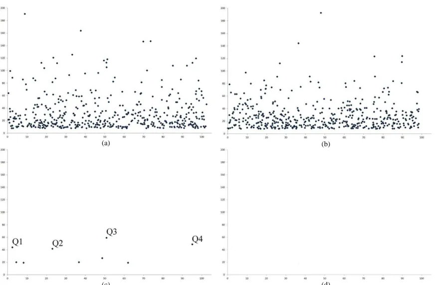
We also provided results for comparing GWAS in open-pollinated population and in inbred lines panel. An impressive result from GWAS with inbred lines panel is the efficacy of discarding spurious associations due to population structure (Figure 2). From the analysis of expansion volume, assuming a FDR of 1%, heritability of 0.8, and sample size 400 (simulation 1), the number of spurious associations in chromosome 3 (no QTL) were reduced from 477 to zero. Further, correcting for population structure decreased the number of significant associations in chromosome 1 (four QTL) from 464 to 9. This implies in a power of QTL detection of 100%, but three to five false-positive associations. The population structure analysis evidenced four subpopulations (Figure 3). In general, the efficacy of GWAS was greater with inbred lines panel (Table 3). The power of QTL detection was higher and the number of false-positive associations was lower. Further, in general only SNPs within the QTL showed significant associations. Notice also that no differences were observed between the traits and, similarly for open-pollinated populations, the analysis is ineffective assuming lower QTL effect and reduced heritability and sample size.

19

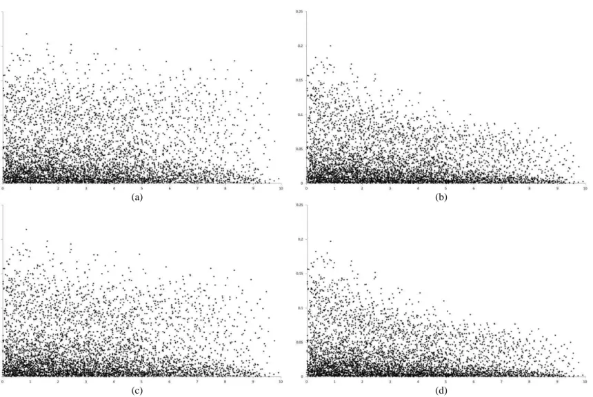
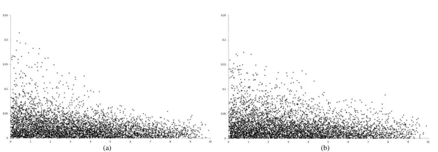
population 1, for example, the number of absolute LD values greater than 0.1 decreased 60%.

20 4. Discussion

4.1. GWAS in open-pollinated populations: theoretical aspects, potential and limitations

One of the main contributions of this research is to show the quantitative genetics theory for GWAS in open-pollinated populations. The theoretical aspects of quantitative genetics showed that considering there is no QTL in LD with one given SNP allele, the QTL identification can be based on a F-test where the null hypothesis is there is no difference between the SNP genotypic means of the individuals with different SNP genotypes from the population, or by a regression analysis to check if there is no relationship between the genotypic values of the individuals from the population and the number of copies of one given SNP allele. In both cases, it is clear that the QTL identification depends on the presence and the degree of LD between the QTL and the SNP locus.

21

causative polymorphisms. Additionally, causative polymorphisms for one trait may not necessarily be causal for another highly correlated trait (and, hence a spurious association), but will be statistically associated with both traits. Both of these types of false-positive associations do not occur randomly across the genome and thus, they are very challenging to eliminate.

The LD decay due to recombination after ten generations of random crosses was beneficial to QTL identification in population 1 – generation 10r. With around 25% decrease in LD, the GWAS was highly efficient, so the LD becomes restricted to the true QTL and one or few SNP loci very close or within the QTL. This situation implied in a good average power of QTL detection with lower false-positive associations and average bias in the QTL position than observed in population 1 – generation 0, disregarding the influence of population sample size, trait heritability and degree of dominance, and level of control of the type I error. These results are significantly comparable to those obtained by Yu et al. (2008) in a simulation study which investigated the genetic and statistical properties (average power of QTL detection, FDR and R2) of the nested association mapping (NAM) design currently being implemented in maize to dissect the genetic basis of complex quantitative traits. With 5,000 genotypes, these authors achieved 57% of average power of QTL detection (ranging from 30 to 85%), considering two trait heritabilities (0.4 and 0.7), two different numbers of QTL controlling the trait (20 and 50) and two different genotyping schemes (complete marker information and common-parent-specific markers only).

4.2. GWAS in open-pollinated populations: influence of QTL heritability and sample size

22

under evaluation (Yu et al. 2008). Importantly for genetic mapping applications, the heritability corresponds to the amount of phenotypic variation that can be attributed to genetic effects and thus to the cumulative effects of QTL (Buckler et al., 2009; Kump et al., 2011). High estimates of heritability depends on the quality of phenotypic data assessment, which results in genotypic values estimated with high accuracy and, consequently, should facilitate QTL detection with substantial power (Liu et al., 2011). The influence of QTL heritability on GWAS in open-pollinated populations was evidenced by the increase in power of QTL detection, associated with a little increase in the number of spurious associations and in the bias in QTL position. As in previous studies, a higher heritability always gave higher QTL detection power, particularly for QTL with moderate to small effect (Yu et al. 2008). Hung et al. (2012) assessed 19 quantitative traits in maize and achieved heritabilities greater than 0.8 for traits related to flowering time and plant architecture, resulting in a good power to detect QTL for these traits. In contrast, traits which had lower heritabilities (up to 0.6) and were more strongly affected by environmental variation allow only a reasonable power of QTL detection. Similar results were obtained by Kump et al. (2011), which evaluated resistance to southern leaf blight (SLB) disease in maize and obtained a heritability of 87%, indicating the potential for accurate mapping of SLB-resistance genes. These authors identified 32 QTL with predominantly small and additive effects on SLB resistance and many of the SNP within and outside of QTL intervals are also within or near to genes previously shown to be involved in plant disease resistance in other studies (Poland et al., 2009; Broglie et al., 2009).

23

population size necessarily increases the number of individuals with rare alleles, thus improving the power to test the association between these rare alleles and the trait of interest. The influence of population sample size on GWAS in our study was demonstrated with the increase in power of QTL detection, increase in the number of spurious associations (mainly in chromosomes with one to four QTL), and in the bias in QTL position, disregarding the trait, heritability and FDR. The increase in number of false-positive associations due to increase in population sample size was much more pronounced with high heritabilities (0.08 and 0.12) of each QTL. Yu et al. (2008) showed that the gain in accuracy by increasing sample size was evidenced by increased power of QTL detection and smaller FDR, mainly with heritability of 0.7 in comparison with a heritability of 0.4. Long & Langley (1999) performed a simulation study which demonstrated that sufficient power to detect marker-trait associations for QTL that account for as little as 5% of the phenotypic variation occurs when approximately 500 individuals are genotyped for approximately 20 SNP loci within the candidate gene region. These authors declared that more power is achieved by increasing the population size than by increasing the SNP density within the candidate gene.

24

increasing the heritability of each QTL (from 0.04 to 0.12) for low population sample size (200 individuals) or by increasing the control of type I error (from 5 to 1%) with high QTL heritabilities (0.08 and 0.12) and population sample size (400 individuals).

4.3. GWAS in open-pollinated populations, inbred lines panel and RILs

Most papers about GWAS with maize published until now have employed inbred lines panel (Samayoa et al., 2015; Van Inghelandt et al., 2012; Yang et al., 2010) or nested association mapping (NAM) populations (Bian et al., 2014; Tian et al., 2011; Kump et al., 2011) and almost no information on GWAS in open-pollinated populations was found in literature. According to Flint-Garcia et al. (2005), the inbred lines panel exploits the rapid breakdown of LD in diverse maize lines, enabling very high resolution for QTL mapping via association analysis. One of the most important maize inbred panel was assembled by Flint-Garcia et al. (2005) for association mapping and consists of 302 inbred lines from temperate and tropical regions, both current breeding lines and historically important lines, which represents a large fraction of the global genetic diversity in maize breeding (Yang et al., 2010). This population has been successfully used by the maize community to perform GWAS in economically important quantitative traits such as kernel composition (Cook et al., 2012) and Fusarium ear rot resistance (Zila et al., 2013).

25

efficiency of GWAS with inbred lines panel was significant, since the power of QTL detection was much higher than with open-pollinated population and RILs, associated with a lower number of false-positive associations (close to zero) and bias in the QTL position, disregarding the trait, heritability, population sample size and FDR. The lowest parametric LD values for the inbred lines panel are comparable to other studies already published (Yan et al., 2009; Remington et al., 2001). Moreover, with the inbred lines panel, in general only SNP loci within the QTL showed significant association, which is a highlighted result from GWAS that can serve as basis for a fine mapping strategy to be used in marker-assisted selection and map-based cloning genes (Gupta et al., 2005).

The most important example of a NAM population synthesized for GWAS is the set of 5,000 RILs derived from crosses between the reference maize inbred line B73 and 25 other founder inbreds. This maize NAM panel captures a substantial proportion of the global genetic diversity of maize inbred lines and the high allele diversity and large sample size provide a great power of QTL detection (McMullen et al., 2009; Kump et al., 2011). According to Yu et al. (2008), NAM populations have the advantages of lower sensitivity to genetic heterogeneity and higher power of QTL detection, as well as higher efficiency in using the genome sequence or dense markers while still maintaining high allele richness due to diverse founders. By choosing diverse founders, LD within chromosome segments resulting from historical/evolutionary recombination was mostly preserved in RILs due to the small probability of recombination within the short genetic distances between flanking common-parent-specific markers, which leads to a great power of QTL detection.

26

27 5. Conclusion

28 6. Acknowledgments

29 7. References

Azevedo, C. F.; Resende, M. D. V.; Silva, F. F.; Viana, J. M. S.; Valente, M. S. F.; Resende Jr., M. F. B.; Muñoz, P. (2015) Ridge, Lasso and Bayesian additive-dominance genomic models. BMC Genetics, 16:105-118. doi 10.1186/s12863-015-0264-2

Barendse, W.; Reverter, A.; Bunch, R. J.; Harrison, B. E.; Barris, W.; Thomas, M. B. (2007) A validated whole-genome association study of efficient food conversion in cattle. Genetics, 176:1893-905.

Benjamini, Y.; Hochberg, Y. (1995) Controlling the false discovery rate: a practical and powerful approach to multiple testing. Journal of the Royal Statistical Society, 57:289-300.

Bian, Y.; Yang, Q.; Balint-Kurti, P. J.; Wisser, R. J.; Holland, J. B. (2014) Limits on the reproducibility of marker associations with southern leaf blight resistance in the maize nested association mapping population. BMC Genomics, 15:1068-1082.

Bolormaa, S.; Hayes, B.; Savin, K.; Hawken, R.; Barendse, W.; Arthur, P.; et al. (2011) Genome-wide association studies for feedlot and growth traits in cattle. Journal of Animal Science, 89:1684-1697.

Bradbury, P. J.; Zhang, Z.; Kroon, D. E.; Casstevens, T. M.; Ramdoss, Y.; Buckler, E. S. (2007) TASSEL: software for association mapping of complex traits in diverse samples. Bioinformatics, 23(19):2633-2635. doi 10.1093/bioinformatics/btm308 Broglie, K. E.; Butler, K. H.; Butruille, M. G.; Conceição, A. S.; Frey, T. J.; Hawk, J. A.;

30

Buckler, E. S.; Holland, J. B.; Bradbury, P. J.; Acharya, C. B.; Brown, P. J.; Browne, C.; Ersoz, E.; Flint-Garcia, S. A.; Garcia, A.; Glaubitz, J. C.; Goodman, M. M.; Harjes, C.; Guill, K.; Kroon, D. E.; Larsson, S.; Lepak, N. K.; Li, H. H.; Mitchell, S. E.; Pressoir, G.; Peiffer, J. A.; Rosas, M. O.; Rocheford, T. R.; Romay, M. C.; Romero, S.; Salvo, S.; Villeda, H. S.; da Silva, H. S.; Sun, Q.; Tian, F.; Upadyayula, N.; Ware, D.; Yates, H.; Yu, J. M.; Zhang, Z. W.; Kresovich, S.; McMullen, M. D. (2009) The genetic architecture of maize flowering time. Science, 325:714-718.

Cockerham, C. C. (1954) An extension of the concept of partitioning hereditary variance for analysis of covariance among relatives when epistasis is present. Genetics, 39:859-882.

Cook, J. P.; McMullen, M. D.; Holland, J. B.; Tian, F.; Bradbury, P.; Ross-Ibarra, J.; Buckler, E. S.; Flint-Garcia, S. A. (2012) Genetic Architecture of Maize Kernel Composition in the Nested Association Mapping and Inbred Association Panels. Plant Physiology, 158:824-834.

Corder, E. H.; Saunders, A. M.; Risch, N. J.; Strittmatter, W. J.; Schmechel, D. E.; et al. (1994) Protective effect of apolipoprotein-E type-2 allele for late-onset Alzheimer-disease. Nature Genetics, 7:180-184.

Falush, D.; Stephens, M.; Pritchard, J. K. (2003) Inference of population structure using multilocus genotype data: linked loci and correlated allele frequencies. Genetics, 164:1567-1587.

31

Flint-Garcia, S. A.; Thornsberry, J. M.; Buckler, E. S. (2003) Structure of linkage disequilibrium in plants. Annual Reviews of Plant Biology, 54:357-374. doi 10.1146/annurev.arplant.54.031902.134907

Flint-Garcia, S. A.; Thuillet, A. C.; Yu, J.; Pressoir, G.; Romero, S. M.; Mitchell, S. E.; Doebley, J.; Kresovich, S.; Goodman, M. M.; Buckler, E. S. (2005) Maize association population: a high-resolution platform for quantitative trait locus dissection. The Plant Journal, 44:1054-1064. doi 10.1111/j.1365-313X.2005.02591.x

Fuller, W. A.; Gallant, A. R. (1974) Fitting segmented polynomial regression models whose join points have to be estimated. Journal of American Statistician Association, 68:144-147.

Gouy, M.; Rousselle, Y.; Thong Chane, A.; Anglade, A.; Royaert, S.; Nibouche, S.; Costet, L. (2015) Genome wide association mapping of agro-morphological and disease resistance traits in sugarcane. Euphytica, 202(2):269-284. doi 10.1007/s10681-014-1294-y

Gupta, P. K.; Rustgi, S.; Kulwal, P. L. (2005) Linkage disequilibrium and association studies in higher plants: present status and future prospects. Plant Molecular Biology, 57:461-485. doi 10.1007/s11103-005-0257-z

Hastbacka, J.; de la Chapelle, A.; Kaitila, I.; Sistonen, P.; Weaver, A.; Lander, E. (1992) Linkage disequilibrium mapping in isolated founder populations: diastrophic dysplasia in Finland. Nature Genetics, 2:204-211.

Hill, W. G.; Robertson, A. (1968) Linkage disequilibrium in finite populations. Theoretical and Applied Genetics, 38(6):226-231. doi 10.1007/BF01245622

32

Genome-wide association study of Arabidopsis thaliana leaf microbial community. Nature Communications, 5:5320-5326. doi 10.1038/ncomms6320

Hung, H. Y.; Browne, C.; Guill, K.; Coles, N.; Eller, M.; Garcia, A.; Lepak, N.; Melia-Hancock, S.; Oropeza-Rosas, M.; Salvo, S.; Upadyayula, N.; Buckler, E. S.; Flint-Garcia, S. A.; McMullen, M. D.; Rocheford, T. R.; Holland, J. B. (2012) The relationship between parental genetic or phenotypic divergence and progeny variation in the maize nested association mapping population. Heredity, 108:490-499.

Kempthorne, D. (1957) An introduction to genetic statistics. John Wiley & Sons Inc, New York.

Kerem, B. S.; Rommens, J. M.; Buchanan, J. A.; Markiewicz, D.; Cox, T. K.; et al. (1989) Identification of the cystic fibrosis gene: genetic analysis. Science, 245:1073-1080. Kijas, J. W.; Townley, D.; Dalrymple, B. P.; Heaton, M. P.; Maddox, J. F.; McGrath, A.;

et al. (2009) A genome wide survey of SNP variation reveals the genetic structure of sheep breeds. PLoS One, 4:e4668.

Krill, A. M.; Kirst, M.; Kochian, L. V.; Buckler, E. S.; Hoekenga, O. A. (2010) Association and linkage analysis of aluminum tolerance genes in maize. PLoS One, 5(4):e9958.

Kump, K. L.; Bradbury, P. J.; Wisser, R. J.; Buckler, E. S.; Belcher, A. R.; Oropeza-Rosas, M. A.; Zwonitzer, J. C.; Kresovich, S.; McMullen, M. D.; Ware, D.; Balint-Kurti, P. J.; Holland, J. B. (2011) Genome-wide association study of quantitative resistance to southern leaf blight in the maize nested association mapping population. Nature Genetics, 43(2):163-169. doi:10.1038/ng.747

33

Li, C.; Li, Y.; Bradbury, P. J.; Wu, X.; Shi, Y.; Song, Y.; Zhang, D.; Rodgers-Melnick, E.; Buckler, E. S.; Zhang, Z.; Li, Y.; Wang, T. (2015) Construction of high-quality recombination maps with low-coverage genomic sequencing for joint linkage analysis in maize. BMC Biology, 13:78-89. doi 10.1186/s12915-015-0187-4

Li, F.; Chen, B.; Xu, K.; Wu, J.; Song, W.; Bancroft, I.; Harper, A. L.; Trick, M.; Liu, S.; Gao, G.; Wang, N.; Yan, G.; Qiao, J.; Li, J.; Li, H.; Xiao, X.; Zhang, T.; Wu, X. (2014) Genome-wide association study dissects the genetic architecture of seed weight and seed quality in rapeseed (Brassica napus L.). DNA Research, 1:1-13. doi 10.1093/dnares/dsu002

Liu, K.; Muse, S. V. (2005) PowerMarker: integrated analysis environment for genetic marker data. Bioinformatics, 21:2128-2129.

Liu, W.; Gowda, M.; Steinhoff, J.; Maurer, H. P.; Wurschum, T.; Longin, C. F. H.; Cossic, F.; Reif, J. C. (2011) Association mapping in an elite maize breeding population. Theoretical and Applied Genetics, 123:847-858. doi 10.1007/s00122-011-1631-7 Long, A. D.; Langley, C. H. (1999) The power of association studies to detect the

contribution of candidate genetic loci to variation in complex traits. Genome Research. 9: 720-731.

Lu, Y.; Zhang, S.; Shah, T.; Xie, C.; Hao, Z.; Li, X.; Farkhari, M.; Ribaut, J. M.; Cao, M.; Rong, T.; Xu, Y. (2010) Joint linkage-linkage disequilibrium mapping is a powerful approach to detecting quantitative trait loci underlying drought tolerance in maize. PNAS, 107(45):19585-19590. doi 10.1073/pnas.1006105107

34

hexaploid spring wheat (Triticum aestivum L.). G3: Genes, Genomes & Genetics, 5:449-465. doi 10.1534/g3.114.014563

McMullen, M. D.; Kresovich, S.; Villeda, H. S.; Bradbury, P.; Li, H.; Sun, Q.; Flint-Garcia, S. A.; Thornsberry, J.; Acharya, C.; Bottoms, C.; Brown, P.; Browne, C.; Eller, M.; Guill, K.; Harjes, C.; Kroon, D.; Lepak, N.; Mitchell, S. E.; Peterson, B.; Pressoir, G.; Romero, S.; Oropeza-Rosas, M.; Salvo, S.; Yates, H.; Hanson, M.; Jones, E.; Smith, S.; Glaubitz, J. C.; Goodman, M.; Ware, D.; Holland, J. B.; Buckler, E. S. (2009) Genetic properties of the maize nested association mapping population. Science, 325(5941):737-740. doi: 10.1126/science.1174320

Morris, G. P.; Ramub, P.; Deshpandeb, S. P.; Hashc, C. T.; Shahb, T.; Upadhyayab, H. D.; Riera-Lizarazub, O.; Brownd, P. J.; Acharyae, C. B.; Mitchelle, S. E.; Harrimane, J.; Glaubitze, J. C.; Buckler, E. S.; Kresovicha, S. (2013) Population genomic and genome-wide association studies of agro climatic traits in sorghum. PNAS, 110(2):453-458. doi 10.1073/pnas.1215985110

Nordborg, M.; Borevitz, J. O.; Bergelson, J.; Berry, C. C.; Chory, J.; et al. (2002) The extent of linkage disequilibrium in Arabidopsis thaliana. Nature Genetics, 30:190-193. Pace, J.; Gardner, C.; Romay, C.; Ganapathysubramanian, B.; Lübberstedt, T. (2015) Genome-wide association analysis of seedling root development in maize (Zea mays L.). BMC Genomics, 16:47-58. doi 10.1186/s12864-015-1226-9

Pasam, R. K.; Sharma, R.; Malosetti, M.; van Eeuwijk, F. A.; Haseneyer, G.; Kilian, B.; Graner, A. (2012) Genome-wide association studies for agronomical traits in a worldwide spring barley collection. BMC Plant Biology, 12:16-37.

35

Pritchard, J. K.; Stephens, M.; Donnelly, P. (2000) Inference of population structure using multilocus genotype data. Genetics, 155:945-959.

Remington, D. L.; Thornsberry, J. M.; Matsuoka, Y.; Wilson, L. M.; Whitt, S. R.; Doebley, J.; Kresovich, S.; Goodman, M. M.; Buckler, E. S. (2001) Structure of linkage disequilibrium and phenotypic associations in the maize genome. PNAS, 98(20):11479-11484. doi 10.1073ypnas.201394398

Risch, N.; Merkangas, K. (1996) The future of genetic studies of complex human diseases. Science, 273(5281):1516-1517.

Samayoa, L. F.; Malvar, R. A.; Olukolu, B. A.; Holland, J. B.; Butrón, A. (2015) Genome-wide association study reveals a set of genes associated with resistance to the Mediterranean corn borer (Sesamia nonagrioides L.) in a maize diversity panel. BMC Plant Biology, 15:35-49. doi 10.1186/s12870-014-0403-3

SAS Institute (2007) The SAS System for Windows, version 9.2. SAS Institute Inc., Cary NC.

Schaefer, C. M.; Bernardo, R. (2013) Genome-wide association mapping of flowering time, kernel composition, and disease resistance in historical Minnesota maize inbreds. Crop Science, 53:2518-2529. doi 10.2135/cropsci2013.02.0121

Sladek, R.; Rocheleau, G.; Rung, J.; Dina, C.; Shen, L.; Serre, D.; et al. (2007) A genome-wide association study identifies novel risk loci for type 2 diabetes. Nature, 445:881-885.

Stuber, C. W.; Polacco, M.; Senior, M. L. (1999) Synergy of empirical breeding, marker assisted selection and genomics to increase crop yield potential. Crop Science, 39:1571-1583.

36

in maize. Theoretical and Applied Genetics, 128:851-864. doi 10.1007/s00122-015-2475-3

Thirunavukkarasu1, N.; Hossain, F.; Arora, K.; Sharma, R.; Shiriga, K.; Mittal, S.; Mohan, S.; Namratha, P. M.; Dogga, S.; Rani, T. S.; Katragadda, S.; Rathore, A.; Shah, T.; Mohapatra, T.; Gupta, H. S. (2014) Functional mechanisms of drought tolerance in subtropical maize (Zea mays L.) identified using genome-wide association mapping. BMC Genomics, 15:1182-1193.

Thornsberry, J. M.; Goodman, M. M.; Doebley, J.; Kresovich, S.; Nielsen, D.; et al. (2001) Dwarf8 polymorphisms associate with variation in flowering time. Nature Genetics, 28:286-289.

Tian, F.; Bradbury, P. J.; Brown, P. J.; Hung, H.; Sun, Q.; Flint-Garcia, S. A.; et al. (2011) Genome-wide association study of leaf architecture in the maize nested association mapping population. Nature Genetics, 43:159-162.

Van Inghelandt, D.; Melchinger, A. E.; Martinant, J. P.; Stich, B. (2012) Genome-wide association mapping of flowering time and northern corn leaf blight (Setosphaeria turcica) resistance in a vast commercial maize germplasm set. BMC Plant Biology, 12:56-70.

Viana, J. M. S.; Valente, M. S. F.; Silva, F. F.; Mundim, G. B.; Paes, G. P. (2013) Efficacy of population structure analysis with breeding populations and inbred lines. Genetica, 141:389-399. doi 10.1007/s10709-013-9738-1

Weir, B. (2010) Statistical genetic issues for genome-wide association studies. Genome, 53:869-875. doi 10.1139/G10-062

37

Wu, R.; Zeng, Z. B. (2001) Joint linkage and linkage disequilibrium mapping in natural populations. Genetics, 157:899-909.

Yan, J. B.; Shah, T.; Warburton, M.; Buckler, E. S.; McMullen, M. D.; Crouch, J. (2009) Genetic characterization of a global maize collection using SNP markers. PLoS ONE 4:e8451.

Yang, W.; Guo, Z.; Huang, C.; Wang, K.; Jiang, N.; Feng, H.; Chen, G.; Liu, Q.; Xiong, L. (2015) Genome-wide association study of rice (Oryza sativa L.) leaf traits with a high-throughput leaf scorer. Journal of Experimental Botany, 66(18):5605-5615. doi 10.1093/jxb/erv100

Yang, X.; Yan, J.; Shah, T.; Warbuton, M. L.; Li, Q.; Li, L.; Gao, Y.; Chai, Y.; Fu, Z.; Zhou, Y.; Xu, S.; Bai, G.; Meng, Y.; Zheng, Y.; Li, J. (2010) Genetic analysis and characterization of a new maize association mapping panel for quantitative trait loci dissection. Theoretical and Applied Genetics, 121:417-431. doi 10.1007/s00122-010-1320-y

Yu, J. M.; Buckler, E. S. (2006) Genetic association mapping and genome organization of maize. Current Opinion in Biotechnology, 17:1-6.

Yu, J.; Holland, J. B.; McMullen, M. D.; Buckler, E. S. (2008) Genetic design and statistical power of nested association mapping in maize. Genetics, 178:539-551. doi 10.1534/genetics.107.074245

38

39

Table 1 Average number of significant associations with a FDR of 1 and 5%, power of QTL detection (%), number of false-positive associations in chromosomes with no QTL and one to four QTL, bias in the QTL position (cM), and average range for the regions with identified QTL, regarding population 1, generation 10r (random cross), three traits (expansion volume (EV; mL/g), grain yield (GY; g/plant), and days to maturity (DM)), two sample sizes, and two heritabilities1

40

Table 2 Average number of significant associations with a FDR of 1 and 5%, power of QTL detection (%), number of false-positive associations in chromosomes with no QTL and one to two QTL, bias in the QTL position (cM), and average range for the regions with identified QTL, regarding population 1, generation 10r (random cross), three traits (expansion volume (EV; mL/g), grain yield (GY; g/plant), and days to maturity (DM)), two sample sizes, and QTL heritability of 12%1

Population FDR Trait Sample Sig. Assoc. Power False+0 False+1-2 Bias Av. range

41

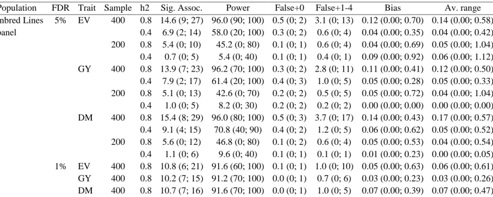
Table 3 Average number of significant associations with a FDR of 1 and 5%, power of QTL detection (%), number of false-positive associations in chromosomes with no QTL and one to four QTL, bias in the QTL position (cM), and average range for the regions with identified QTL, regarding an inbred lines panel, three traits (expansion volume (EV; mL/g), grain yield (GY; g/plant), and days to maturity (DM)), two sample sizes, and two heritabilities1

42

Table 4 Average number of significant associations with a FDR of 1 and 5%, power of QTL detection (%), number of false-positive associations in chromosomes with no QTL and one to four QTL, bias in the QTL position (cM), and average range for the regions with identified QTL, regarding population 1, generation 10r10s (random cross and selfing), three traits (expansion volume (EV; mL/g), grain yield (GY; g/plant), and days to maturity (DM)), two sample sizes, and two heritabilities1

Population FDR Trait Sample h2 Sig. Assoc. Power False+0 False+1-4 Bias Av. range RILs 1% EV 400 0.8 34.5 (4; 122) 87.0 (40; 100) 0.3 (0; 2) 12.7 (0; 68) 0.61 (0.00; 1.05) 0.90 (0.00; 2.43)

43

(a) (b)

(c) (d)

44

(a) _(b)

(c) (d)

45

(a) (b)

46

(a) (b)

(c) (d)

47

(a) (b)

(c) (d)

48

(a) (b)