www.atmos-meas-tech.net/10/167/2017/ doi:10.5194/amt-10-167-2017
© Author(s) 2017. CC Attribution 3.0 License.
Altitude registration of limb-scattered radiation
Leslie Moy1, Pawan K. Bhartia2, Glen Jaross2, Robert Loughman3, Natalya Kramarova1, Zhong Chen1, Ghassan Taha4, Grace Chen1, and Philippe Xu5
1Science Systems and Applications, Inc. (SSAI), 10210 Greenbelt Road, Suite 600, Lanham, Maryland 20706, USA 2NASA Goddard Space Flight Center, Greenbelt, Maryland, USA
3Hampton University, Hampton, Virginia, USA 4GESTAR, Columbia, Maryland, USA
5Science Applications International Corporation (SAIC), Lanham, Maryland, USA Correspondence to:Leslie Moy ([email protected])
Received: 28 March 2016 – Published in Atmos. Meas. Tech. Discuss.: 8 June 2016 Revised: 30 November 2016 – Accepted: 19 December 2016 – Published: 12 January 2017
Abstract. One of the largest constraints to the retrieval of accurate ozone profiles from UV backscatter limb sounding sensors is altitude registration. Two methods, the Rayleigh scattering attitude sensing (RSAS) and absolute radiance residual method (ARRM), are able to determine altitude reg-istration to the accuracy necessary for long-term ozone mon-itoring. The methods compare model calculations of radi-ances to measured radiradi-ances and are independent of onboard tracking devices. RSAS determines absolute altitude errors, but, because the method is susceptible to aerosol interfer-ence, it is limited to latitudes and time periods with mini-mal aerosol contamination. ARRM, a new technique intro-duced in this paper, can be applied across all seasons and altitudes. However, it is only appropriate for relative alti-tude error estimates. The application of RSAS to Limb filer (LP) measurements from the Ozone Mapping and Pro-filer Suite (OMPS) on board the Suomi NPP (SNPP) satellite indicates tangent height (TH) errors greater than 1 km with an absolute accuracy of±200 m. Results using ARRM indi-cate a ∼300 to 400 m intra-orbital TH change varying sea-sonally±100 m, likely due to either errors in the spacecraft pointing or in the geopotential height (GPH) data that we use in our analysis. ARRM shows a change of∼200 m over
∼5 years with a relative accuracy (a long-term accuracy) of
±100 m outside the polar regions.
1 Introduction
Instruments that measure the solar radiation scattered by the Earth’s atmosphere in the limb direction provide a low-cost way of measuring trace gases, aerosol profiles, and clouds from satellites. The technique can provide daily full cov-erage of the sunlit Earth from commonly used polar sun-synchronous satellites. To meet long-term ozone monitoring needs (3 % precision between 15 and 50 km) requires the al-titude registration of the radiances to be accurate to within
∼100 m (Jaross et al., 2014). For a sensor orbiting at 800 km, this translates into∼6 arcsec accuracy in the pointing direc-tion of the instrument line of sight (LOS) with respect to Earth’s horizon. This is often a difficult goal to achieve.
In this paper we critically examine the performance of two methods of altitude registration that compare measured and simulated radiances. We discuss the inherent strengths and limitations of each method and then assess their perfor-mance using data from the Ozone Mapping and Profiler Suite (OMPS) Limb Profiler (LP), launched on board the Suomi NPP (SNPP) satellite on 28 October 2011.
near 3 hPa (∼40 km). Since aerosol contamination limits the range of latitudes and times where RSAS can be applied, we developed the absolute radiance residual method (ARRM). ARRM excels in relative rather than absolute limb altitude registration.
We describe the theoretical basis of these two techniques in Sect. 2 and their application to the OMPS LP instrument in Sect. 3. We present several validations of our uncertainty estimates in Sect. 4 and summarize our findings in Sect. 5.
2 Theoretical basis
Most scene-based altitude registration methods applied to limb-scattering instruments take advantage of the fact that the atmospheric Rayleigh scattering measured by these in-struments varies by 12–14 % km−1. For wavelengths longer
than 310 nm, the limb-scattered (LS) radiance has a signif-icant contribution from diffuse upwelling radiance (DUR), which is affected by tropospheric clouds, aerosols, and sur-face albedos within a circular cone whose base extends hun-dreds of kilometers to the horizon. The further these reflec-tors are from the apex of the cone, the less is their contribu-tion to DUR. At non-ozone-absorbing wavelengths DUR can be as much as half of the measured radiance. Since DUR is challenging to model accurately, all successful altitude regis-tration methods must be relatively insensitive to reflectivity variations within the cone.
The RSAS method, described in Sect. 2.1, employs signal ratios in which the DUR effects largely cancel. ARRM, de-scribed in Sect. 2.2, uses 295 nm radiances for which ozone absorption screens the DUR signal. The knee method, de-scribed in Sect. 2.3, has been used extensively by others (Sioris et al., 2003; Kaiser et al., 2004; Rault, 2005; von Sav-igny et al., 2005; Taha et al., 2008), but our analysis indicates that it offers no advantages over RSAS and ARRM.
2.1 Rayleigh scattering attitude sensor (RSAS) method
This technique is named after the sensor that was flown on the Space Shuttle STS-72 in January 1996 (Janz et al., 1996) to test a concept originally proposed by Bhartia in 1992. The technique takes advantage of the fact that the gradient in the log of the LS radiance I with altitude z, dlnI/dz, changes by a factor of 3 between 40 and 20 km for wave-lengths near 350 nm (Fig. 1). This is caused by the exponen-tially increasing attenuation of Rayleigh scattering with pres-sure. At 40 km this attenuation is small, and when aerosol loading is minimal, dlnI/dz is largely determined by dlnP/dz, whereP is the atmospheric pressure at altitudez. However, at 20 km the extinction and scattering at 350 nm are nearly equal, which means limb radiances from this altitude are rel-atively insensitive to the exact altitude of the tangent point. The tangent point is where the sensor line of sight (LOS) in-tersects the Earth radius vector at a right angle. Though
sev-0 4 8 10
(z)/Ic(40km)
0 10 20 30 40
al
ti
tude
,k
m
-0.15 -0.10 -0.05 0.00 0.05 d(lnIc)/dz
0 10 20 30 40
al
ti
tude
,k
m
A
l#t
ude
(k
m
)
Al
#
tu
d
e
(km
)
40km C
C (unitless) 6 2
C
I (z)/I d(lnI )/dz (%/km)
-15 -10 -5 0 5
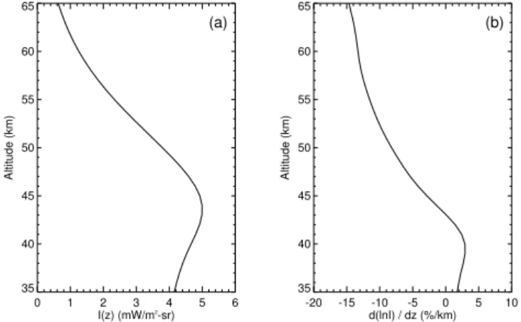
Figure 1.Left panel shows calculated 350 nm radiances as a
func-tion of altitude, normalized at 40.5 km. The GSLS calculafunc-tion mod-els the OMPS LP field of view without aerosols. The shape of the curve originates from the competition between molecular scatter-ing, which increases roughly linearly with pressure, and attenuation, which becomes important when the Rayleigh optical thicknesses near the tangent point start to become large. Attenuation causes the slope of 350 nm radiances to change sharply between 40 and 20 km (right panel), a∼10 % km−1difference between 20 and 40 km. The slope is used to estimate altitude registration errors by comparing measured ratios with model simulated ratios.
eral variations of the RSAS technique have been developed for ozone sensors (McPeters et al., 2000; Rault, 2005; Taha et al., 2008), we find that the simplest formulation described below works as well as any other.
Ifris the ratio of radiances for wavelengthλat altitudesz1
andz2, ands1ands2are the vertical slopes dlnI/dzat those
altitudes, then the error in tangent height (TH) can be calcu-lated as follows:
1z= −ln(r)m−ln(r)c
s (z1)−s (z2)
, (1)
where the subscript “m” refers to the measured radiance ra-tios, and “c” refers to the ratio calculated using a radiative transfer model. To get the most accurate estimate of TH error, the denominator should be as large as possible, and the un-certainties in estimating the numerator should be small. The smallest uncertainties in the numerator occur at wavelengths near 350 nm, where trace gas absorption and aerosol scatter-ing effects are small. Settscatter-ingz1to be near 40 km andz2to be at or below 20 km maximizes the value of the denominator, typically near 0.10 km−1. An accuracy of 0.01 (equal to 1 %
in radiance ratios) is therefore needed to estimate TH within 100 m.
-70 -60 -50 -40 -30 -20 -10 0 10 20 30 40 50 60 70 Latitude (deg)
10 15 20 25
Radiance (mW / m
2-sr)
40.5 km
20.5 km
Figure 2.The 350 nm sun-normalized radiances from one orbit of
OMPS LP (center slit) taken on 2 February 2012. The blue line shows 40.5 km values, and the green line shows 20.5 km values (di-vided by 8 to put both curves on a similar scale) versus latitude. Since the global aerosol loading on this day was small, the short-scale features in both curves are largely caused by variations in cloud and surface albedo. The 20.5 km curve has sharper features and appears to be shifted toward the South Pole. This is because large Rayleigh attenuation at 20.5 km causes the radiances to have much higher sensitivity to the atmosphere on the satellite side of the tangent point (TP), while 40.5 km radiances have similar sen-sitivities to both sides. This effect creates large noise in applying the RSAS technique to orbital data. However, since the noise varies randomly from orbit to orbit, it can be reduced by averaging data from multiple orbits.
toward the South Pole. This is because large Rayleigh atten-uation at 20.5 km causes the radiances to have much higher sensitivity to the atmosphere on the satellite side of the tan-gent point (TP), while the 40.5 km radiances have similar sensitivities to both sides. This effect creates large noise in applying the RSAS technique to orbital data. However, since the noise varies randomly from orbit to orbit, DUR model-ing errors are reduced by averagmodel-ing data from multiple orbits (this is confirmed in daily averages of the sun-normalized ra-diances where short-scale features are not seen).
Aerosols in the instrument’s LOS are a more significant source of error for the RSAS method. Though the effect of aerosols near 350 nm is small compared to longer wave-lengths, it is difficult to model due to subtle differences be-tween two large effects: the reduction of Rayleigh scatter-ing by aerosol extinction and the enhancement of limb ra-diances by aerosol scattering. Figure 3 shows the ratio of 350 nm limb-scattered radiances at 20.5 km with and with-out aerosols as a function of latitude. The strong latitude dependence is caused by an order-of-magnitude change in the aerosol scattering phase function with latitude com-bined with the attenuation of Rayleigh-scattered radiation by aerosols along the LOS. In the Southern Hemisphere, where LP measures backscattered radiation, the latter effect domi-nates and the radiation decreases. The net effect is difficult
-70 -60 -50 -40 -30 -20 -10 0 10 20 30 40 50 60 70
Latitude (deg) 0.5
1.0 1.5 2.0
Radiance ratio (unitless)
-70 -60 -50 -40 -30 -20 -10 0 10 20 30 40 50 60 70
Latitude (deg)
0 20 40 60 80 100 120 140 160 180
Single scattering angle at 25 km TH (deg)
Figure 3.The GSLS-modeled ratio of 350 nm limb-scattered
radi-ances at 20.5 km with and without aerosols (left axis) and single-scattering angle (right axis) as a function of latitude. A nominal latitude-independent aerosol extinction profile was used in the cal-culation for the OMPS LP viewing geometry on 2 February 2012. The strong latitude dependence is caused by an order of magnitude change in aerosol scattering phase function with latitude combined with the attenuation of Rayleigh-scattered radiation by aerosols along the line of sight (LOS). In the Southern Hemisphere, where LP measures aerosols in the backscatter direction, the latter effect dominates and the radiation decreases. The net effect is very sensi-tive to altitude, variation of aerosol extinction profile along the LOS, and aerosol particle size distribution, and it is therefore difficult to calculate accurately.
to calculate accurately since it is very sensitive to aerosol altitude, variation of the aerosol extinction profile along the LOS, and aerosol particle size distribution. Model calcula-tions with and without an average loading of aerosols er-roneously attribute TH errors of ∼100 m in the Southern Hemisphere and∼200 m in the Northern Hemisphere.
Though the effect of aerosols is similar to the cloud effect mentioned earlier, it is not random because aerosols tend to have systematic latitudinal variability at these altitudes we consider. Given this complexity, the RSAS method works best in latitudes and months where the 350 nm aerosol ex-tinction at 20 km is relatively small.
Another potential source of uncertainty in applying the RSAS technique comes from uncertainty in simulating ra-diances at 40 km; one needs to have accurate pressure pro-files for altitudes at and above 40 km. If the pressure propro-files are obtained from GPH profiles provided by meteorological data assimilation systems, a one-to-one relationship exists between the two errors: a 100 m error in GPH at 3 hPa trans-lates into∼100 m error in determining TH altitude. RSAS is not sensitive to GPH errors that are independent of altitude. 2.2 Absolute radiance residual method (ARRM)
clouds (PMCs), the atmosphere is typically free of particulate matter at 65 km. PMCs, which form in the polar summer and are typically located at 80 km, can significantly affect 65 km limb radiances if they are in the LOS of the instrument. For-tunately most of the PMC contamination is screened using a 350 nm channel radiance residual flag at 65 km.
Though 295 nm radiances can be very ozone sensitive, this sensitivity drops to less than 0.2 % for a 10 % change in ozone above 65 km because the ozone density at high alti-tudes is exceedingly low. At this altitude the ozone concen-tration typically changes by 25 % per kilometer, so model radiance errors will be within 0.5 % provided the OMPS TH is accurate to 1 km.
A difficulty in applying ARRM is the inaccuracy of GPH data near 0.1 hPa needed to calculate 295 nm radiances at 65 km. GPH uncertainty increases with increased altitude (Schwartz et al., 2008). To reduce the effect of GPH inac-curacies, we developed a variation of a technique that has been used for many years to derive mesospheric temperature profiles from the vertical slope of Rayleigh-scattered radi-ances measured by ground-based UV lidars (McGee et al., 1991). The technique described in their paper computes tem-peratures using the relative density differences between suc-cessive altitudes where the scattering mechanism is purely Rayleigh. Since we rely on the same region of Rayleigh dom-inance, we can apply their technique to correct for errors in the GPH assumptions. GPH is related to temperature by as-suming hydrostatic balance. The 350 and 295 nm residuals are affected similarly by the errors in the GPH with altitude, so we use the 350 nm residual to correct for the GPH errors at 295 nm. To the extent that stray light is also wavelength independent, this correction will remove stray-light errors.
The residual at wavelengthλat altitudez, defined as d(λ,
z)=lnIm(λ,z)−lnIc(λ,z), is corrected using 350 nm
resid-uals:
dcorr(λ, z)=d(λ, z)−[d(350, z)−d(350, z0)], (2)
wherez0is a normalization altitude.
The 350 nm differential residuals on the right side of Eq. (2) provide an estimate of the relative error in calculat-ing radiances uscalculat-ing meteorological data betweenzandz0. In effect we are limiting our sensitivity to GPH errors at 65 km by shifting our reliance on GPH assumptions to 40 km. Since GPH error is wavelength independent, we can use this term to correct the residuals at any wavelength, assuming that the meteorological data at z0 are accurate and that the 350 nm
wavelength is well calibrated versus altitude. The large re-sponse of OMPS LP at 350 nm results in signals that are the least affected by out-of-band stray light.
The TH error estimated using this method is given by
1z= dcorr(λ, z)
s(λ, z)−[s(350, z)−s (350, z0)]. (3)
To summarize, in the application of ARRM we use 295 nm radiance residuals at 65 km, adjusted with 350 nm differential
0 1 2 3 4 5 6
I(z) (mW/m2
-sr) 35
40 45 50 55 60 65
Altitude (km)
(a)
-20 -15 -10 -5 0 5 10
d(lnI) / dz (%/km) 35
40 45 50 55 60 65
Altitude (km)
(b)
Figure 4. (a)shows GSLS-model-calculated 305 nm radiances as
a function of altitude assuming an atmosphere with no aerosols. The slope(b)is caused by competition between Rayleigh scatter-ing and ozone absorption near the altitude of maximum radiance,
∼44 km. Above 55 km the sensitivity is nearly constant in height,
∼14 % km−1at 65 km. Above the knee the radiances decrease with altitude due to the exponential decrease in Rayleigh scattering and ozone density. Below the knee the ozone absorption becomes so large that it essentially blocks most of the Rayleigh-scattered radia-tion from reaching the satellite, making the radiances insensitive to atmospheric pressure. This characteristic knee shape allows one to estimate altitude registration error in a manner very similar to that of RSAS, but it also makes it is very susceptible to ozone profile assumptions, as illustrated in Fig. 5.
residuals. The choice of a wavelength shorter than 300 nm minimizes sensitivity to ozone profile and DUR modeling. Though it is best to setz0 as low as possible to minimize
GPH-caused errors, aerosol contamination limits it to around 40 km.
ARRM has two primary drawbacks. ARRM uses 350 nm differential residuals to correct for GPH errors between 40 and 65 km, so like RSAS this method is sensitive to er-rors in GPH profiles near 3 hPa. To the extent these erer-rors are time-invariant, ARRM works best to monitor changes in the TH error. ARRM is also sensitive to instrument calibration: a 1 % error in radiance calibration at 65 km produces∼70 m of error in determining the TH. It is therefore important that instrument calibration drifts are understood and corrected.
2.3 “Knee method”
of RSAS. An advantage of this method is the ability to use shorter wavelengths that are less sensitive to aerosols.
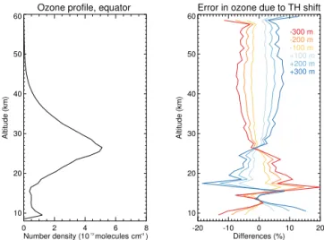
A disadvantage is the method requires accurate ozone and pressure profiles near and above the knee region. A rough es-timate of the ozone profile error caused by a TH error can be determined by simply shifting an ozone profile up and down (Fig. 5). From this analysis, errors in the ozone profile are found to be within 8 % at 40 km from TH errors of 300 m. It is important to note that the shift of the ozone profile does not necessarily translate to the exact error in altitude registration for limb radiances due to the nonlinearity of the inversion, which is especially important below 20 km. Differences of 8 % between the various ozone profile measurements are not unusual, and this will directly translate to uncertainty in the knee method.
The method also has a sensitivity to GPH errors that are similar to RSAS and ARRM. In our view this method pro-vides no compelling advantage over a direct comparison be-tween the limb ozone profile and a truth profile. Indeed, di-rect ozone comparisons are simpler and more reliable if the altitude registration error is the largest error source, and we use this technique to evaluate the results of RSAS and ARRM in Sect. 4.
3 Results
In this section we discuss altitude registration errors for the OMPS LP. Shortly after launch, RSAS analysis indicated a ∼2 km TH mis-registration, prompting an evaluation of pointing changes internal to the sensor. This evaluation re-lies on the image of the slit at the focal plane. Its description in Sect. 3.1 is included for completeness in describing the OMPS LP TH registration determination but is not necessar-ily applicable to other limb-scattering sensors. Subsequent RSAS analysis (after the application of the slit image results) is described in Sect. 3.2. OMPS LP Version 2.0 data have these RSAS results incorporated. ARRM results (Sect. 3.3) provide relative TH error estimates and are shown normal-ized to the secondary RSAS results. The magnitude of the ARRM results are within our uncertainty and were not incor-porated in our latest data release.
An observed OMPS LP altitude error of 1 km translates to an along-track pointing error of 250 m for nadir-looking instruments. A positive TH error (the sensor is aimed higher than the indicated geolocation) means the nadir footprint is further south than believed.
3.1 Slit edge results
Slit edge analysis is a method of deriving pointing errors internal to the instrument, much like onboard star trackers. The analysis was performed early in the S-NPP mission and found to be extremely robust; subsequent slit edge analyses
Ozone profile, equator
0 2 4 6 8
Number density (10 molecules cm )12 3
10 20 30 40 50 60
Altitude (km)
(a)
Error in ozone due to TH shift
-20 -10 0 10 20
Differences (%) 10
20 30 40 50 60
Altitude (km)
-300 m -200 m -100 m
+100 m
+200 m +300 m (b)
-Figure 5.Typical ozone profile in the tropics (left panel). By
shift-ing the ozone profile, we can estimate an order and pattern of error in ozone profiles due to TH shift (right panel). Errors in ozone re-trievals are within 8 % at 40 km from TH errors of 300 m. Errors are least sensitive at the ozone peak (25 and 30 km) and are more vari-able below. It is important to note that the shift of the ozone profile does not necessarily translate to the same error in altitude regis-tration for limb radiances due to the nonlinearity of the inversion, which is especially important at lower altitudes (below 20 km).
indicate that there have been no changes from initial results to date.
The OMPS LP sensor utilizes a two-dimensional charge-coupled device (CCD) detector to capture spectrally dis-persed (along the 740-pixel row dimension) and vertically distributed (along the 340-pixel column dimension) radiation (Fig. 6). Three long vertical entrance slits spaced 4.25◦apart produce three distinct images of the atmosphere that are col-lected simultaneously on the single CCD. The resulting limb radiance profile from the center slit is aligned very closely to the satellite ground track, with tangent points trailing approx-imately 3000 km south of the sub-satellite point. The east and west slit images are separated in longitude by 2.25◦(250 km at their tangent points) from that of the center slit.
0 185 370 555 740
0
85 170
Column pixel number
R
o
w
pi
xe
lnu
m
b
er
Wavelength
A
lt
u
d
e
Slit edges
Wavelength Wavelength
West Center East
Ta
n
ge
nt
he
ig
ht
(k
m
)
Figure 6.OMPS LP CCD high-gain Earth-viewing radiance images
for the three slits (east/center/west). The east and west slit images are separated in longitude by 2.25◦from that of the center slit. The wavelength range for each image is 270 to 1050 nm, and the mini-mal TH range is 0 to 80 km. The CCD has 740 pixels in the wave-length dimension. There are 340 pixels in the spatial dimension; the high-gain images occupy the lower half of the CCD (pixels 0 to 170). The spatial extent of each slit’s image on the detector is limited by the vertical length of that slit. The lower slit edges (near-est the Earth surface) provide a high-contrast signal cutoff that can be monitored for movement.
are very repeatable (ranging only±15 m at a given point in the orbit over a year).
Since the same slit edge analysis can be applied to pre-launch test data, it is possible to obtain the pixel line-of-sight shift relative to its calibrated value in the spacecraft refer-ence frame. There is no evidrefer-ence of image distortion, so this shift is the same for all detector pixels within a slit image. The edge analysis indicates the three slit edges shifted by the equivalent of 570, 470, and 950 m (east, center, and west slits, respectively) at the middle of an orbit relative to pre-launch measurements. A mean sensor temperature decrease exceed-ing 25◦C from ground to on-orbit conditions is the suspected cause. We believe there are no additional uncorrected point-ing shifts arispoint-ing from within the LP instrument. An error or change in the alignment of the instrument with respect to
S/Caxes is not detectable using this method.
After the application of the slit edge determined correc-tions, analysis of RSAS and ARRM results indicated remain-ing TH errors. These remainremain-ing errors are presented in the next two sections.
3.2 RSAS results
We use the Gauss–Seidel limb-scattering (GSLS) radiative transfer code described by Loughman et al. (2015) to esti-mate 350 nm radiances. Since the 40 / 20 km radiance ratio is not sensitive to polarization effects, we use the faster scalar code rather than the full vector one to calculate DUR in our model. The calculations assume a pure Rayleigh atmosphere bounded by a Lambertian reflecting surface at 1013.25 hPa. The reflectivity of this surface is calculated using limb mea-surements at 40 km. However, both meamea-surements and cal-culations show that the ratio of 40 / 20 km radiances is not affected by reflectivity or surface pressure and that there is no discernible cloud effect. Since NO2only has a very small
0 5 10 15 20 25 30 35 40 45 50
Time since southern terminator crossing (minutes) 0.3
0.4 0.5 0.6 0.7 0.8 0.9 1.0 1.1 1.2 1.3
Pixel offset (pixels)
East
Center
West
0 Event number50 100
Figure 7.Slit edge results for the three slits (green: east slit; red:
center slit; blue: west slit) plotted against time since southern ter-minator crossing. A 1-pixel shift corresponds to a 965 m TH shift. The offsets are stable from the southern terminator to the midlati-tude Northern Hemisphere, where the exposure to the sun increases thermal effects. The event number, which is an index of LP mea-surements through each orbit, is shown at the top.
(<0.5 %) effect on 350 nm radiances, climatological NO2
profiles are sufficient for the calculation. As described above, the RSAS method is not sensitive to ozone assumptions.
We estimate pressure and temperature vs. altitude at the LP measurement locations and time from the Modern-Era Ret-rospective Analysis for Research and Application (MERRA) data (GEOS-5 FP_IT Np) from the Global Modeling and As-similation Office (GMAO) at NASA Goddard Space Flight Center (GSFC). The data are provided as GPH at 42 pres-sures from the surface to 0.1 hPa, on a 0.5◦latitude×0.625◦
longitude horizontal resolution grid, and at a 3 h interval. The GPH is converted to geometric height using a standard for-mula that takes into account the variation of gravity with lat-itude and elevation. Above 0.1 hPa the temperature profile is extrapolated up to 80 km assuming a constant lapse rate of−1.5 K km−1. The corresponding pressure profile is then calculated assuming hydrostatic equilibrium.
As discussed in Sect. 2.1, RSAS results are affected by aerosols near 20 km. Aerosol profiles derived from the Op-tical Spectrograph and InfraRed Imaging System (OSIRIS) data (Llewellyn et al, 2004; Bourassa et al., 2007) indicate that tropical aerosols reached a minimum value (during the OMPS lifetime) just before the eruption of the Kelud vol-cano in Indonesia on 14 February 2014 (Fig. 8). Radiative transfer calculations using OSIRIS-derived aerosol profiles indicate that the aerosol-caused errors in the results shown are less than 100 m. We have therefore chosen to use equa-torial RSAS data before the eruption to represent our best estimate of altitude registration errors (listed in Table 1).
min-Table 1.RSAS results at the Equator before the Kelud eruption in February 2014. The time period had a minimum aerosol loading (during OMPS lifetime) and was chosen using OSIRIS measure-ments (Fig. 8).
TH error, km East Center West
RSAS results 1.12 1.37 1.52
2012 2013 2014 2015
30 28 26 24 22 20 18 16
Altitude (km)
4
3
2
1
0 Aer
ex
t co
e
ff (
x
1
0 )
4
Year
Figure 8.Time series of OSIRIS aerosol extinction profiles above
the tropopause (dashed line). The large aerosol extinction coeffi-cients in 2012 are due to the June 2011 Nabro eruption in Eritrea. The aerosols at 20 km reached a minimum value (during OMPS life-time) just before the eruption of the Kelud volcano on 14 Febru-ary 2014.
imal aerosol loading, especially during onset of the ozone hole in October, but the extreme viewing angles at the South Pole make the LS radiances difficult to model. The RSAS-derived TH errors in the southern polar region are greater than from the pre-Kelud time period results between 0 and 200 m for all slits. This range of RSAS results is used to es-timate an absolute accuracy of±200 m.
3.3 ARRM results
We calculated the radiances at 295 nm with the same radia-tive transfer code and profile inputs used for RSAS. The ARRM results presented here were normalized to RSAS re-sults at the Equator before the Kelud eruption. The inter-slit differences have consequently been zeroed in all ARRM fig-ures shown. We note that ARRM and RSAS estimates of the inter-slit TH differences agree to within 50 m at this normal-ization point.
Time-dependent plots show negative pointing error trends of approximately 200 m over the∼5 years of data (Fig. 9a). Much of this trend is the result of a known spacecraft pitch adjustment of 6 arcsec (∼100 m in TH) that occurred on 25 April 2013 and spacecraft inclination adjustment maneu-vers during August and September 2014. We estimate the lat-ter adjustment at∼100 m with the same sign as the former. Accounting for these two shifts (Fig. 9b and c) largely re-moves any long-term pointing trend. Figure 9a also suggests that ARRM is sensitive to TH changes as small as 100 m.
Figure 10 summarizes the ARRM time series over a range of latitudes and accounts for the two adjustments. At south-ern low to mid-latitudes variations are±70 m. Seasonal
vari-Time (month) -400
-300 -200 -100 0 100 200
AR
R
M
T
H
e
rro
r
(m)
Jan Feb Mar Apr May Jun Jul Aug Sep Oct Nov Dec
(a) Events 80–85 uncorrected
2012 2013 2014
2015 2016
Time (month) -400
-300 -200 -100 0 100 200
AR
R
M
T
H
e
rro
r
(m)
Jan Feb Mar Apr May Jun Jul Aug Sep Oct Nov Dec
(b) Events 80–85 corrected
2012 2013 2014
2015 2016
Time (month) -400
-300 -200 -100 0 100 200
AR
R
M
T
H
e
rro
r
(m)
Jan Feb Mar Apr May Jun Jul Aug Sep Oct Nov Dec
(c) Events 45–50 corrected 2012
2013 2014
2015 2016
Figure 9.Daily averaged TH errors from ARRM analysis in bins
of five events for the center slit over a year. Colors indicate a differ-ent year.(a)Event bin 80 to 85 (∼equatorial) with no adjustment made for the distinct drop on 25 April 2013, when the spacecraft pitch was adjusted ∼6 arcsec, or for an unconfirmed adjustment on 5 September 2014 resulting from inclination adjustment maneu-vers. The drops are distinct, suggesting that ARRM may be able to detect TH changes of∼100 m in the absence of other effects. (b)Event bin 80 to 85 (∼equatorial) with the two adjustments in-cluded.(c)Event bin 45 to 50 (∼45◦S) with adjustments included shows a seasonal cycle of±70 m. Remaining variations could be due to true pointing changes, errors in the GPH data that we used in our analysis, or variations in ozone.
ations are greatest at high latitudes (highest and lowest event bands), which may be in part a result of inadequate screen-ing for PMCs. It is also possible that GPH or ozone errors are greater near the poles, or that the variations represent true pointing errors. As with RSAS, ARRM is sensitive to errors in GPH profile near 3 hPa used for calculating 350 nm radi-ances at 40 km (see Sect. 4.1).
2012 2013 2014 2015 2016 2017 Time (year)
-500 -300 -100 100 300 500
TH error (m) Ev 140-150~60 N
East
Center West
2012 2013 2014 2015 2016 2017
Time (year) -500
-300 -100 100 300 500
TH error (m) Ev 120–130~40 N
East
Center West
2012 2013 2014 2015 2016 2017
Time (year) -500
-300 -100 100 300 500
TH error (m)
Ev 80–90 ~EQ
East
Center West
2012 2013 2014 2015 2016 2017
Time (year) -500
-300 -100 100 300 500
TH error (m)
Ev 40–50 ~40 S
East
Center West
2012 2013 2014 2015 2016 2017
Time (year) -500
-300 -100 100 300 500
TH error (m)
Ev 30–40 ~60 S
East
Center West
o
o
o
o
Figure 10.Daily averaged time-dependent plots of TH errors from
ARRM analysis for the three slits. Approximate latitudes of the 10-event band averages are noted. Values are normalized (by∼200 m) to the Equator just prior to the Kelud eruption on 14 February 2014 based on the RSAS results summarized in Table 1. Slit discrepan-cies and seasonal dependendiscrepan-cies of±200 m can also be seen.
that translates to less than 100 m in TH. This sensitivity may be sufficient to explain the divergence of the west slit results in the northernmost panel of Fig. 10. This separation is seen more clearly in Fig. 11, which contains a mean of the ARRM results plotted as a function of time through each orbit. There are no geophysical errors that would give rise to inter-slit dif-ferences, but the west slit does have a known stray-light prob-lem at high northern latitudes where direct solar illumination is near to the field of view (Jaross et al., 2014).
The more puzzling feature of Fig. 11 is the apparent 300– 400 m variation in pointing through the course of each orbit. We lack indications of either geophysical or instrument er-rors to explain this result and must accept the possibility of a true pointing change. One potential explanation involves
0 30 60 90 120 150 180
Event number -300
-200 -100 0 100 200 300
ARRM TH error (m)
East
Center West
Figure 11.Average (over the∼5-year study period) ARRM results
by event number (green: east slit; red: center slit; blue: west slit). There appears to be an average 300–400 m TH change over an orbit.
thermally induced flexing of the spacecraft that would affect the limb pointing but not the location of the slit image.
If the variation seen in Fig. 11 is attributed entirely to pointing errors, it implies that the slit edge analysis (see Fig. 7) underestimates the real changes by as much as 300 m.
4 Validation
In this section we utilize uncertainties in the parameters used to derive TH to indirectly validate the results shown in Sect. 3. Section 4.1 focuses on the validation of 3 hPa GPH information from MERRA. In Sect. 4.2 we consider the sen-sitivity to DUR modeling errors. Finally, in Sect. 4.3 we com-pare the ozone mixing ratio at 3 hPa derived from the OMPS LP and the Microwave Limb Sounder (MLS). For the val-idation studies in this section, the OMPS LP TH has been corrected with the RSAS errors listed in Table 1.
4.1 GPH uncertainty
Errors in the assumed GPH profile directly translate into TH errors. For ARRM, our application of the McGee technique depends upon the accuracy of the GPH at 3 hPA (∼40 km), and GPH errors in RSAS are greatest at 40 km. So both RSAS and ARRM are affected by errors in the 3 hPA GPH assumptions.
The MLS–MERRA differences provide an estimate of the errors caused by the use of MERRA GPH in our radiative transfer calculations. Fortunately, although the 3 hPA GPH varies over 4 km along an orbit, a comparison of daily aver-aged values from MLS and MERRA show differences that are usually less than 200 m (Fig. 12).
measure--90 -70 -50 -30 -10 10 30 50 70 90 Latitude (deg)
37 38 39 40 41 42
Altitude (km)
23 Mar 2014
MLS
GMAO
MLS-GMAO
-90 -70 -50 -30 -10 10 30 50 70 90
Latitude (deg)
-0.05 0.00 0.05 0.10 0.15 0.20
Difference (km)
-90 -70 -50 -30 -10 10 30 50 70 90
Latitude (deg) 37
38 39 40 41 42
Altitude (km)
19 Jun 2014
MLS
GMAO
MLS-GMAO
-90 -70 -50 -30 -10 10 30 50 70 90
Latitude (deg)
-0.05 0.00 0.05 0.10 0.15 0.20
Difference (km)
-90 -70 -50 -30 -10 10 30 50 70 90
Latitude (deg) 37
38 39 40 41 42
Altitude (km)
23 Sept 2014
MLS
GMAO
MLS-GMAO
-90 -70 -50 -30 -10 10 30 50 70 90
Latitude (deg)
-0.05 0.00 0.05 0.10 0.15 0.20
Difference (km)
-90 -70 -50 -30 -10 10 30 50 70 90
Latitude (deg) 37
38 39 40 41 42
Altitude (km)
23 Dec 2014 MLS
GMAO
MLS-GMAO
-90 -70 -50 -30 -10 10 30 50 70 90
Latitude (deg)
-0.05 0.00 0.05 0.10 0.15 0.20
Difference (km)
Figure 12.Daily 5◦zonal means of GPH from MLS (blue) and GMAO (green), and the difference MLS–GMAO (red) at 3 hPa GPH for
4 cardinal days. Note that despite a 2–4 km change over an orbit, the differences are generally within 200 m. These differences provide an estimate of the errors caused by the use of MERRA GPH in our radiative transfer calculations. Better agreement seen at the poles may simply be due to the fact that there are not many measurements at these latitudes and both may be influenced by the same climatology. If this error were attributed solely to the limb model and only at one altitude, the resulting TH error would be less than±200 m. There is no evidence of either seasonal or north–south bias in the comparison, meaning that it is not clear how these GPH errors influence the ARRM results seen in Fig. 10.
ments. If this error were attributed solely to the limb model and only at one altitude, the resulting TH error would be less than±200 m.
There is no evidence of either seasonal dependence or north–south bias in the comparison, meaning that it is not clear how these GPH errors influence the ARRM results seen in Fig. 10. However, in Sect. 4.3 we discuss some suggestive but inconclusive results that help untangle GPH errors from TH errors.
4.2 DUR modeling uncertainty
The RSAS method and ARRM applied two strategies to min-imize DUR modeling uncertainties. The RSAS method em-ploys signal ratios in which the DUR effects largely cancel, and the ARRM uses 295 nm radiances for which ozone ab-sorption screens the DUR signal. To ascertain the success of these strategies, we estimate the DUR modeling error by comparing LP measurements and modeled 350 nm radiances at 3 hPa. Model errors of the 350 nm radiances translate di-rectly (Eqs. 1 and 3) into false estimates in the TH errors.
The OMPS Nadir instrument makes nearly simultaneous measurements from a smaller field of view (50×50 km at nadir). The surface reflectivity derived from its 340 nm ra-diances is therefore relatively insensitive to DUR effects compared to measurements derived from the LP measure-ments. These model–measurement comparisons provide an
estimate of errors related to incomplete modeling of DUR and inhomogeneous surface albedo included in our RSAS and ARRM results. With better reflectivity assumptions the model–measurement comparisons offer a lower bound to the effect of DUR modeling errors.
The radiance comparison, shown in Fig. 13, suggests model or calibration errors of 2–3 % on average, plus struc-tures caused by the limb and nadir scene mismatch. If this error were attributed solely to the limb-modeled DUR effect, the resulting TH error would be less than±200 m. There is no consistent latitude dependence in the 4 days of compar-isons, meaning that DUR effects cannot explain the robust orbital variations seen in ARRM results (Fig. 11). It is pos-sible that the DUR variations could explain the high-latitude seasonal variations seen in Fig. 10.
4.3 Ozone comparison
-90 -70 -50 -30 -10 10 30 50 70 90 Latitude (deg) -7 -6 -5 -4 -3 -2 -1 0 1 2 3
Meas-calc diff (%)
23 Mar 2014
-90 -70 -50 -30 -10 10 30 50 70 90 Latitude (deg) -7 -6 -5 -4 -3 -2 -1 0 1 2 3
Meas-calc diff (%)
19 Jun 2014
-90 -70 -50 -30 -10 10 30 50 70 90 Latitude (deg) -7 -6 -5 -4 -3 -2 -1 0 1 2 3
Meas-calc diff (%)
23 Sep 2014
-90 -70 -50 -30 -10 10 30 50 70 90 Latitude (deg) -7 -6 -5 -4 -3 -2 -1 0 1 2 3
Meas-calc diff (%)
23 Dec 2014
Figure 13.We have estimated the DUR modeling error by comparing 350 nm measured and modeled radiances at 3 hPa. The radiances are
modeled using an independent, nearly simultaneous measure of surface reflectivity derived from the OMPS Nadir instrument at 340 nm. The 50×50 km nadir-view measurements are relatively insensitive to DUR effects. The radiance differences (given for the same 4 cardinal days as in Fig. 12) suggest model or calibration errors of 2–3 % on average (±200 m), plus structure caused by the contributing limb and nadir scene mismatch.
-90 -70 -50 -30 -10 10 30 50 70 90
Latitude (deg) 0 1 2 3 4 5 6 7 8 9 10
Volume mixing ratio (ppmv)
23 Mar 2014
OMPS LP
MLS
OMPS-MLS
-90 -70 -50 -30 -10 10 30 50 70 90
Latitude (deg) -10 -5 0 5 10 15 Difference, %
-90 -70 -50 -30 -10 10 30 50 70 90
Latitude (deg) 0 1 2 3 4 5 6 7 8 9 10
Volume mixing ratio (ppmv)
19 Jun 2014
OMPS LP
MLS
OMPS-MLS
-90 -70 -50 -30 -10 10 30 50 70 90
Latitude (deg) -10 -5 0 5 10 15 Difference, %
-90 -70 -50 -30 -10 10 30 50 70 90
Latitude (deg) 0 1 2 3 4 5 6 7 8 9 10
Volume mixing ratio (ppmv)
23 Sep 2014
OMPS LP
MLS
OMPS-MLS
-90 -70 -50 -30 -10 10 30 50 70 90
Latitude (deg) -10 -5 0 5 10 15 Difference, %
-90 -70 -50 -30 -10 10 30 50 70 90
Latitude (deg) 0 1 2 3 4 5 6 7 8 9 10
Volume mixing ratio (ppmv)
23 Dec 2014
OMPS LP
MLS
OMPS-MLS
-90 -70 -50 -30 -10 10 30 50 70 90
Latitude (deg) -10 -5 0 5 10 15 Difference, %
Figure 14.Daily 5◦zonal means of ozone from MLS (green) and OMPS LP (blue), and the MLS–OMPS LP differences (red) at 3 hPa GPH
for 4 cardinal days. The latitudinal patterns of differences significantly vary with season but are within±10 % over all seasons and latitude bands. If completely interpreted as due to TH error, a 10 % difference would translate to less than 500 m error.
completely interpreted as due to TH error, a 10 % difference would translate to less than 500 m error.
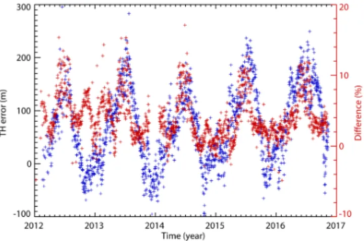
The ARRM has displayed the ability to track any drifts or sudden changes of 100 m (Sect. 3.3), and time series of TH error derived from the ARRM track very closely to the time
Figure 15. The time series of daily ARRM TH error (blue) and zonal mean ozone differences (%) between OMPS LP and Aura MLS (red) at 50◦N for the center slit. Note the similarity in time-dependent patterns for ozone differences and TH error derived from AARM method. The fact that these two completely independent methods show very similar patterns gives us additional confidence in ARRM.
to only a TH error or a MERRA error. It is important to note that MLS ozone profiles are reported as volume mixing ratio on a vertical pressure grid, while the LP algorithm retrieves ozone as number density on an altitude grid. Thus, in order to compare LP and MLS ozone retrievals, we had to convert ozone number densities to mixing ratios using MERRA tem-perature and GPH profiles. This conversion inevitably intro-duces MERRA GPH and temperature errors into the ozone comparisons. Therefore ozone differences between LP and MLS ozone retrievals depend not only on the LP TH error but also on errors in MERRA GPH as well as on errors in the retrieval algorithms and instrumental sampling (geophys-ical noise). Furthermore, analysis of LP and MLS ozone re-trievals indicates a large daily ozone variability at 3 hPa that ranges from 2 % in the tropics to 20 % at high latitudes with the seasonal maximum during austral winters (results are not shown here); this analysis provides a sense of the geophysical ozone variability that is present. In consideration of all of the above factors, we remain cautious in making definite conclu-sions regarding applying the ARRM results; further analysis and comparisons with independent ozone observations (like SAGE III) are needed to confirm the results.
5 Conclusions
Accurate altitude registration is key to the success of using limb-scattered radiances to retrieve atmospheric trace gases. We have described two scene-based techniques that together provide highly precise and accurate estimates of the tangent height. These altitude registration techniques are inexpensive and more comprehensive than external sources of altitude in-formation, such as star trackers mounted on the spacecraft. In
fact the star trackers on the SNPP spacecraft failed to detect the 1–1.5 km tangent height error that we derived by apply-ing the RSAS method (see Table 1). This error, if attributed to incorrect spacecraft pointing, means the nadir-viewing in-struments on SNPP were locating scenes 340 m too far south. Initial pointing errors of even greater magnitude have been observed (Wolfe et al., 2013).
The RSAS and ARRM techniques are complementary. We developed the latter because changes in tangent height errors are rather more important than static errors. Figure 9 suggests the relative accuracy of ARRM is sufficient to detect 100 m changes in pointing in the absence of GPH errors. The ac-curacy may not be so small when GPH errors are included, especially for time periods less than 1 year. Our expectation is that multi-year trends in GPH error are small, a position that is supported by the lack of observed OMPS TH trends after accounting for distinct pointing shifts. RSAS too can be used to monitor pointing changes, but its sensitivity to stratospheric aerosols means the results may be influenced by geophysical processes such as volcanic eruptions.
6 Data availability
The data set is available here: http://dx.doi.org/10.5067/ suomi-npp/omps-limb/l1-ev-grid/data12.
Acknowledgements. The authors gratefully acknowledge the
assis-tance of NASA’s limb processing team in providing the data used in this paper. We would also like to thank Dave Flittner, Ernest Nyaku, and Didier Rault, who helped with the development of and updates to the RT model. Finally, we would like to acknowledge the role Didier played in laying the groundwork for the OMPS limb retrieval algorithm.
Edited by: C. von Savigny
Reviewed by: two anonymous referees
References
Bourassa, A. E., Degenstein, D. A., Gattinger, R. L., and Llewellyn, E. J.: Stratospheric aerosol retrieval with optical spectrograph and infrared imaging system limb scatter measurements, J. Geo-phys. Res., 112, D10217, doi:10.1029/2006JD008079, 2007. Janz, S. J., Hilsenrath, E., Flittner, D. E., and Heath, D. F.:
Rayleigh scattering attitude sensor, Proc. SPIE, 146, 2831, doi:10.1117/12.257207, 1996.
Jaross, G., Bhartia, P. K., Chen, G., Kowitt, M., Haken, M., Chen, Z., Xu, P., Warner, J., and Kelly, T.: OMPS Limb Profiler instru-ment performance assessinstru-ment, J. Geophys. Res.-Atmos., 119, 4399–4412, doi:10.1002/2013JD020482, 2014.
Llewellyn, E. J., Lloyd, N. D., Degenstein, D. A., Gattinger, R. L., Petelina, S. V., Bourassa, A. E., Wiensz, J. T., Ivanov, E. V., McDade, I. C., Solheim, B. H., McConnell, J. C., Haley, C. S., von Savigny, C., Sioris, C. E., McLinden, C. A., Griffioen, E., Kaminski, J., Evans, W. F., Puckrin, E., Strong, K., Wehrle, V., Hum, R. H., Kendall, D. J. W., Matsushita, J., Murtagh, D. P., Brohede, S., Stegman, J., Witt, G., Barnes, G., Payne, W. F., Piche, L., Smith, K., Warshaw, G., Deslauniers, D. L., Marc-Hand, P., Richardson, E. H., King, R. A., Wevers, I., McCreath, W., Kyrölä, E., Oikarinen, L., Leppelmeier, G. W., Auvinen, H., Megie, G., Hauchecorne, A., Lefevre, F., de La Noe, J., Ricaud, P., Frisk, U., Sjoberg, F., von Scheele, F., and Nordh, L.: The OSIRIS instrument on the Odin spacecraft, Can. J. Phys., 82, 411–422, 2004.
Loughman, R., Flittner, D., Nyaku, E., and Bhartia, P. K.: Gauss– Seidel limb scattering (GSLS) radiative transfer model de-velopment in support of the Ozone Mapping and Profiler Suite (OMPS) limb profiler mission, Atmos. Chem. Phys., 15, 3007–3020, doi:10.5194/acp-15-3007-2015, 2015.
McGee, T. J., Whiteman, D., Ferrare, R., Butler, J. J., and Burris, J.: STROZ LITE: Stratospheric ozone lidar trailer experiment, Opt. Eng., 30, 31–39, 1991.
McPeters, R. D., Janz, S. J., Hilsenrath, E., Brown, T. L., Flittner, D. E., and Heath, D. F.: The retrieval of O3profiles from limb scatter measurements: Results from the Shuttle Ozone Limb Sounding Experiment, Geophys. Res. Lett., 27, 2597–2600, 2000. Rault, D. F.: Ozone profile retrieval from Stratospheric Aerosol and
Gas Experiment (SAGE III) limb scatter measurements, J. Geo-phy. Res., 110, D09309, doi:10.1029/2004JD004970, 2005.
Schwartz, M. J., Lambert, A., Manney, G. L., Read, W. G., Livesey, N. J., Froidevaux, L., Ao, C. O., Bernath, P. F., Boone, C. D., Cofield, R. E., Daffer, W. H., Drouin, B. J., Fetzer, E. J., Fuller, R. A., Jarnot, R. F., Jiang, J. H., Jiang, Y. B., Knosp, B. W., Krüger, K., Li, J.-L. F., Mlynczak, M. G., Pawson, S., Russell III, J. M., Santee, M. L., Snyder, W. V., Stek, P. C., Thurstans, R. P., Tomp-kins, A. M., Wagner, P. A., Walker, K. A., Waters, J. W., and Wu, D. L.: Validation of the Aura Microwave Limb Sounder temper-ature and geopotential height measurements, J. Geophys. Res, 113, D15S11, doi:10.1029/2007JD008783, 2008.
Sioris, C. E., Haley, C. S., McLinden, C. A., von Savigny, C., McDade, I. C., McConnell, J. C., Evans, W. F. J., Lloyd, N. D., Llewellyn, E. J., Chance, K. V., Kurosu, T. P., Murtagh, D., Frisk, U., Pfeilsticker, K., Bosch, H., Weidner, F., Strong, K., Stegman, J., and Megie, G.: Stratospheric profiles of nitro-gen dioxide observed by Optical Spectrograph and Infrared Im-ager System on the Odin satellite, J. Geophys. Res., 108, 4215, doi:10.1029/2002JD002672, 2003.
Taha, G., Jaross, G., Fussen, D., Vanhellemont, F., Kyrölä, E., and McPeters, R. D.: Ozone profile retrieval from GOMOS limb scattering measurements, J. Geophys. Res., 113, D23307, doi:10.1029/2007JD009409, 2008.
von Savigny, C., Kaiser, J. W., Bovensmann, H., Burrows, J. P., McDermid, I. S., and Leblanc, T.: Spatial and temporal charac-terization of SCIAMACHY limb pointing errors during the first three years of the mission, Atmos. Chem. Phys., 5, 2593–2602, doi:10.5194/acp-5-2593-2005, 2005.