Submitted11 June 2015 Accepted 6 March 2016 Published13 April 2016
Corresponding author Rami Puzis, puzis@bgu.ac.il
Academic editor Mohammad Reza Mousavi
Additional Information and Declarations can be found on page 18
DOI10.7717/peerj-cs.53
Copyright 2016 Dolev et al.
Distributed under
Creative Commons CC-BY 4.0
OPEN ACCESS
Efficient online detection of temporal
patterns
Shlomi Dolev1, Jonathan Goldfeld1, Rami Puzis2,3and Muni Venkateswarlu K.1
1Department of Computer Science, Ben-Gurion University, Beer-Sheva, Israel 2Telekom Innovation Laboratories, Ben-Gurion University, Beer Sheva, Israel
3Department of Information Systems Engineering, Ben-Gurion University, Beer-Sheva, Israel
ABSTRACT
Identifying a temporal pattern of events is a fundamental task of online (real-time) verification. We present efficient schemes for online monitoring of events for identifying desired/undesired patterns of events. The schemes use preprocessing to ensure that the number of comparisons during run-time is minimized. In particular, the first comparison following the time point when an execution sub-sequence cannot be further extended to satisfy the temporal requirements halts the process that monitors the sub-sequence.
SubjectsAlgorithms and Analysis of Algorithms, Theory and Formal Methods Keywords Pattern matching, Verification, Time series
INTRODUCTION
Many complex systems, both hardware and software, require sound verification of their operation, usually in the form of safety and liveness properties. One of the prominent formal verification methods used today is model checking, which models the system as a state-transition system, and performs an exhaustive search of its state-transition graph for possible runs where desired properties do not hold. In model checking, a precise description of the system to check is mandatory as, before actually running the system, all possible executions must be checked (Bauer, Leucker & Schallhart, 2011). One of the drawbacks of model checking is the state explosion problem (Rafe, Rahmani & Rashidi, 2013): explosion due to the need to explore an exponential number of states which grow with relation to the number of system variables. This yields a costly check. Another significant problem is in the modeling process itself. The verification is only as good as the model of the (actual hardware and software) implementation rather than the implementation itself. Online model checking is presented as a lightweight verification technique to overcome the state space explosion problem. However, the computational complexity of the proposed online model checking in time and space is less than that of (off-line) model checking, but greater than that of runtime verification (Zhao & Rammig, 2012).
to check for desired properties at runtime on the active execution path. System properties are written in a formal logic and then transformed into a runtime monitor (Colombo, Pace & Schneider, 2008). The transformations from design models to implementation are generally informal, therefore error-prone. Runtime verification validates transformations indirectly and provides a mechanism to handle exceptions of implementations that are not detected during development or testing (Dong et al., 2005).
We concentrated on a specific task of runtime verification; namely, the detection of temporal patterns. Rather than modeling the system and searching its entire state-transition graph, as is done in model checking, we devised an approach toward verification of time restrictions over sequences of events at system runtime. We used temporal constraint semantics to describe the specification.
Our contribution. We designed several algorithms which, given a description of the system as a set of possible events and a specification of safety properties as desired/undesired temporal patterns, monitor the system and detect when such patterns occur. We distinguished between several scenarios depending on the pattern profile: sporadic/continuous patterns, max-/max and min- constrained patterns.
First, we describe how to preprocess the input patterns in graph form to get their minimized representation by removing redundant constraints. Then, we describe an automaton which tracks pattern prefixes using tokens and detects pattern completion. This automaton tracks the system events efficiently. Once a token does not adhere to some temporal constraint, the token is discarded within one comparison; this is in addition an earliest possible notification on when a completed pattern is given.
Related work.Runtime verification is being pursued as a lightweight verification technique complementing verification techniques such as model checking and testing and establishes another trade-off point between these forces. One of the main distinguishing features of runtime verification is due to its nature of being performed at runtime, which opens up the possibility to act whenever incorrect software system behavior is detected (Leucker & Schallhart, 2009).
Runtime verification of asynchronous systems for ensuring safety and liveness specifications by monitoring events has been discussed in e.g., Dolev & Stomp (2003); Brukman & Dolev (2006);Brukman, Dolev & Kolodner (2008);Brukman & Dolev (2008). A parametric real-time monitoring system with multiple logical structures is proposed in Jin et al. (2012). Dynamic communicating automata with timers and events to describe properties of systems which need to be checked for different instances online are introduced inColombo, Pace & Schneider (2008). However, the implementation overhead is very high to implement this method.
A fundamental discussion of model checking appears in Clarke, Grumberg & Peled (1999), and a popular method to address the state explosion problem (Groote, Kouters & Osaiweran, 2012) of model checking is described inBurch et al. (1992), by representing the state transition graph using propositional logic formulae.Zhao & Rammig (2012)discusses a special form of online model checking method for runtime verification, which provide the model and implementation of the system to verify. A temporal logic is proposed in Baldan et al. (2006)to specify and verify properties on graph transformation systems. An approach of extending Computation Tree Logic(CTL) to include timing constraints appears inAlur, Courcoubetis & Dill (1993). InLaroussinie, Markey & Schnoebelen (2006), transitional durations are added to timed temporal formulae as an extension of Kripke Structures, and timed versions of CTL are considered. These frameworks however, do not address real-time verification.
Linear Temporal logic (LTL) has been used for runtime verification; however, it is best suited for design-time system verification. Also, the evaluation of LTL properties on finite traces proved to be an obstacle, as LTL is usually evaluated over infinite traces. The standard semantics of LTL on finite traces is unsatisfactory for the purpose at hand (Andreas, Martin & Christian, 2010).
Tools for real-time verification exist in the form of assertion checking, some of which follow the PSL IEEE standard, notablyColombo, Pace & Schneider (2008);Alur, Courcoubetis & Dill (1993);Brukman, Dolev & Kolodner (2008); further comparison of these tools is beyond the scope of this article. While these allow the specification of quite general properties and employ an automaton for detecting a single property, we focus on patterns with timing constraints and employ an automaton to detect all pattern instances.
Model programs have been rarely used for runtime verification (seeBlum & Wasserman, (1997) for example). As long as model programs are deterministic and contain no mandatory calls, they can be verified easily. But, for the model programs containing non-deterministic expressions or mandatory calls, we need tighter integration (Barnett & Schulte, 2003).
Organization.The formal setting is presented in the next section, along with detection of continuous temporal patterns. In ‘Sporadic Pattern Match,’ we study the less restricted definition of sporadic temporal patterns by analyzing the pattern’s temporal constraints, semantics, and devise a detection algorithm. Next, we briefly discuss an approach for estimating the probability of a partial pattern match completing a full pattern match in ‘Prediction and Alert of a Near Pattern Match.’ Finally, concluding remarks and future research scope appear in ‘Concluding Remarks.’
CONTINUOUS PATTERN MATCH
1a
jdenotes an event of typeaj.type.
teiandtei+1it holds thatti<ti+1. We assume that events in the system occur in discrete
time points (overZ).
Atemporal pattern TPis a tuple (A,C), whereA=(a1,a2,...,an) is a sequence of typed
(non-timed) events. Eachaihas a typeai.typefrom the event type set. Event types are not necessarily distinct:Cis a set oftemporal constraints, such that eachc∈Cis a tuple (ai,aj,w), where the time interval between the eventsaiandajis at mostw. We call such a constraint a max constraint; in ‘Adding minimum constraints’ we will address min constraints. Detection of continuous temporal patterns.We track a stream of timed events to identify temporal patterns that respect the constraints of TP. We consider the simple case of a continuous pattern. For every 1<i<n−1, we callai andai+1 consecutive events. A
continuous pattern matchis an execution sub-sequence where consecutive events happen successively. A (type-wise)1 executiona1,...,ai,b,ai+2,...,an whereb.type6=ai+1.typeis
not considered a match.
Directed graphs and tokens.A temporal pattern (A,C) is represented by apattern graph. The events inAdefine the graph nodes, and the constraints inCdefine edges. A constraint e=(ai,aj,w) wherei<jis a directed edge fromaitoaj with weightw. We denoteaiand aj bye.srcande.dst, respectively. If there is no constraint betweenaiandai+1for somei,
we define an edge (ai,ai+1,∞), where∞signifies that any finite time may pass between
aiandai+1. An edge between consecutive events is asimple edge, and any other edge is an
overpassing edge. A path using only simple edges is asimple path. (a1,a2,...,an) is defined as
thechronological orderof the pattern’s events. In particular,Gis a WDAG (Weighted DAG). A preprocessing phase of pattern constraints is explained in ‘Sporadic Pattern Match.’ Execution sub-sequences that partially match a pattern are represented by tokens. A token resides on an event, and carries with it a history of the time points at which it reached previous events. HandleEvent (Alg. 1) handles an event log received from the system in the form of a timed event (type,t), wheretypeis the event type andtis the time point at which it occurred. Iftknis a token currently residing on the graph, thentkn.evnt andtkn.hare the events on which the token resides, and the token’s history, respectively. The method getTime(a) oftkn.hreturns the time point at whichtknreacheda.
1 tkns := set of graph tokens; 2 ForEach tkn in tkns Do
3 b := successor of tkn.evnt;
4 If (b.type) != type Then discard tkn; 5 ForEach graph edge (a,b) Do
6 If (t - tkn.h.getTime(a) > w(a,b))
7 Then discard tkn;
8 add (b,t) to tkn.h;
9 tkn.evnt := b;
10 If (tkn.evnt is the last event) Then
11 report tkn;
12 discard tkn;
13 If (type matches the first event)
14 Then add a new token;
Figure 1 An example of token tracking for the event input stream: ((a,0),(b,12),(a,30),(c,37)).z2
be-comes obsolete whencoccurs.z1reaches the last eventcand completes a continuous pattern match.
In (line 1) we receive the set of graph tokens. We handle each such token (line 2). In (line 3) we obtain the successive event oftkn.evnt. If the event’s type does not matchtype (the logged event’s type), we discardtkn(line 4). We check if all edge constraints whose head isbare satisfied; If not, we discardtkn(lines 5–7). If the constraints are satisfied, we update the token’s history and movetknto the next event (lines 8–9). Iftknreaches the last pattern event, we report the pattern match and provide its history, and then discard tkn (lines 10–12). Finally, iftype matches the type of the first pattern event, we create a new token on the first event (lines 13–14).
An illustration of token tracking is shown inFig. 1.
SPORADIC PATTERN MATCH
Maximum constraintsAsporadic pattern matchis an execution sub-sequence where non-sequential system events may occur between consecutive pattern events. If the temporal pattern events area1,...,an, a
(type-wise) executiona1,...,ai,b,ai+1,...,anwhereb.type6=ai+1.typematches the pattern,
as long as the temporal constraints are satisfied. We designed an algorithm to detect sporadic pattern matches, so that a token is discarded at the very first constraint check once it becomes obsolete. We shall describe two phases of the pattern detection paradigm: a preprocessing phase and an on-line detection phase. The preprocessing phase will yield an equivalent temporal pattern in a more restrictive form. The online detection phase will utilize a many-state automaton to keep track of the system’s sub-sequence execution operation, which partially matching a pattern. The sub-sequences are represented by tokens that reside on the automaton’s states.
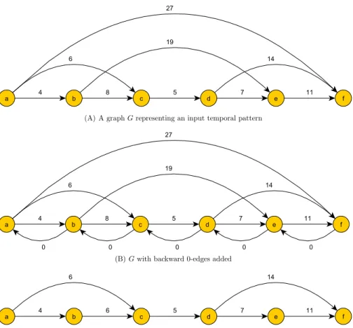
Preprocessing phase.In the preprocessing phase we reduce the pattern constraint set while maintaining the temporal constraint semantics. For every 1≤i<nwe add toGan edge (ai+1,ai,0), which we simply call a 0-edge. We compute the shortest path fromai toaj
Figure 2 Preprocessing phase of a temporal pattern graphG.
every simple edge to the weight of the shortest path between its ends. This update takes O(n2) comparisons. We denote the ensuing graph modulo the 0-edges asG′. An example of a graph before, during and after preprocessing can be seen inFigs. 2A,2Band2C. The role of 0 edges in finding the shortest path between the ends and updating edge weights is illustrated inFig. 3.
Histories and graph preorder.We call every single update ofGan update step. In the following discussion, the graphs are temporal patterns of nevents; the histories consist of these events. Ahistory is a tupleH=((a1,t1),...,(an,tn)), wheretj is the time-point
at whichaj occurred. We denotetj asH(aj). We denotetj−ti byH(ai,aj) or byH(e), wheree=(ai,aj,w) for somew. A historyH fitsa graphGif: for every (ai,ti) and (aj,tj) inH, if (ai,aj,t) is a weighted edge inG, thenH(ai,aj)6t. Alternatively, we sayH fits the underlying temporal patternTP.
We define a preorder≪(a reflexive and transitive relation) between graphs as follows: G1≪G2if for every historyH: (H fitsG1) implies that (H fitsG2). It is easy to show that
≪is indeed a preorder.≪naturally induces an equivalence relation≡on graphs:G1≡G2
ifG1≪G2andG2≪G1. In the following discussion, equivalence of graphs refers to the
Figure 3 Significance of 0 edges in reducing temporal constraint set.
Proposition 1 Let G and G′ be the graphs before and after the execution of preprocessing,
respectively. Then the following properties hold: Equivalence: G≡G′.
Minimality: G′ is the minimal graph that is equivalent to G. If any overpassing edge is removed from G′ or if the weight of some edge is reduced in G′, then it will no longer be
equivalent to G.
SeeAppendix S2for proof. This result is a special case of the results in ‘Adding minimum constraints’ and follows the result inDechter, Meiri & Pearl (1991).
On-line detection phase. We build an automatonTA whose states are the pattern of events. We may consider the graph as a representation of the automaton, with its events as different states. At any given time in the execution, an event may hold several tokens. A token represents a sub-sequence of the execution, partially matching the temporal pattern. The only transitions are from an eventai to the next eventai+1for every 1<i<n−1,
where the rule of the transition is that the token must satisfy the constraint of the simple edge (ai,ai+1). Additionally, a token must satisfy other constraints as explained in the
following schemes.
Deadline Scheme. Every tokentkn is associated with a minimum heaptkn.DL (for DeadLines) which is empty at first, and with a dynamic hash tabletkn.DLH. An element in the heap is a tuple (evnt,dl,ptr), wheredl is the deadline for the token to reach the event evnt. If the token does not reachevnt by the timedl, it becomes obsolete.ptr is a pointer to the twin element intkn.DLH. An element intkn.DLH is a tuple (evnt,ptr). The event evnt is the key, andptris a pointer to the twin elementtkn.DL. This duplication of data is necessary to ensure that no more than one instance of some event is in the heap.
1 tkns := tokens awaiting a type event; 2 ForEach tkn in tkns Do
3 m := tkn.DL.min;
4 If (m.dl < t) Then discard tkn; 5 b := successor of tkn.evnt;
6 If b is the last pattern event Then
7 report matched pattern;
8 discard tkn;
9 If (b has a token) Then discard b.tkn; 10 tkn’ := newToken(tkn,b,t)
11 If (m.evnt=b) Then remove m and m.ptr; 12 For (e in opEdges(b)) Do
13 c := e.dst;
14 If (c is in tkn’.DLH) Then
15 m0 := tkn’.DLH.get(c).ptr;
16 If (t+w(e) < m0.dl) Then
17 m0.dl := t+w(e);
18 heapify up m0;
19 Else
20 m0 := (c,t+w,null);
21 m1 := (c,m0);
22 m0.ptr := m1;
23 insert m0 into tkn.DL;
24 insert m1 into tkn.DLH;
25 If (type matches the first event) Then
26 add new token;
This keeps the space complexity of a token’s heap and hash table toO(n), instead of a possible2(n2) for2(n2) overpassing edges.tkn.evnt is the event on whichtknexists. We call this scheme thedeadline scheme.
If tknresides on eventaand the next chronological event in the patternboccurs at timet, we first checktknagainst the simple edge (a,b). If the constraint does not hold, tknis discarded fromTA. HandleEvent (Alg. 2) handles an event log (type,t). The method newToken(tkn,a,t) spawns a new tokenawhich inheritstkn’s history and adds the element (a,t) to the history of the new token.opEdges(a) returns the set of overpassing edges whose source isa.
In (line 1) we get the tokens awaiting atypeevent, in descending chronological order. We handle each subsequent token (line 2). In (line 3) we check the minimum elementm oftkn.DL. Ifm.dl<t,tknis discarded fromTAalong with its associated data structures, then we check the next token intkns(line 4). Iftknis valid and the next event is the last pattern event, we report a pattern match and discardtkn(lines 6–8). Otherwise, ifb, the next chronological event aftertkn.evnt,holds a token, then the old token is discarded (line 9). We spawn a new token tkn′on bthat inheritstkn.DLandtkn.DLH (line 10).
Ifm.evnt=b, we removemfromtkn′.DLandm.ptr fromtkn′.DLH (line 11), since this
deadline is no longer relevant. Furthermore, every overpassing edge that going frombmay contribute a deadline totkn′.DL: for every overpassing edgee=(b,c,w), we check if the
keycappears intkn′.DLH (line 14). If it appears as (c,ptr1), letptr1=m0=(c,dl,ptr0). If
t+w(e)<dl, we change the value ofdltot+w, and then movem0up the heap until the
heap property holds (lines 16–18). Ifdl≤t+w(e), we do nothing. Ifcdoes not appear in tkn′.DLH, we create twin elementsm
0=(c,t+w,ptr0) andm1=(c,ptr1), such thatptri
points tomi−1, and insert them intkn.DLandtkn.DLH, respectively (lines 19–24). Iftype
is the first pattern event type, we create a new token with an attached heap and hash table and add the appropriate deadlines (lines 25–26).
We handle the tokens by the events they reside, from late to early. The reason for this is as follows: say we have tokens on eventsaiandai+1, and the type of eventsai+1andai+2
istype, now atype event occurs. If we handle the token onaifirst, it will discard the token onai+1, though that token may spawn a token onai+2. Thus, we lose a possible pattern
match.
The reason we spawn a new tokentkn′ onai+1rather than movingtkntoai+1is that
ai+1may occur again while tknis still relevant. Thus spawning a new token tkn′′ with
different deadlines than those oftkn′. This algorithm ensures we detect the first instance of the temporal pattern during an execution. If we wish to detect all instances, we cannot discard a token (as in line 9), since it has a unique history, and may complete to a unique instance of the temporal pattern. If max{w(ai,ai+1)|1≤i≤n−1} =k, then there are at
mostO(kn) tokens at any point during the execution.
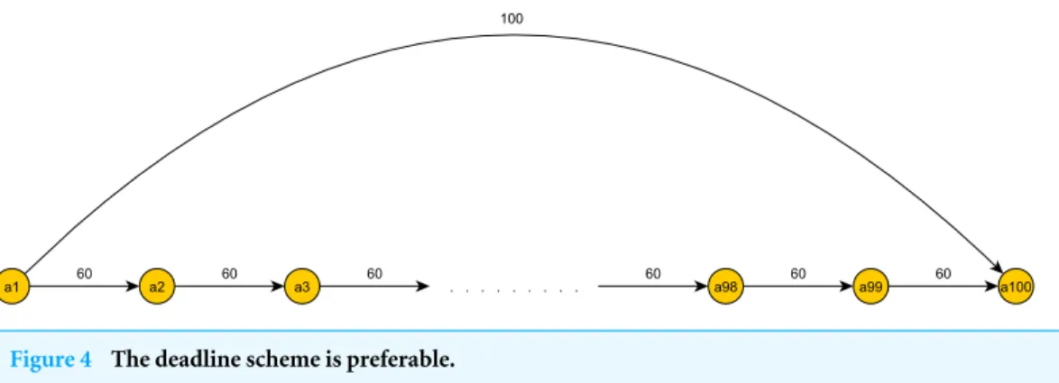
Figure 4 The deadline scheme is preferable.
Since we spawn tokens rather than moving them forward, per token here (and whenever we spawn tokens) refers to a given series of tokens that complete a pattern match. History scheme. Alternately, to the heap and hash table data structures, we may simply keep a history of the time points when a token reaches events; each time a token is spawned on an event, we compare the history with temporal constraints of overpassing edges whose destinations are the current event. We call this scheme thehistory scheme. Since there are nevents and each time we check back againstO(n) constraints, this adds up toO(n2) operations per token, which is better than the deadline scheme. We note that in both cases the token holds an associated data structure ofO(n) space.
There is still the matter of whether we detect an obsolete token as soon as it becomes so. For this to hold, we actually need to add overpassing edges to the graph after finding all shortest paths between pairs of nodes, with an edge’s weight set to the shortest path weight. The proof that this in fact ensures an earliest detection of an obsolete token is a special case ofProposition 2.
On the opposite extreme, we may consider the case presented below inFig. 4. Here, according to the history scheme, we add overpassing edges with weight 100 between all non-consecutive events. Thus, for a series of tokens spawning along the entire graph we will have2(n2) checks against constraints of overpassing edges, and it will use2(n2) space. On
the other hand, if we do not add edges, but maintain a heap of deadlines as in the deadline scheme, we will have only one deadline in the heap and one check against this deadline at each event a token reaches. Thus, the tokens will have only2(n) checks and will use only
2(n) space between them.
In fact, we used the history scheme in Alg. 1 to detect continuous pattern matches. We can also benefit from using the deadline scheme to detect such patterns, when there are few overpassing edges in the pattern graph.
What is the differential line between using one scheme and not the other? A straightforward calculation follows. Let k be the number of overpassing edges in the graph. Then in the deadline scheme, a token will haveO(k·log(n)+n) operations. In the history scheme we may have up toO(n2) overpassing edges as in the example inFig. 4. Thus a starting point for finding the differential line isk=O(n2/log(n)). Furthermore,
wherek=1. In this case, we have a better number of operations and space complexity for the deadline scheme, namelyO(n) andO(1), respectively.
Adding minimum constraints
We now broaden our scope by allowing input patterns with both maximum and minimum constraints. We highlight the differences in definitions and notations that ensue. Here a temporal pattern input is a triplet TP=(A,CMax,CMin).Ais the sequence of events: A=(a1,a2,...,an).CMaxis a set of maximum temporal constraints (max constraints) on
A. An element ofCMax is (ai,aj,t), wheret is the maximum time allowed betweeneiand ej.CMinis a set of minimum temporal constraints (min constraints) onA. An element of CMinis (ai,aj,t), wheret is the minimum time allowed betweeneiandej.
We note that a temporal constraint may be 0 or∞. Furthermore, one may change the model slightly by allowing only strictly positive time intervals for the min constraints, i.e., each constraint is of value at least 1. This simply amounts to adding the constraints (ai,ai+1,1) toCMinfor every 1<i<n−1. In general, we may define in our model (or
get a restriction as input) that all constraints must be in the time window (m,M) for some m,M∈Nwherem6M. This amounts to adding the constraints (ai,ai+1,m) toCMinand
(ai,ai+1,M) toCMaxfor every 1<i<n−1.
Preprocessing phase. The definition of a history fitting a temporal pattern is similar to ‘Maximum constraints,’ only the history should adhere to both min and max constraints. We describe the preprocessing process. We build a weighted, directed graph G=(A,E), where nodes are the events inA, and edges areE= {(ai,aj,t)|(ai,aj,t)∈
CMax}S{(aj,ai,−t)|(ai,aj,t)∈CMin}. Also, there’s an edge (ai,ai+1,∞) or (ai+1,ai,0)
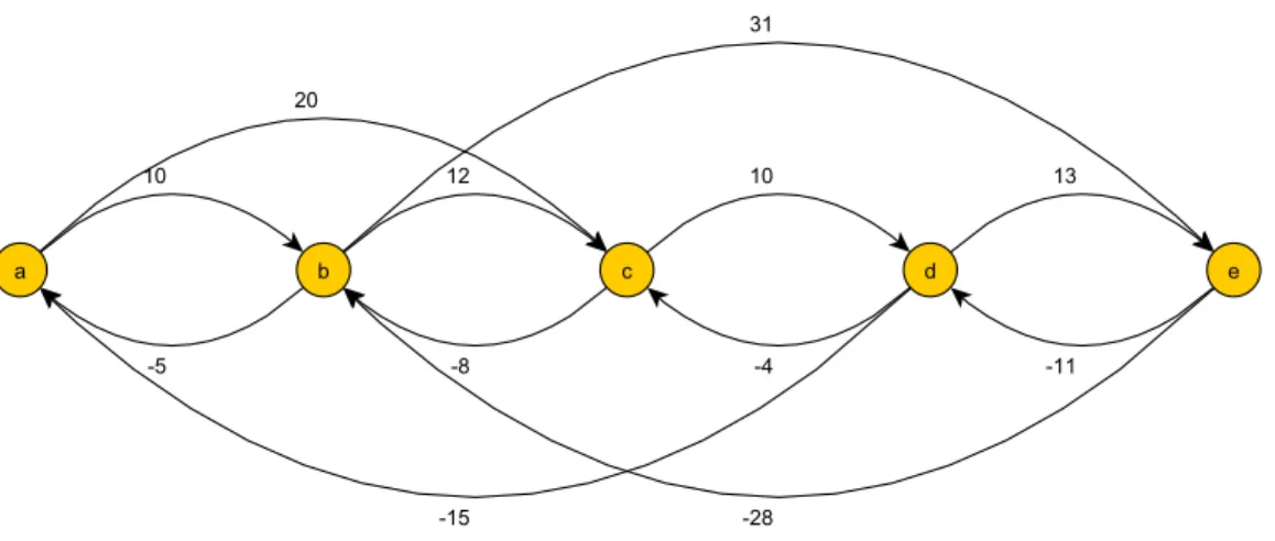
for consecutive events without a constraint inCMaxorCMin, respectively. The purpose of this construction is again to utilize the Floyd–Warshall algorithm for finding all shortest paths. Here we will have a ‘‘window of opportunity’’ for every pair of eventsai andaj that will indicate the exact time frame in which a token residing on ai must reachaj to hold by the constraints. We call this window a time window forai andaj. We run the Floyd–Warshall algorithm to find the shortest paths between all pairs of nodes inG. Our purpose is to contract the time windows as much as possible for all pairs of events. An example graph is depicted inFig. 5.
Time windows. Next we define the time windows. Let min(a,b) be the weight of the shortest (a,b)-path. For all 1<i<j<n:tw(ai,aj)=(−min(aj,ai),min(ai,aj)). We denote the set of all time windows ofTPasTW(TP).aiandajare called thesourceanddestination oftw(ai,aj) respectively, and are denoted bysrc(tw) anddst(tw), respectively. The first index of a time windowtw is called thelower bound oftw, denoted astw. The second index is called the upper bound, denoted as tw. A time window between consecutive events ai andai+1 is called asimple time window. Iftwi(ai,bi) andtwj(aj,bj) are time
windows such that (aj<∼ai∨aj=ai)∧(bi<∼bj∨bi=bj), we say thattwi issubsumed
bytwj. If H is a history andtw is a time window between eventsaandb, thenH(tw) denotes H(a,b). Formally, we defineCMax′= {(ai,aj,min(ai,aj)|ai,aj∈A,ai
∼
<aj)},
CMin′= {(ai,aj,−min(aj,ai)|ai,aj∈A,ai ∼
Figure 5 A graph for max and min constraints temporal pattern.The shortest (b,d)-path, ((b,e)(e,d)), has weight 20. The shortest (d,b)-path, ((d,e)(e,b)), has weight−15. Following the preprocessing phase, we get thattw(b,d)=(15,20).
thatTP≡TP′.TP′is in fact the temporal constraints closure ofTP. These updates maintain temporal constraint semantics (Proposition 2).
Another case to consider is whether the temporal pattern is consistent; whether there is a history that fits the pattern. If, for example, we have the constraints: (a,b,10),(b,c,7)∈CMax, and (a,c,24)∈CMin, there is a contradiction in the temporal semantics of the temporal pattern, and no history can fit the pattern. However, not all contradictions may manifest in so obvious a fashion. Fortunately, this happens exactly when there is a negative cycle (a cycle with negative weight) inG, something we can detect with a slight modification of the Floyd–Warshall algorithm.
Proposition 2 Let TP and TP′ be the temporal patterns before and after the executing
preprocessing, respectively. Then the following properties hold: Equivalence: TP≡TP′.
No-Negative: There exists a history H that fits TP⇐⇒there is no negative cycle in G. Minimality: Assuming there is no negative cycle in G, then: TP′ is the minimal graph that
is equivalent to TP, i.e., any further contraction of any time window in TP′ will result in a temporal pattern TP′′ that is not equivalent to TP′.
SeeAppendix S2for proof. A different form of the proof has appeared in the framework of Temporal Constraint Networks (Dechter, Meiri & Pearl, 1991), and in particular the no-negative result has appeared inLeiserson & Saxe (1983);Liao & Wong (1983).
On-line detection phase.First, we observe that, unlike Alg. 2 (lines 8–9), an older token fromai+1cannot be discarded when a new token is spawned, as the older token may
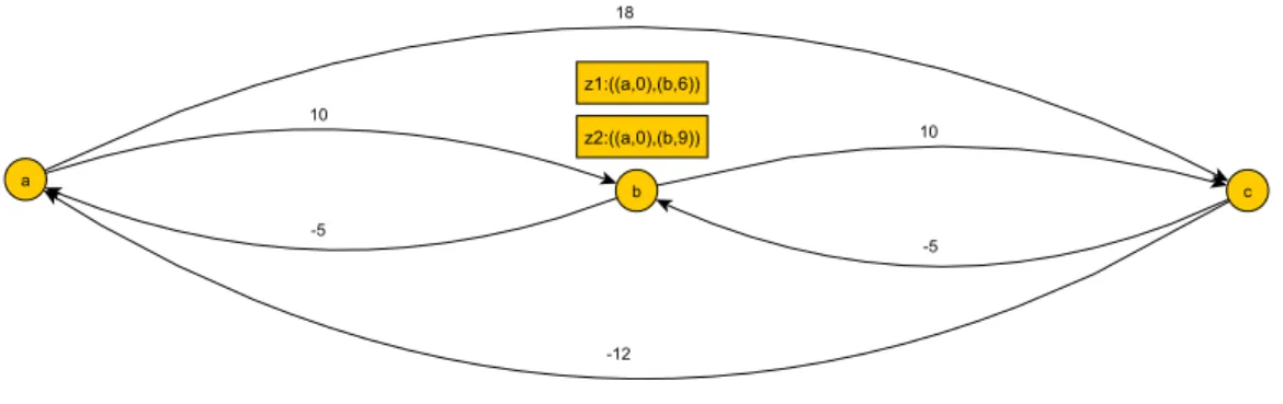
complete a pattern match while the new one does not, and vice versa. SeeFig. 6for an illustrating example.
Figure 6 An example of a temporal pattern for min and max constraints after preprocessing.Given the history ((a,0),(b,6),(b,9)) we have two tokens onbwith different histories. If (c,13) occursz1will
ad-vance whilez2will not, and if (c,17) occursz2will advance whilez1will not.
complete a pattern match. Hence, if we use the history scheme in keeping a history for each token, whenever the token reaches an event we can check back against constraints with earlier events. Such a simple scheme ensures the earliest detection of an obsolete token. This amounts to keeping anO(n) space history per token, and performingO(n2) total checks per token that traverses the entire graph. Since we have2(n2) overpassing edges,
it seems at a first glance that the deadline scheme is not efficient, since we haven2·log(n) operations andO(n) space per token, as in ‘Maximum constraints.’
However, if we examine the temporal pattern depicted inFig. 4where all min constraints are 0, we see that we need to save only one deadline for a token and performO(n) checks in total, which is better than the history scheme. Defining all time windows is unnecessary and is in fact a hindrance, since the time windows do not add information; the given graph already follows the temporal constraints closure of the temporal pattern. Using the history scheme here is inefficient: Roughly speaking, as the graph gets richer with more max and min constraints, the history scheme becomes more plausible, since the preprocessing phase will yield much more information in the form of contracted time windows.
PREDICTION AND ALERT OF A NEAR PATTERN MATCH
We conduct an analysis to estimate the chances of a token representing a partial pattern to complete a pattern match, henceforth the token’scompletion probability. We assume events of all types have equal probabilitypof occurring at any time point.Probabilistic settings.Our computation advances in parallel to the chronological order of the pattern events. For each event we reach, we examine the distinct possibilities of the next event (or rather, its type) occurring in the desired time frame—in the necessary time window. We start with a basic example to illustrate the computation process.
Assume we have a two event temporal pattern with eventsa0,a1and a time window
tw(a0,a1)=(m,M). Leta0occur at time 0, so that we have a token ona0representing
a partial patternP0. We haveM−m+1 distinct possibilities forP0to complete. The
probability ofa1.type not occurring at timesm,m+1,...,m+j−1 and occurring at time
Now, assume we have a temporal patternTPwithn+1 events,a0,...,an. We start with
a simple example where the pattern graph has only simple edges (for both max and min constraints). In such a case, if the probability of a token advancing froma0toa1isp(1)and
the probability of it later advancing froma1toa2isp(2), then the probability of the token
getting froma0toa2isp(1)·p(2). The overlying fact that governs this result is the lack of
dependencies between the two advancement steps, which is in turn due to the lack of an overpassing edge that encompasses the interval of events froma0toa2. To generalize, if
the probability of a token advancing fromai−1toaiisp(i), then we get in this case that the
completion probability of a token at the beginning of the temporal pattern isQni=1p(i). If
tw(ai−1,ai)=(mi,Mi), 0≤i≤n−1, then we get that the precise completion probability is
Qn i=1
PMi−mi
j=0 (1−p)jp=pn
Qn
i=1[1−(1−p)Mi−mi+1].
Now, assume we have some general pattern where there may be overpassing edges in the pattern graph. Say we have a token residing on ai, with a partially fitting history H= {(ar,tr)}ir=0:Hmay (and probably does) limit the times at which the token may reach subsequent events. In other words, it further contracts the time windows ofTP for this token. Next, we examine how a token’s history impacts the subsequent time windows and the computation of the token’s completion probability.
History restrictions and induced pattern graphs
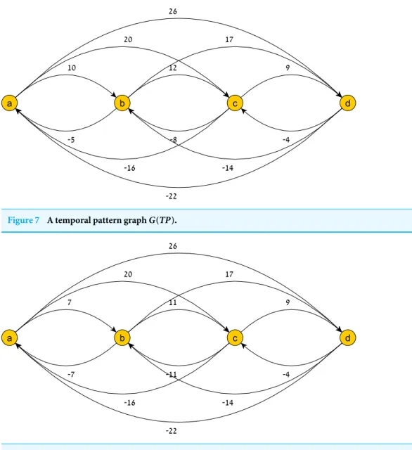
First we provide some notational groundwork. LetTP=(A,CMax,CMin) and letC(H)= {(ai,ai+1,H(ai,ai+1))}ir=−01. We define TP|H=(A,CMax ∪ C(H),CMin ∪ C(H)). In other words, C(H) is the set of constraints defined by the historyH, andTP|H is the restriction ofTP to temporal patterns that admit only histories that containH as their fitting histories. We defineG(TP) as the graph (A,E), where the nodes inAare the events of TP, and the edges areE= {−tw(aj,ai)}1≤i≤j≤nS{tw(ai,aj)}1≤i≤j≤n. In other words,
G(TP) is the pattern graph induced byTP∗ (the closure ofTP, see ‘Adding minimum constraints’). For a pattern graphG=(A,E) and a partially fitting historyH, we define EMax = {(ai,ai+1,H(ai,ai+1)}1≤i≤|H|−1,EMin= {(ai+1,ai,−H(ai,ai+1)}1≤i≤|H|−1, and
G|H=(A,E∪EMax∪EMin).
Illustrations of a temporal pattern graph and its restriction to a history are shown in Figs. 7and8, respectively.
Note that the new edges defined byH replace the old ones (they are more restrictive). Simply put, the induced graph represents a new temporal pattern that includesH in its account of temporal constraints. If the time that passed between eventsaiandai+1inH is
t, and if we wish to define a new temporal pattern that admits only histories containingH as a subset, we should add the (both max and min) temporal constraint (ai,ai+1,t).
In order to compute the time window defined byHbetween eventsarandar+1, we need
to find the shortest (ar,ar+1)-pathand (ar+1,ar)-pathinG|H. If the probability of this distinct history isp(H)=pj1pj2...pji, and the time window defined byH for reachingai+1
is of sizek′, then we havek′+1 branchings of possible continuations ofH and appropriate
probability factors added to p(H). Namely, the branchings and their probabilities are pj1pj2...pjipjl , 0≤j≤k
′. IfPl
i=1ji=j, we denotepj1pj2...pjl=
Ql
i=1(1−p)jip=pl·(1−p)j
Figure 7 A temporal pattern graphG(TP).
Figure 8 A history-restricted pattern graph.The graphG(TP|H) ofTP’s restriction to the historyH=
((a,0),(b,7),(c,18)).
Thus, if we have a token residing on the first event of a temporal pattern and we wish to compute its completion probability, we should sum up all the possible history branches and their probabilities. We can envision this branching computational process as a tree of histories, where each (full and fitting) history will be a path from the root of the tree to a leaf, representing a distinct probability of a token completing to a pattern match. We therefore sum all the possibilities (defined by distinct histories) of a token completing to a pattern match, and add-up to get the desired completion probability of the token.
We recall the definition of a temporal pattern’s girth:g(TP)=max{tw−tw+1|tw∈
TW(TP)∧twis a simple time window}. Thus, for a temporal patternTP withnevents, andg(TP)=k, the calculation of the completion probability for a token on the first event will takeO(d·kn) time, wheredis the time it takes to compute the shortest (ai,ai+1)-path
Figure 9 An illustration of the shortest paths induced by a history.An illustration of the shortest paths induced by H. 1. illustrates the shortest (ar,ar+1)-path and 2. illustrates the shortest (ar+1,ar)-path.
A more tractable problem is predicting the completion probability of a token residing on an eventai, wheren−i is bounded by some smalll. We then get anO(d·kl) time complexity for calculating a token’s completion probability. Hence, for a small enoughl, sayl=O(logkn), we get a time complexity ofO(d·n). To generalize, ifl=O(polylogk(n)), we get a time complexity ofO(d·poly(n)).
Recomputing the shortest paths between consecutive events
Finding the size of the next time window at each level of the probability tree can be done in linear time due to the following fact: The shortest (ar,ar+1)-pathand (ar+1,ar)-pathin
G(TP|H) for some 1≤r≤n−1 and a partially fitting historyH=((ai,ti))ri=1must take
the form of using a series of edges out of the new simple edges induced byH and a single overpassing edge from the beginning of this series toar+1.Fig. 9is an illustration of these
paths.
The following lemma formalizes this fact.
Lemma 3. Let TP be a temporal pattern, and let H=((ai,ti))ri=1for some1≤r≤n−1be some partially fitting history of TP. Then the following hold:
•The shortest (ar,ar+1)- path in G(TP|H)is((ar,ar−1,H(ar−1,ar)),(ar−1,ar−2,H(ar−2,
ar−1)),...,(aj+1,aj,H(aj,aj+1)),(aj,ar+1,w))for some 1≤j ≤r, where (aj,ar+1,w)is a
maximum constraint in TP∗.
•The shortest(ar+1,ar)- path in G(TP|H)is((ar+1,aj,w),(aj,aj+1,H(aj,aj+1)),(aj+1,aj+2,
H(aj+1,aj+2)),...,(ar−1,ar,H(ar−1,ar))) for some 1≤j ≤r, where (ar+1,aj,−w)is a
minimum constraint in TP∗.
SeeAppendix S2for proof.
l takesO(n·kl) time complexity, wherek=g(TP). Ifl=O(logkn) we get anO(n2) time complexity. Generally, ifl=O(polylogk(n)), we get a time complexity ofO(poly(n)).
Also note that iflandk are bounded, we get a time complexity that is linear inn.
Aggregating completion probabilities
We summarize how the completion probability can be computed using a polynomial-size data structure to reduce the number of arithmetic computations. Due to space considerations, the complete algorithm is not shown.
We recall our discussion of the tree of histories which we call aprobability tree. Each history is a path from the root down to a leaf. The root represents the token’s relative zero-time, i.e., the time from which we wish to compute the token’s completion probability. An edgePxi to a node in the tree represents a time point with a shift ofxi time points relative to the beginning of the current time window, contributing a factor of pxi to the current
probability path. The set of a node’s children in the tree represents the different possibilities of the current history’s continuation. In other words, suppose the current probability path counts the factors px1px2...pxd =pd(1−p)Pdi=1xi. If we compute x=Pd
i=1xi, we have
Qd
i=1pxi=p ∗
d,x. Suppose the next time window is of sizek′, then the edges to the current node’s children areP0,P1,...,Pk′, and continuing along an edgePx
d+1,0≤xd+1≤k
′adds
the factorpxd+1 to the above multiple, yieldingp
d+1(1−p)Pdi=+11xi=p∗
d+1,x+xd+1.
What we get here is in fact multiple paths that lead to the same probability. LetT be a probability tree, and letPaths(T) be the set of rooted paths inT ending in a leaf. Then the token’s completion probability equalsPP∈Paths(T)p∗
ρ(P), whereρ(P) denotes the value of
the last node inP.
Furthermore, ifTP is the temporal pattern andk=g(TP), then the maximal value of a leaf isk·l, since every node along a path from the root to the leaf contributes at most a factor ofp∗
k. Hence, there are at mostk·l+1 leaves and we can use an array of sizek·l+1 to count the instances of everyp∗
j, 0≤j≤k·l.
CONCLUDING REMARKS
In this work we introduced a novel framework for monitoring real-time systems for undesired behavior, based upon specifications given as temporal patterns. The system specifications are described using temporal constraint semantics. Instead of modeling and searching the system for its entire state-transition graph, as done in model checking, we proposed an approach to verify sequence of system events at runtime with time restrictions over the events. We devised a process for finding the closure of the temporal constraints semantics to reduce the pattern constraint set while maintaining the temporal constraint semantics, and provided different schemes for on-line detection of temporal patterns. The earliest possible notification on completed patterns helps the system to reduce number of comparisons during systems’ pattern match execution. An analysis is provided to predict and estimate the chances of a token representing a partial pattern to complete a pattern match.
Specifications of properties for on-line verification may be more complex. Hence, another line of research may broaden the input scope of temporal patterns as boolean formulae, where constraints are variables and histories are assignments. We sayH fits a temporal pattern formula if it evaluates toTrueunderH. We define the languageTP-SAT as all temporal pattern formulae TP, such that there exists a historyH that fitsTP. TP-SAT∈NP, and it is easy to show by a reduction fromSAT thatTP-SAT is NP-Hard. However, some families of formulae may be tractable. The DNF formulae, for example, may be seen as a collection of regular temporal patterns with the same sequence of events (albeit different temporal constraints), and handled accordingly.
Furthermore, the probabilistic settings may be expanded to include different probabilities for different event types, though the computations would be similar. Setting non-uniform distributions on the other hand may necessitate a different approach.
ACKNOWLEDGEMENTS
We thank the editor and all the reviewers for their valuable suggestions and ideas to improve the standards of the paper.
ADDITIONAL INFORMATION AND DECLARATIONS
Funding
This work is partially supported by Deutsche Telekom, the Rita Altura Trust Chair in Computer Sciences, the Lynne and William Frankel Center for Computer Sciences, the Israel Science Foundation (grant number 428/11), the Cabarnit Cyber Security MAGNET Consortium, a grant from the Institute for Future Defense Technologies Research named for the Medvedi of the Technion, the Israeli Internet Association, and the Israeli Defense Secretary (MAFAT). The funders had no role in study design, data collection and analysis, decision to publish, or preparation of the manuscript.
Grant Disclosures
The following grant information was disclosed by the authors: Deutsche Telekom.
Rita Altura Trust Chair in Computer Sciences.
Lynne and William Frankel Center for Computer Sciences. Israel Science Foundation: 428/11.
Cabarnit Cyber Security MAGNET Consortium. Institute for Future Defense Technologies Research. Israeli Internet Association.
Israeli Defense Secretary (MAFAT).
Competing Interests
Author Contributions
• Shlomi Dolev and Rami Puzis contributed reagents/materials/analysis tools, wrote the paper, reviewed drafts of the paper, proofs and algorithm analysis.
• Jonathan Goldfeld contributed reagents/materials/analysis tools, wrote the paper, prepared figures and/or tables, performed the computation work, reviewed drafts of the paper, proofs and algorithm analysis.
• Muni Venkateswarlu K. wrote the paper, prepared figures and/or tables, reviewed drafts of the paper.
Data Availability
The following information was supplied regarding data availability: The research in this article did not generate any raw data.
Supplemental Information
Supplemental information for this article can be found online athttp://dx.doi.org/10.7717/ peerj-cs.53#supplemental-information.
REFERENCES
Alur R, Courcoubetis C, Dill D. 1993.Model-checking in dense real-time.Information and Computation104(1):2–34DOI 10.1006/inco.1993.1024.
Andreas B, Martin L, Christian S. 2010.Comparing LTL semantics for runtime verifica-tion.Journal of Logic and Computation20(3):651–674DOI 10.1093/logcom/exn075. Baldan P, Corradini A, Konig B, Lafuente AL. 2006. A temporal graph logic for
verification of graph transformation systems. In:18th international workshop on algebraic development techniques, 1–20.
Barnett M, Schulte W. 2003.Contracts, components, and their runtime verifica-tion on the .NET platform.Journal of Systems and Software65(3):199–208 DOI 10.1016/S0164-1212(02)00041-9.
Bauer A, Leucker M, Schallhart C. 2011.Runtime verification for LTL and TLTL.ACM Transactions on Software Engineering and Methodology20(4): Article 14.
Blum M, Wasserman H. 1997.Software reliability via run-time result-checking.Journal of the ACM 44(6):826–849DOI 10.1145/268999.269003.
Brukman O, Dolev S. 2006. Recovery oriented programming. In:Proceedings of the 8th international symposium on stabilization, safety, and security of distributed systems (SSS 2006), LNCS, vol. 4280. New York: Springer, 152–168.
Brukman O, Dolev S. 2008. Self-* programming run-time parallel control search for reflection-box. In:Proceedings of the 6th NASA langley formal methods workshop. A poster in the Second IEEE international conference on self-adaptive and self-organizing systems, (SASO) 2008. Piscataway: IEEE.
Burch JR, Clarke EM, McMillan KL, Dill DL, Hwang LJ. 1992.Symbolic model checking: 1020states and beyond.Information and Computation98(2):142–170 DOI 10.1016/0890-5401(92)90017-A.
Clarke EM, Grumberg O, Peled DA. 1999.Model checking. Cambridge: MIT Press. Colombo C, Pace GJ, Schneider G. 2008.Dynamic event-based runtime monitoring
of real-time and contextual properties. In:13th international workshop on formal methods for industrial critical systems, 135–149.
Crochemore M. 1988. String matching with constraints. In:Proc. MFCS’88 symp. Lecture notes in computer science, Vol. 324. Berlin: Springer, 44–58.
Dechter R, Meiri I, Pearl J. 1991.Temporal constraint networks.Artificial Intelligence 49:61–95DOI 10.1016/0004-3702(91)90006-6.
Dolev S, Stomp F. 2003.Safety assurance via on-line monitoring.Distributed Computing 16(4):269–277DOI 10.1007/s00446-003-0089-5.
Dong Z, Fu Y, Fu Y, He X. 2005.Automated runtime validation of software architecture design. In:Second international conference distributed computing and internet technology—ICDCIT 2005, 446–457.
Groote JF, Kouters TWDM, Osaiweran A. 2012. Specification guidelines to avoid the state space explosion problem. In:Processdings of the fundamentals of software engineering. LNCS, vol. 7141. New York: Springer, 112–127.
Jin D, Meredith PO, Lee C, Ros u G. 2012.JavaMOP: efficient parametric runtime monitoring framework. In:Proceedings of the 34th international conference on software engineering, 1427–1430.
Laroussinie F, Markey N, Schnoebelen P. 2006.Efficient timed model checking for discrete-time systems.Theoretical Computer Science353(1):249–271
DOI 10.1016/j.tcs.2005.11.020.
Leiserson CE, Saxe JB. 1983. A mixed-integer linear programming problem which is efficiently solvable. 204–213.
Leucker M, Schallhart C. 2009.A brief account of runtime verification.The Journal of Logic and Algebraic Programming 78(5):293–303DOI 10.1016/j.jlap.2008.08.004. Liao YZ, Wong CK. 1983.An algorithm to Compact a VLSI symbolic layout with mixed
constraints.IEEE Transactions on Computer-Aided Design of Integrated Circuits and Systems2(2):62–69DOI 10.1109/TCAD.1983.1270022.
Luo L. Software testing techniques: technology maturation and research strategies. In: International Institute for Software Research. Pittsburge: Carnegie Mellon University. Rafe V, Rahmani M, Rashidi K. 2013.A survey on coping with the state space explosion
problem in model checking.International Research Journal of Applied and Basic Sciences4(6):1379–1384.
Zeigler B, Kim TG, Praehofer H. 2000.Theory of modeling and simulation. Second edition. New York: Academic Press.