Recognition
Weifeng Liu1, Yang Li1, Xu Lin2,3, Dacheng Tao4*, Yanjiang Wang1
1College of Information and Control Engineering, China University of Petroleum (East China), Qingdao, Shandong, China,2Shenzhen Institutes of Advanced Technology, Chinese Academy of Sciences, Shenzhen, Guangdong, China,3The Chinese University of Hong Kong, Hong Kong, China,4Centre for Quantum Computation and Intelligent Systems, and Faculty of Engineering and Information Technology, University of Technology, Sydney, Ultimo, New South Wales, Australia
Abstract
Co-training is a major multi-view learning paradigm that alternately trains two classifiers on two distinct views and maximizes the mutual agreement on the two-view unlabeled data. Traditional co-training algorithms usually train a learner on each view separately and then force the learners to be consistent across views. Although many co-trainings have been developed, it is quite possible that a learner will receive erroneous labels for unlabeled data when the other learner has only mediocre accuracy. This usually happens in the first rounds of co-training, when there are only a few labeled examples. As a result, co-training algorithms often have unstable performance. In this paper, Hessian-regularized co-training is proposed to overcome these limitations. Specifically, each Hessian is obtained from a particular view of examples; Hessian regularization is then integrated into the learner training process of each view by penalizing the regression function along the potential manifold. Hessian can properly exploit the local structure of the underlying data manifold. Hessian regularization significantly boosts the generalizability of a classifier, especially when there are a small number of labeled examples and a large number of unlabeled examples. To evaluate the proposed method, extensive experiments were conducted on the unstructured social activity attribute (USAA) dataset for social activity recognition. Our results demonstrate that the proposed method outperforms baseline methods, including the traditional co-training and LapCo algorithms.
Citation:Liu W, Li Y, Lin X, Tao D, Wang Y (2014) Hessian-Regularized Co-Training for Social Activity Recognition. PLoS ONE 9(9): e108474. doi:10.1371/journal. pone.0108474
Editor:Kewei Chen, Banner Alzheimer’s Institute, United States of America
ReceivedMay 30, 2014;AcceptedAugust 28, 2014;PublishedSeptember 26, 2014
Copyright:ß2014 Liu et al. This is an open-access article distributed under the terms of the Creative Commons Attribution License, which permits unrestricted use, distribution, and reproduction in any medium, provided the original author and source are credited.
Data Availability:The authors confirm that all data underlying the findings are fully available without restriction. All relevant data are within the paper.
Funding:Weifeng Liu is supported by the National Natural Science Foundation of China (61301242), Shandong Provincial Natural Science Foundation, China (ZR2011FQ016), and the Fundamental Research Funds for the Central Universities, China University of Petroleum (East China) (13CX02096A). Dacheng Tao is supported by Australian Research Council Projects DP-120103730, FT-130101457, and LP-140100569. Yanjiang Wang is supported by the National Natural Science Foundation of China (61271407). The funders had no role in study design, data collection and analysis, decision to publish, or preparation of the manuscript.
Competing Interests:The authors have declared that no competing interests exist.
* Email: [email protected]
Introduction
The rapid development of Internet technology and computer hardware has resulted in an exponential increase in the quantity of data uploaded and shared on media platforms [1] [2]. Processing these data presents a major challenge to machine learning, especially since most of the data are unlabeled and are described by multiple representations in different computer vision applica-tions [3] [4]. One of the earliest multi-view learning schemes was co-training, in which two classifiers are alternately trained on two distinct views in order to maximize the mutual agreement between the two views of unlabeled data [5]. In general, the co-training algorithms train a learner on each view separately and then force the learners to be consistent across views.
A number of co-training approaches have been proposed in many applications [6] [7] [8] [9] since the original implementation [10] [11] and can be divided into four groups: (1) co-EM [12] [13]; (2) regression [14] [15]; (3) regularization [16]; and (4) co-clustering. The co-EM algorithm combines co-training with the probabilistic EM approach by using naive Bayes as the underlying learner [12]. Brefeld and Scheffer [13] subsequently developed a EM version of support vector machines (SVMs). The co-regression algorithm can also be used to extend co-training to
regression problems; for example, Zhou and Li [14] employed two k-nearest neighbor regressors with different distance metrics to develop a co-training style semi-supervised regression algorithm, and Brefeld et al. [15] investigated a semi-supervised least squares regression algorithm based on the learning schema. The co-regularization algorithm formulates co-training as a joint com-plexity regularization between the two hypothesis spaces, each of which contains a predictor approximating the target function [16]. The clustering algorithms [17] [18] [19] apply the idea of co-training to unsupervised learning settings with the assumption that a point will be assigned to the same cluster in each view by the true underlying clustering.
Although many co-training variants have been developed, most co-training-style methods aim to obtain satisfactory performance in multi-view learning by minimizing the disagreement between two classifiers. However, it is likely that a learner will receive erroneous labels on unlabeled data when the other learner has only mediocre accuracy. This usually happens in the first rounds of co-training, when there are only a few label examples.
particular view of examples, which is then used to penalize the classifier along the potential manifold. Comparing other manifold regularizations e.g. Laplacian regularization, Hessian has a richer nullspace and steers the learned function that varies linearly along the underlying manifold. Thus Hessians can properly exploit the local distribution geometry of the underlying data manifold [20] [21], and therefore Hessian regularization can significantly boost the generalizability of a classifier, especially when only a small number of labeled examples exist with a large number of unlabeled examples.
To evaluate the proposed Hessian regularized co-training, we conduct extensive experimentation on the unstructured social activity attribute (USAA) dataset [22] [23] for social activity recognition [24] [25] [26] [27]. The USAA dataset contains eight different semantic class videos, which are home videos of social occasions, including birthday parties, graduation parties, music performances, non-music performances, parades, wedding cere-monies, wedding dances, and wedding receptions. We compare the proposed Hessian regularized co-training (HesCo) with traditional co-training and Laplacian regularized co-training Table 1.List of important notations.
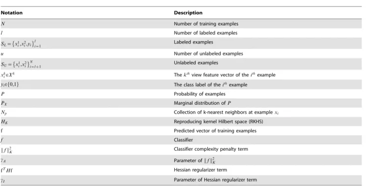
Notation Description
N Number of training examples
l Number of labeled examples
SL~ x1
i,x2i,yi l
i~1 Labeled examples
u Number of unlabeled examples
SU~ x1i,x2i N
i~lz1 Unlabeled examples
xk
i[Xk Thekthview feature vector of theithexample
yi[f0,1g The class label of theithexample
P Probability of examples
PX Marginal distribution ofP
Np Collection of k-nearest neighbors at examplexi
HK Reproducing kernel Hilbert space (RKHS)
f Predicted vector of training examples
f Classifier
f k k2
K Classifier complexity penalty term
cA Parameter ofk kf 2
K
fTHf Hessian regularizer term
cI Parameter of Hessian regularizer term
doi:10.1371/journal.pone.0108474.t001
Table 2.Summary of the HesCo algorithm for co-training.
Algorithm 1. HesCo algorithm for co-training
Input:training setX~fSL,SUg,SLis the labeled example set andSUis the unlabeled example set.
Output:classifierf~f1,f2 1. Calculate Hessian matrixHi(i~1,2);
2. Initialize classifiersfiunder viewXi(i~1,2) by HesSVM; 3.Repeat
4. Predict labels of unlabeled examples of each view inSUusing classifiers f~f1,f2
, respectively;
5. Estimate the labeling confidence of each classifier;
6. Augment the labeled example set and form a new training set,X0~ S0
L,S
0
U
7. Update classifiersf~f1,f2
with the new training set
X0~ S0
L,S
0
U
by HesSVM;
8.Until{specified stopping criterion is satisfied}.
9. Returnf~f1,f2
doi:10.1371/journal.pone.0108474.t002
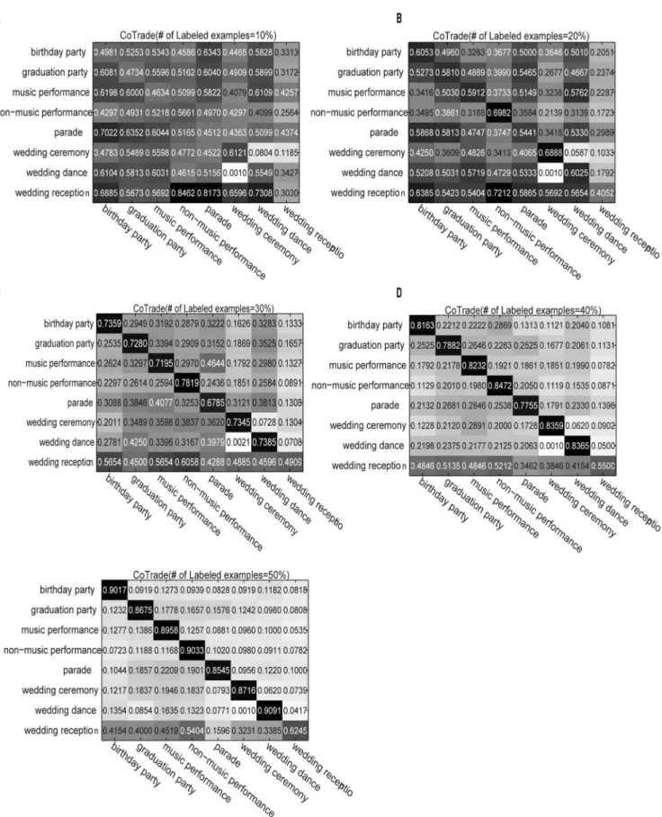
Figure 1. Confusion matrix for CoTrade on the eight activity classes.The subfigures correspond to the performance of the algorithm using different numbers of labeled examples. The x- and y-coordinates are the class labels. (A) Confusion matrix obtained with 10% labeled examples. (B) Confusion matrix obtained with 20% labeled examples. (C) Confusion matrix obtained with 30% labeled examples. (D) Confusion matrix obtained with 40% labeled examples. (E) Confusion matrix obtained with 50% labeled examples.
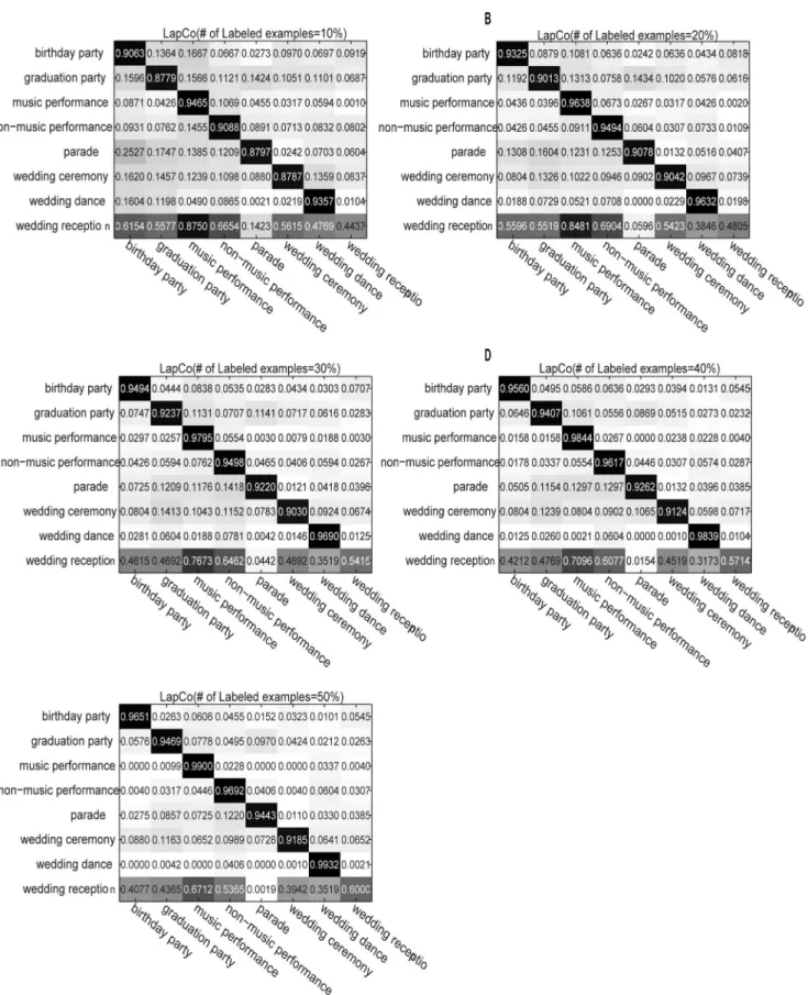
Figure 2. Confusion matrix for LapCo on the eight activity classes.The subfigures correspond to the performance of the algorithm using different numbers of labeled examples. The x- and y-coordinates are the class labels. (A) Confusion matrix obtained with 10% labeled examples. (B) Confusion matrix obtained with 20% labeled examples. (C) Confusion matrix obtained with 30% labeled examples. (D) Confusion matrix obtained with 40% labeled examples. (E) Confusion matrix obtained with 50% labeled examples.
doi:10.1371/journal.pone.0108474.g002
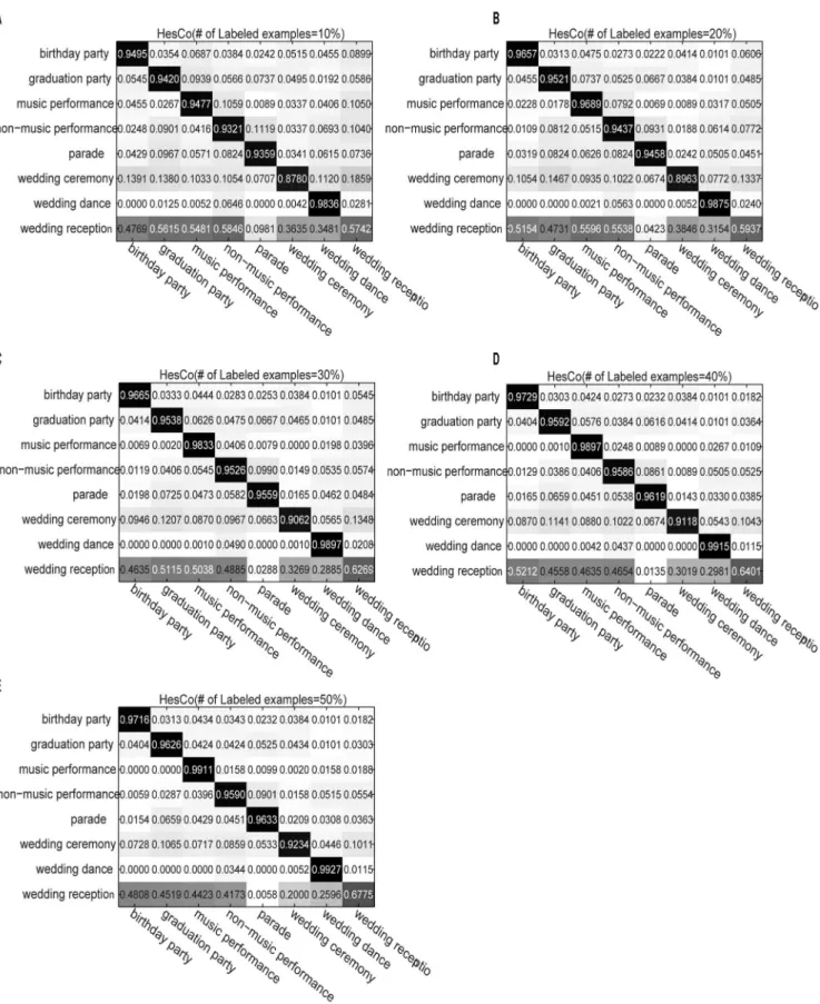
Figure 3. Confusion matrix for HesCo on the eight activity classes.The subfigures correspond to the performance of the algorithm using different numbers of labeled examples. The x- and y-coordinates are the class labels. (A) Confusion matrix obtained with 10% labeled examples. (B) Confusion matrix obtained with 20% labeled examples. (C) Confusion matrix obtained with 30% labeled examples. (D) Confusion matrix obtained with 40% labeled examples. (E) Confusion matrix obtained with 50% labeled examples.
(LapCo). The experimental results demonstrate that the proposed method outperforms the baseline algorithms.
Method Overview
In the standard co-training setting, we are given a two-view training dataset ofN examples, includingllabeled examples, i.e.,
SL~ x1i,x2i,yi
l
i~1, and u unlabeled examples, i.e., SU~ x1i,x2i
N
i~lz1, where x
k
i[Xk for k[f1,2g is the kth view feature vector of theithexample andy
i[f0,1gis the class label of
the ith example (in the remainder of this section we use
xi~ x1i,x2i
to denote theithexample andxk to denote thekth view feature). Labeled examples are drawn fromPand unlabeled examples are drawn from the marginal distributionPX of P, in thatPX is a compact manifoldM. Generally,l%u. The goal of co-training is to predict the labels of unseen examples by learning a hypothesis from the training dataset.
On the other hand, manifold learning assumes that close example pairsxiandxjwill have similar conditional distribution pairs P yDxð iÞ and P yDxj
[28]. It is therefore important to properly exploit the intrinsic geometry of the manifold M that supports PX, and here we employ Hessian regularization to explore the geometry of the underlying manifold. Hessian regularization penalizes the second derivative along the manifold. This approach ensures that the learner is steered linearly along the data manifold, and it is superior to first order manifold learning algorithms, including Laplacian regularization, for both classifica-tion and regression [29] [30] [31]. The effectiveness of Hessian regularization has been well explored by Eells [32], Donoho [21], and Kim [20].
For convenience, we list the important notations used in this paper in Table 1.
In this section, we first briefly introduce Hessian regularization derived from Hessian eigenmaps [21] [20]. We then present the Hessian-regularized support vector machine (HesSVM), which is applied as the classifier for each view of co-training. Finally, we summarize the proposed Hessian regularized co-training.
2.1 Hessian regularization
Given a smooth manifoldM5Rnand the neighborhoodNpat point p[M, the d largest eigenvectors obtained by performing
PCA on the points inNpcorrespond to an orthogonal basis of the tangent spaceTpðMÞ5Rnat pointp[M. We can then define the
Hessian of a function, f :M.R, using the local coordinates. Suppose thatp0[Nphas local coordinatesx. The ruleg xð Þ~f pð Þ0
defines a functiong:U.Ron a neighborhood of 0 inRd. The Hessian of the functionf atpin tangent coordinates can then be
defined as the ordinary Hessian of g by
Htan
f ð Þp
i,j
~ L
Lxi
L Lxj
g xð ÞDx~0. The construction of the tangent
Hessian of a point depends on the choice of the coordinate system used in the underlying tangent space TpðMÞ. Fortunately, the usual Frobenius norm of a Hessian matrix is invariant to coordinate changes [21]. Therefore, we have the Hessian regularizer that measures the average curviness of f along the
manifold M as H fð Þ~Ð
p[M Hftanð Þp 2
Fdp, where
A
k kF~ PijA2
ij 1=2
is the usual Frobenius norm of matrixA. We summarize the computation of Hessian regularization in the following steps [20] [21] [29] [30].
Step 1: Finding thek-nearest neighborsNpof samplexiand form a matrixXiwhose rows consist of the centralized examplesxj{xi for allxj[Np.
Step 2: Estimate the orthonormal coordinate system of the tangent space TxiðMÞ by performing a singular value decomposition of
Xi~UDVT.
Step 3: Performing the Gram-Schmidt orthonormalization process on the matrix Mi~½1 U1 . . . Ud U11 U12 . . . Udd and resultingHi. The Frobenius norm ofHiisHiTHi.
Step 4: Summing upHT
i Hiover all examples and then resulting the Hessian regularizationfTHf.
2.2 The Hessian-regularized support vector machine (HesSVM)
The Hessian-regularized support vector machine (HesSVM) for binary classification takes the form of the following optimization problem:
f~arg min
f[HK
1 l
Xl
i~1
1{yif xð Þi
ð ÞzzcAk kf
2
KzcIfTHf, ð1Þ
where k kf 2K is the classifier complexity penalty term in an appropriate reproducing kernel Hilbert space (RKHS)HK,H is the Hessian matrix, and the termfTHfis the Hessian regularizer to penalizef along the manifoldM. ParameterscAandcIbalance the loss function and the regularization terms, respectively.
According to the representer theorem [28], the solution to problem (1) is given by
f~X lzu
i~1
aiK x,xð iÞ: ð2Þ
By substituting (2) back into (1) and introducing the slack variablesgi for 1ƒiƒl, the primal problem of HesSVM is the following:
a~ arg min a[Rlzu,g[Rl
1 l
Xl
i~1
gizcAaTKazcIaTKHKa
s:t:yi Xl
zu
i~1
ajK xj,xi
zb
!
§1{gi,i~1,. . .,l
gi§0,i~1,. . .,l:
ð3Þ
Figure 4. Mean accuracy (MA) boxplots for the different co-training methods.Each subfigure corresponds to one case of labeled examples. (A) MA obtained using 10% labeled examples. (B) MA obtained using 20% labeled examples. (C) MA obtained using 30% labeled examples. (D) MA obtained using 40% labeled examples. (E) MA obtained using 50% labeled examples.
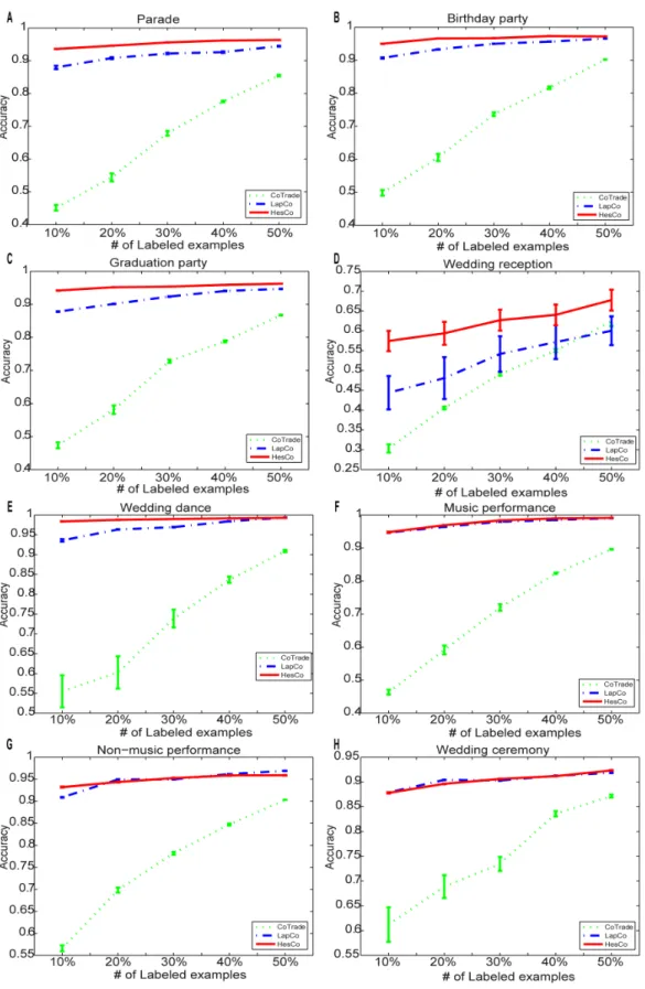
Figure 5. The accuracy of the different methods for the eight activity classes.Each subfigure corresponds to one activity class in the dataset. The x-coordinate is the number of labeled examples. (A) Parade. (B) Birthday party. (C) Graduation party. (D) Wedding reception. (E) Wedding dance. (F) Music performance. (G) Non-music performance. (H) Wedding ceremony.
doi:10.1371/journal.pone.0108474.g005
Using the Lagrangian method, the solution to (3) is
a~ð2cAIz2cIHKÞ{1JTYb, ð4Þ
whereJ~½I his anl|ðlzuÞmatrix withIas thel|lidentity matrix andhas thel|uzero matrix,Y~diag y1,y2,ð . . .,ylÞ, and bis the solution to the following problem:
b~arg min b[Rl
Xl
i~1
bi{1
2b
TQb
s:t:X
l
i~1
biyi~0
1ƒbiƒ1
l,i~1,. . .,l,
ð5Þ
where Q~YJKð2cAIz2cIHKÞ{1JTY, J~½I h is the
l|ðlzuÞmatrix,I is thel|lidentity matrix,his thel|uzero matrix, andY~diag y1,y2,ð . . .,ylÞ.
Problem (3) can then be transformed into a standard quadratic programming problem (5) that can be solved using an SVM solver.
2.3 Hessian regularized co-training (HesCo)
Similar to standard co-training algorithms, HesCo also itera-tively learns the classifiers from the labeled and unlabeled training examples. In each iteration, HesSVM exploits the local geometry to significantly boost the prediction of unlabeled examples, which helps to effectively augment the training set and update the classifiers. Table 2 summarizes the procedure of HesCo by integrating HesSVM into CoTrade [33].
2.4 Complexity analysis
Suppose we are given n examples, the computation of the inverse of a dense Gram matrix leads to O n 3
and general HesSVM implementations typically have a training time com-plexity that scales between O nð Þ and O n 2:3
. Hence in each iteration of co-training, the time cost is approximately O n 3
. Denote the number of iteration asg, the total cost of the proposed method is aboutgO n 3
.
Experiments
We conducted experiments for social activity recognition on the USAA database [22] [23]. The USAA database is a subset of the CCV database [34] and contains eight different semantic class videos, as described above.
In our co-training experiments, we used tagging features as one view and visual features as the other. The tagging features are the 69 ground-truth attributes provided by Fu et al. [22] [23], and the visual features are low features that concatenate SIFT, STIP, and MFCC according to [34].
We used the same training/testing partition as in [22] and [23], in which the training set contains 735 videos and the testing set contains 731 videos. Each class contains around 100 videos for training and testing, respectively. In our experiments, we selected any two of the eight classes to evaluate performance, resulting in a
total of 28 one vs. one binary classification experiments. We randomly divided the training set 10 times to examine the robustness of the different methods. In each experiment, we selected 10%, 20%, 30%, 40%, and 50% of the training videos as labeled examples, and the rest as unlabeled examples, for initialization assignment. ParameterscA andcI in HesSVM and
LapSVM were tuned using the candidate set
10eDe~{10,{9,
. . .,9,10
f g. The parameter k, which denotes
the number of neighbors when computing the Hessian and graph Laplacian, was set to 100.
We compared the proposed HesCo with CoTrade and Laplacian regularized co-training (LapCo). The accuracy and mean accuracy (MA) for all classes were used as assessment criteria.
Figure 1 shows the confusion matrix for the CoTrade method on the eight social activity classes. The subfigures correspond to the performance of the algorithm using different numbers of labeled examples. The x- and y-coordinates are the class labels. Figures 2 and 3 similarly demonstrate the performances of LapCo and HesCo, respectively. From Figure 1 we can see that the errors are distributed across the category labels when there are only a few labeled examples, and from Figures 2 and 3 we can see that LapCo and HesCo significantly improve performance, especially when the number of labeled examples is small.
Figure 4 shows the MA boxplots for the different co-training methods, with each subfigure corresponding to one case of labeled examples. LapCo and HesCo both perform better than CoTrade, and HesCo outperforms LapCo.
Figure 5 shows the accuracy of the different methods for the eight activity classes. Each subfigure corresponds to one activity class in the dataset, and the x-coordinate is the number of labeled examples. Manifold regularized co-training methods, including LapCo and HesCo, significantly boost performance for every activity class, especially when the number of labeled examples is small. HesCo outperforms LapCo in most cases.
Conclusion
Here we propose Hessian regularized co-training (HesCo) to boost co-training performance. In this method, each Hessian is first obtained from a particular view of examples. Second, Hessian regularization is used to explore the local geometry of the underlying manifold for the training of the classifier. Hessian regularization significantly boosts the performance of the learners and then improves the effectiveness of augmenting the training set in each co-training round. Comprehensive experiments on social activity recognition in the USAA dataset were conducted to evaluate the proposed HesCo algorithm, which demonstrated that HesCo outperforms baseline methods, including the traditional co-training algorithm and Laplacian regularized co-co-training, espe-cially with small numbers of labeled examples.
Author Contributions
Conceived and designed the experiments: WL YL DT YW. Performed the experiments: WL YL XL. Analyzed the data: WL YL DT YW. Contributed reagents/materials/analysis tools: WL YL DT YW. Contrib-uted to the writing of the manuscript: WL YL DT YW. Baseline evaluations: WL XL.
References
1. Zhang L, Zhen X, Shao L (2014) Learning Object-to-Class Kernels for Scene Classification. IEEE Trans. Image Process, 23(8): 3241–3253.
2. Yan R, Shao L, Liu Y (2013) Nonlocal Hierarchical Dictionary Learning Using Wavelets for Image Denoising. IEEE Trans. Image Process, 22(12): 4689–4698.
4. Tao D, Li X, Wu X, Maybank S J (2007) General Tensor Discriminant Analysis and Gabor Features for Gait Recognition. IEEE Trans. Pattern Anal. Mach. Intell., 29(10): 1700–1715.
5. Blum A, Mitchell T (1998) Combining labeled and unlabeled data with co-training. Proceedings of the 11th ACM annual conference on Computational learning theory: 92–100.
6. Song M, Tao D, Huang X, Chen C, Bu J (2012) Three-dimensional face reconstruction from a single image by a coupled RBF network. IEEE Trans. Image Process, 21(5): 2887–2897.
7. Song M, Tao D, Sun S, Chen C, Bu J (2013) Joint Sparse Learning for 3-D Facial Expression Generation. IEEE Trans. Image Process, 22(8): 3283–3295. 8. Song M, Chen C, Bu J, Sha T (2012) Image-based facial sketch-to-photo
synthesis via online coupled dictionary learning. Information Sciences, 193: 233–246.
9. Zhu F, Shao L (2014) Weakly-Supervised Cross-Domain Dictionary Learning for Visual Recognition. International Journal of Computer Vision (IJCV), 109(1–2): 42–59.
10. Xu C, Tao D, Xu C (2013) A Survey on Multi-view Learning. arXiv:1304.5634. 11. Xu C, Tao D, Xu C (2014) Large-Margin Multi-view Information Bottleneck.
IEEE Trans. Pattern Anal. Mach. Intell. 36(8): 1559–1572.
12. Nigam K, Ghani R (2000) Analyzing the effectiveness and applicability of co-training. Proceedings of the ninth international conference on Information and knowledge management: 86–93.
13. Brefeld U, Scheffer T (2004) Co-EM Support Vector Learning. Proceedings of the twenty-first international conference on Machine learning: 16.
14. Zhou Z, Li M (2005) Semi-Supervised Regression with Co-Training. International Joint Conference on Artificial Intelligence: 908–916.
15. Brefeld U, Ga¨rtner T, Scheffer T, Wrobel S (2006) Efficient co-regularised least squares regression. Proceedings of the 23rd ACM international conference on Machine learning: 137–144.
16. Sindhwani V, Niyogi P, Belkin M (2005) A co-regularization approach to semi-supervised learning with multiple views. Proceedings of ICML workshop on learning with multiple views: 74–79.
17. Kumar A, Rai P, Daume´ III H (2010) Co-regularized spectral clustering with multiple kernels. Proceedings of NIPS Workshop: New Directions in Multiple Kernel Learning.
18. Kumar A, Rai P, Daume´ III H (2011) Co-regularized Multi-view Spectral Clustering. Adv. Neural Inf. Process Syst.: 1413–1421.
19. Kumar A, Daume´ III H (2011) A Co-training Approach for Multi-view Spectral Clustering. Proceedings of the 28th International Conference on Machine Learning: 393–400.
20. Kim KI, Steinke F, Hein M (2009) Semi-supervised Regression using Hessian Energy with an Application to Semi-supervised Dimensionality Reduction. Adv. Neural Inf. Process Syst. 22: 979–987.
21. Donoho DL, Grimes C (2003) Hessian Eigenmaps: new locally linear embedding techniques for high-dimensional data. Proceedings of the National Academy of Sciences, 100(10): 5591–5596.
22. Fu Y, Hospedales T, Xiang T, Gong S (2012) Attribute Learning for Understanding Unstructured Social Activity-annotated. Paper presented at the European Conference on Computer Vision.
23. Fu Y, Hospedales T, Xiang T, Gong S (2014) Learning Multi-modal Latent Attributes. IEEE Trans. Pattern Anal. Mach. Intell., 36(2): 303–316. 24. Shao L, Jones S, Li X (2014) Efficient Search and Localization of Human
Actions in Video Databases, IEEE Trans Circuits Syst. Video Technol., 24(3): 504–512.
25. Liu L, Shao L, Zheng F, Li X (2014) Realistic Action Recognition via Sparsely-Constructed Gaussian Processes. Pattern Recognition, doi:10.1016/j.patcog. 2014.07.006.
26. Zhang Z, Tao D (2012) Slow Feature Analysis for Human Action Recognition, IEEE Trans. Pattern Anal. Mach. Intell., 34(3): 436–450.
27. Tao D, Jin L, Wang Y, Yuan Y, Li X (2013) Person Re-Identification by Regularized Smoothing KISS Metric Learning. IEEE Trans. Circuits Syst. Video Techn. 23(10): 1675–1685.
28. Belkin M, Niyogi P, Sindhwani V (2006) Manifold Regularization: A Geometric Framework for Learning from Labeled and Unlabeled Examples. Journal of Machine Learning Research, 7: 2399–2434.
29. Liu W, Tao D (2013) Multiview Hessian Regularization for Image Annotation. IEEE Trans. Image Process, 22(7): 2676–2687.
30. Tao D, Jin L, Liu W, Li X (2013) Hessian Regularized Support Vector Machines for Mobile Image Annotation on the Cloud. IEEE Trans. on Multimedia, 15(4): 833–844.
31. Liu W, Tao D, Cheng J, Tang Y (2014) Multiview Hessian discriminative sparse coding for image annotation. Comput. Vis. Image Underst., 118: 50–60. 32. Eells J, Lemaire L (1983) Selected Topics in Harmonic Maps, University of
Warwick, Mathematics Institute.
33. Zhang M, Zhou Z (2011) COTRADE: Confident Co-Training With Data Editing. IEEE Trans. Syst. Man Cybern. B Cybern., 41(6): 1612–1626. 34. Jiang Y, Ye G, Chang S, Ellis D, Loui AC (2011) Consumer Video
Understanding: A Benchmark Database and An Evaluation of Human and Machine Performance. Proceedings of the 1st ACM International Conference on Multimedia Retrieval: 19.