Comparison of Hybrid Classifiers for Crop
Classification Using Normalized Difference
Vegetation Index Time Series: A Case Study
for Major Crops in North Xinjiang, China
Pengyu Hao1,2, Li Wang1*, Zheng Niu1
1The State Key Laboratory of Remote Sensing Science, Institute of Remote Sensing and Digital Earth, Chinese Academy of Sciences, Beijing, 100101, China,2University of Chinese Academy of Sciences, Beijing, 100049, China
Abstract
A range of single classifiers have been proposed to classify crop types using time series vegetation indices, and hybrid classifiers are used to improve discriminatory power. Traditional fusion rules use the product of multi-single classifiers, but that strategy cannot integrate the classification output of machine learning classifiers. In this research, the per-formance of two hybrid strategies, multiple voting (M-voting) and probabilistic fusion (P-fusion), for crop classification using NDVI time series were tested with different training sample sizes at both pixel and object levels, and two representative counties in north Xinjiang were selected as study area. The single classifiers employed in this research included Random Forest (RF), Support Vector Machine (SVM), and See 5 (C 5.0). The results indicated that classification performance improved (increased the mean overall accuracy by 5%~10%, and reduced standard deviation of overall accuracy by around 1%) substantially with the training sample number, and when the training sample size was small (50 or 100 training samples), hybrid classifiers substantially outperformed single classifiers with higher mean overall accuracy (1%~2%). However, when abundant training samples (4,000) were employed, single classifiers could achieve good classification accuracy, and all classifiers obtained similar performances. Additionally, although object-based classifica-tion did not improve accuracy, it resulted in greater visual appeal, especially in study areas with a heterogeneous cropping pattern.
Introduction
Crop-type information is important for the global food security system, and there is an urgent demand for accurate crop classification data [1–3]. Since the crop calendar varies among differ-ent crops, phenology is the basis of crop classification [4]. Vegetation indices (VI), which could be calculated from remote sensing images, can measure vegetation coverage, and VI time series OPEN ACCESS
Citation:Hao P, Wang L, Niu Z (2015) Comparison of Hybrid Classifiers for Crop Classification Using Normalized Difference Vegetation Index Time Series: A Case Study for Major Crops in North Xinjiang, China. PLoS ONE 10(9): e0137748. doi:10.1371/ journal.pone.0137748
Editor:Quazi K. Hassan, University of Calgary, CANADA
Received:November 18, 2014
Accepted:August 20, 2015
Published:September 11, 2015
Copyright:© 2015 Hao et al. This is an open access article distributed under the terms of theCreative Commons Attribution License, which permits unrestricted use, distribution, and reproduction in any medium, provided the original author and source are credited.
Data Availability Statement:All relevant data are within the paper and its Supporting Information files.
Funding:This study was supported by the National Natural Science Foundation of China (41371358) and (41301498).
can describe crop phenology [5–7]. Thus, VI time series have been employed widely to produce crop classification data [8–12]. In addition, the Normalized Difference Vegetation Index (NDVI) has the higher importance score than other features, such as multi-spectral bands, cal-culated indices and ancillary data [13].
Coarse spatial resolution data, such as Moderate Resolution Imaging Spectroradiometer (MODIS) (250–500m) data, are characterized by high temporal resolution and have shown potential for identifying crops [14,15]. However, one drawback is that the spatial resolution of MODIS data is relatively coarse, and the classification accuracy is affected by mixed pixels when the field size is small. For sensors at finer spatial resolution, such as Landsat-5/7 TM/ ETM+ (at 30-m resolution), the revisit period is relatively long (e.g., 16days for Landsat). Thus, Landsat cannot provide enough cloud-free imagery for most regions of the world [16]. As some other sensors (such as Huan Jing and DEIMOS) can provide images at medium spatial resolution [17,18], the use of multi-sensor merged image time series has improved the perfor-mance of crop identification at medium resolution [19,20].
A range of classifiers, such as Decision Tree (DT), Support Vector Machine (SVM), Ran-dom Forest (RF), and C5 [14,21,22], have been employed for crop type classification. In addi-tion, totake advantage of single classifiers and increase the classifiers’discriminatory power, some hybrid classifiers have been proposed based on product and sum rules [23]. For example, Du, Chang [24] mixed Spectral Information Divergence (SID) and Spectral Angle Mapper (SAM) and Ghiyamat and Shafri [25] mixed SID and Spectral Correlation Measure (SCM) uti-lizing product rules, and the mixed classifiers have shown good performance in hyperspectral classification. However, a drawback is that the improvement of the product rule is limited when multiple (more than three) classifiers are used. Various other hybrid strategies, such as the multi-classifier approaches multiple voting (M-voting) and probabilistic fusion (P-fusion), have been employed to combine the classification results obtained from multi-spectral and tex-tual features and have improved the performance of the classification [26]. However, few stud-ies have tested the performance of multi-classifier systems on integrating classifiers.
Pixel-based image analyses (PBIA) have led to some misclassifications, which are due mainly to 1) the similar spectral characteristics of some crop classes, 2) the spectral variability due to the canopy and bare soil background reflectance and different crop development sched-ules, and 3) the mixed pixels located at the boundaries between classes [8]. Object-based image analyses (OBIA) were proposed to solve these problems [13], and a number of studies have found that OBIA methods are effective for classification for both high- and moderate-resolu-tion imagery [27]. In addition, several studies have compared the performance of OBIA with that of PBIA. For images with high spatial resolution (spatial resolution better than 10 m), OBIA outperformed PBIA with better classification accuracy and the capacity to extract patch boundaries [28,29]. At medium spatial resolution (10–100m), OBIA generally provides a visu-ally appealing appearance, but conclusions about statistical accuracy have varied. Some studies have shown that OBIA achieved higher classification accuracy than PBIA [30,31]; some obtained the opposite conclusion, PBIA obtaining better accuracy [32,33]; and others con-cluded that OBIA and PBIA acquired similar classification accuracy [34,35]. Thus, additional study remains essential to test the potential of OBIA in improving the classification of specific crop classes.
[17]; 2) compare the performance of hybrid strategies (M-voting and P-fusion) with the single classifiers for crop classification; and 3) compare the performance of OBIA and PBIA for crop classification.
Study Regions and Data Description
Description of the study area and crop calendar
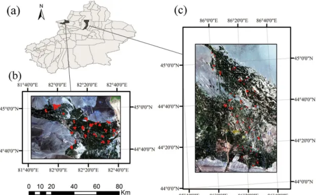
In this research, we selected two representative agricultural regions in northern Xinjiang: one located in Bole County, which has 32 kha of cropland (44°200–45°230N, 80°400–82°420E), a sec-ond located in Manas County, which covers 180 kha of cropland (43°170–45°200N, 85°170–86° 460E) (Fig 1). The regions have a temperate continental climate characterized by dryness and drought. The annual average temperature and rainfall are 7.0°C and 202mm in Bole and 7.2°Cand 208mm in Manas, respectively.
The dominant crops grown in the study areas include cotton, maize (spring maize and sum-mer maize), watermelon, grape, tomato, and wheat. The vegetation cover fraction for each crop type over the growing season is presented inFig 2. Cotton, spring maize, watermelon, tomato, and grape are planted in early April and begin their growth mostly during the June–July period. For harvest, watermelon and tomato are harvested in August, spring maize is harvested in early September, and grapes and cotton are harvested during the August–September and Septem-ber–October periods. Winter wheat is planted in early November, begins its growth in the next April, and is reaped for harvest in late June. After that, some fields are in rotation, and others are planted to summer crops such as summer maize. Thus, we divided the winter wheat into two classes depending on whether summer crops are planted in the same field or not.
Fig 1. Study areas: (a) Location of Bole and Manas in Xinjiang and extent of Xinjiang. (b) Bole (2011/7/11) and (c) Manas (2011/7/13).The red patterns on the images are distributions of ground reference data.
Datasets
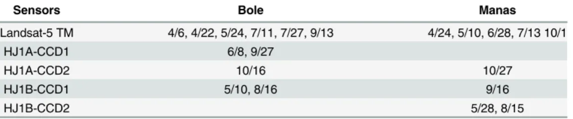
Satellite images and vegetation indices. We selected cloud-free (cloud cover less than 20%) satellite images in both study regions covering the entire growing season (Table 1), including both the Landsat TM CDR land surface reflectance product and the Huan Jing (HJ) CCD level 2 product of 2011 [36]. The HJ-1 satellite constellation, launched by the Chinese Government in 2008, has two CCD cameras that observe a broad coverage of 720 km and have spatial resolution of 30m. The CCD cameras have four visible and near-infrared bands, which include B1 (0.43–0.52nm), B2 (0.52–0.60nm), B3 (0.63–0.69nm), and B4 (0.76–0.9nm) [37]. In this research, we intended to obtain a NDVI time series at 30-m spatial resolution and at approximately 15-day temporal resolution during the growing season. However, TM images cannot cover the entire growing season of the study areas at such a high temporal resolution. Therefore, we employed cloud-free Landsat TM and HJ CCD (with similar spatial resolution to Landsat TM) images to build the image time series. All HJ images were georeferenced to the UTM WGS84 zone 44N (Bole) and 45N (Manas), and the HJ images were then registered to the TM images, achieving an RMSE of less than 0.3 pixels using a second-order polynomial transformation and B-linear resampling. Then, radiance calibration and Fast Line-of-sight Atmospheric Analysis of Hypercubes (FLAASH) atmospheric correction were performed using Environment for Visualizing Images (ENVI) for all images [38–40]. NDVI was calculated using the reflectance of visible (red) and near-infrared (NIR) bands for both TM and HJ images using Eq (1).
NDVI¼rðNIRÞ rðRedÞ
rðNIRÞ þrðRedÞ ð1Þ
Ground reference data. Ground-truth data were obtained by fieldwork in the study regions during 2011. Fields were selected to represent the full variety of crop types and an even distribution across the study areas. The selected fields, 457 fields in Bole and 435 fields in Manas, were then surveyed. For each field, the crop type was collected as attribute information. Field boundaries were recorded using GPS and digitized as polygons in ArcGIS. To avoid
Fig 2. Vegetation cover fraction of crop types within the annual growing season.
doi:10.1371/journal.pone.0137748.g002
Table 1. TM and HJ-1 CCD images for both study regions.
Sensors Bole Manas
Landsat-5 TM 4/6, 4/22, 5/24, 7/11, 7/27, 9/13 4/24, 5/10, 6/28, 7/13 10/1
HJ1A-CCD1 6/8, 9/27
HJ1A-CCD2 10/16 10/27
HJ1B-CCD1 5/10, 8/16 9/16
HJ1B-CCD2 5/28, 8/15
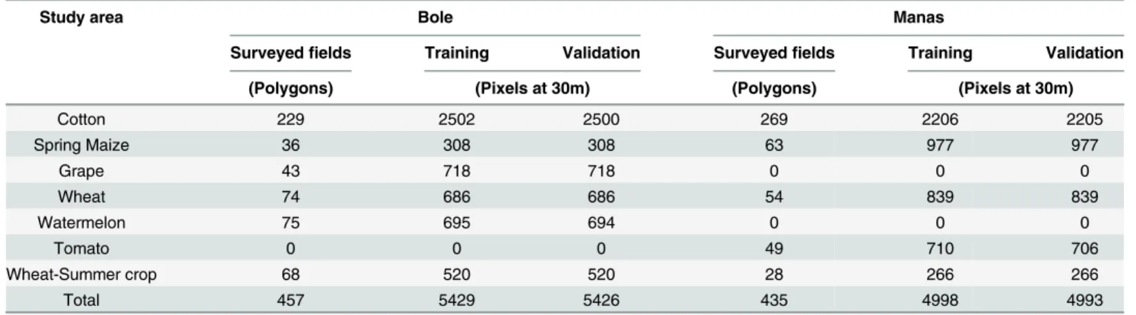
boundary pixels, polygons were converted to a raster format using the TM grid. In total, 10,855 sample pixels for Bole and 9,991 pixels for Manas were obtained. The distribution of ground-truth data is shown inFig 1. The amounts of training and validation samples for each crop type are shown inTable 2, and the training and validation dataset are provided inS1 Dataset.
Methods
The methodology of the study is presented inFig 3. First, we measured the consistency between Landsat TM NDVI and HJ CCD NDVI, and then utilized Landsat TM and HJ CCD images to
Table 2. Number of training and validation samples.
Study area Bole Manas
Surveyedfields Training Validation Surveyedfields Training Validation
(Polygons) (Pixels at 30m) (Polygons) (Pixels at 30m)
Cotton 229 2502 2500 269 2206 2205
Spring Maize 36 308 308 63 977 977
Grape 43 718 718 0 0 0
Wheat 74 686 686 54 839 839
Watermelon 75 695 694 0 0 0
Tomato 0 0 0 49 710 706
Wheat-Summer crop 68 520 520 28 266 266
Total 457 5429 5426 435 4998 4993
doi:10.1371/journal.pone.0137748.t002
Fig 3. Methodology of the study.
build time series NDVI covering the entire growing season. Then, we used the single classifiers to classify crop types and obtained both a classification map and probabilistic outputs for each classifier. Afterward, the performance of two fusion strategies, M-voting and P-fusion, at both pixel and object levels were assessed using both statistical and visual analyses. The training sample size varied from 50 to 4000 (50, 100, 250, 500, 750, 1000, 1500, 2000, 2500, 3000, 3500, and 4000) in each study area, and for each training sample size, the samples were randomly selected from the training sample set listed inTable 2. Additionally, all classifiers were trained ten times for each training sample size, and both the average and standard deviation of the clas-sification accuracy were reported.
Similarity Measure between Landsat and HJ NDVI
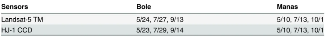
We evaluated the NDVI consistency between Landsat-5 TM and HJ-1 CCD data by comparing the NDVI of the two sensors for similar dates (Table 3). To reduce the potential impacts of reg-istration inaccuracy, we defined subsets of homogeneous regions of interest (ROI) with 3 × 3 windows located in the middle of larger homogeneous“patches”[41]. Average values of these sampling windows were used to compare the consistency between Landsat-5 TM and HJ-1 CCD NDVI. Through this process, we defined subsets of the ROIs for different crop types, selecting 170 and 153 windows within Bole and Manas, respectively. Scatter plots and linear relationships were used to examine how Landsat-5 TM and HJ-1 CCD NDVI differed in performance.
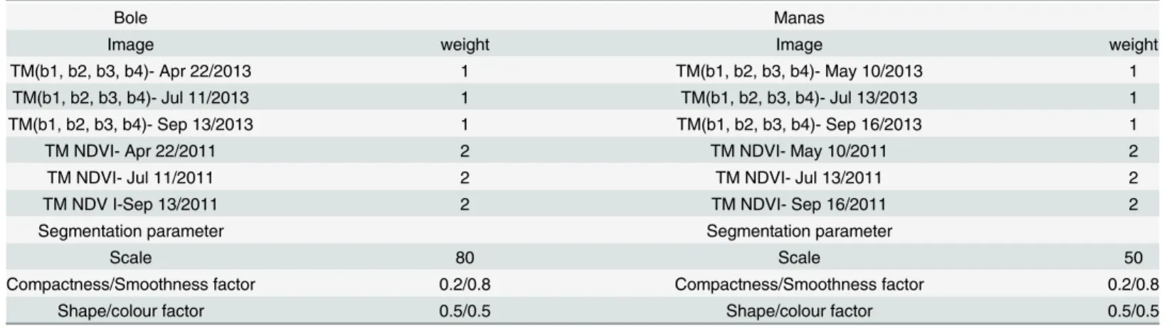
Image segmentation
To compare the performances of different classifiers at pixel and object level, we segmented the image using the multi-resolution segmentation (MRS) algorithm of eCognition [42]. The MRS algorithm is a“bottom-up”approach that begins with pixel-sized objects and iteratively grows through the pair-wise merging of neighboring objects based on several user-defined parame-ters, including scale, color/shape, weights of spectral bands, and smoothness/compactness [42]. Landsat images of three time periods were used during the segmentation process in both of the study regions; and a summary of the segmentation parameters used is presented inTable 4.
Classifiers
Single classifiers. The performances of the following three single classifiers were evalu-ated: 1) Random Forest (RF), 2) Support Vector Machine (SVM), and 3) C 5.0 Rule-Based Model (C5.0). SVM is a non-parametric supervised classifier derived from statistical learning theory [10]. In the simplest form, SVMs are linear binary classifiers that label a given test sam-ple from one of the two possible classes. The classifiers use training samsam-ples to find the optimal hyperplanes that separate classes with minimum classification error. Significantly, only the training samples that lie on the margin (called support vectors) are used to define the hyper-planes. The simplest SVMs assume that the problems are linearly separable. However,“data points”of different classes overlap in practice. As a result, the basic linear decision boundaries cannot classify patterns with high accuracy. Thus, the linearly inseparable problems are solved
Table 3. Images used for consistency measurement for both study areas.
Sensors Bole Manas
Landsat-5 TM 5/24, 7/27, 9/13 5/10, 7/13, 10/1
HJ-1 CCD 5/23, 7/29, 9/14 5/10, 7/13, 10/1
by transforming the nonlinear correlations into a higher (Euclidean or the Hilbert) space using a kernel function [21]. Another problem is that remote sensing classifications always involve multi-class situations. In this case, the binary classifier (simplest SVM) is used as a multi-class classifier based on one-against-one and one-against-others methods [21,43]. Generally, SVM is not based on the assumption that the data are normally distributed for a particular image; thus, SVM could outperform classifiers based on maximum likelihood theory [10]. Addition-ally, SVM has the advantages of being able to deal with high-dimensional datasets and small training samples [44–46], and SVM has been utilized widely for crop classification [10,20,47]. In this study, implementation of SVM was performed with the libSVM (library e1071 for R) [48].The widely used radial basis function kernel (RBF) was selected, and the data space was normalized to a common scale [0, 1]. In addition, training of the SVM included choosing a ker-nel parameter“γ”(gamma) and a regularization parameter“C”(cost).“C”controls the penalty
associated with misclassified training samples, and“γ”determines the gamma of the kernel
function [49]. Then, the parameters“C”and“γ”were selected using a systematic 2-D space
spanned by“γ”and“C”.
The RF algorithm is an ensemble machine learning technique that combines multiple trees [22]. Each tree is constructed using two-thirds of the original cases. Then, the remaining one-third of the cases are employed to generate a test classification, with an error referred to the “out-of-bag error”(OOB error). Subsequently, the model output is determined by the majority vote of the classifier ensemble [50]. Two free parameters can be optimized in the RF algorithm: the number of trees (ntree) and the number of features to split the nodes (mtry). The advan-tages of the RF algorithm, such as the relatively high efficiency with large datasets, the probabil-ity output for each class, and the generated OOB error (an internal unbiased estimate of the generalization error), make it suitable for remote sensing applications [51]. In this study, both the crop-label and probabilistic output were obtained using the Random Forest library for R [52]. The“ntree”parameter was set to a relatively high value of 1000 to allow convergence of the OOB error statistic, and“mtry”was set to the square root of the total number of input fea-tures [53].
C5.0 is a decision tree algorithm developed from C4.5. In C4.5, when training the model, all training samples are set as the root of the decision tree. Then, the gain information ratio of every feature is calculated based on the entropy of the feature, and the feature with the highest information gain is selected to split the data into multi-subsets. The algorithm repeats this pro-cedure on each subset until all instances in the subset belong to the same class and a leaf node is created [27,54]. C5.0 advanced C4.5 by the development of a boosting technique (generating
Table 4. Summary of variables and parameters used in the segmentation.
Bole Manas
Image weight Image weight
TM(b1, b2, b3, b4)- Apr 22/2013 1 TM(b1, b2, b3, b4)- May 10/2013 1
TM(b1, b2, b3, b4)- Jul 11/2013 1 TM(b1, b2, b3, b4)- Jul 13/2013 1
TM(b1, b2, b3, b4)- Sep 13/2013 1 TM(b1, b2, b3, b4)- Sep 16/2013 1
TM NDVI- Apr 22/2011 2 TM NDVI- May 10/2011 2
TM NDVI- Jul 11/2011 2 TM NDVI- Jul 13/2011 2
TM NDV I-Sep 13/2011 2 TM NDVI- Sep 16/2011 2
Segmentation parameter Segmentation parameter
Scale 80 Scale 50
Compactness/Smoothness factor 0.2/0.8 Compactness/Smoothness factor 0.2/0.8
Shape/colour factor 0.5/0.5 Shape/colour factor 0.5/0.5
and combining multiple classifiers to improve predictive accuracy) [55]. C5.0 has several advantages including that it is fast to train and it has a set of rules. Thus, it has been employed widely in land use and land cover classification (LULC) [56,57]. In this study, C5.0 was imple-mented using the library C50 for R [58], and the parameters“trails”that specify the number of boosting iterations was set at 10.
Uncertainty of the classification result obtained from the single classifier. All three sin-gle classifiers employed in this research can provide the probabilistic output, (p1(x), , pk(x), , pK(x), k = 1, 2, , K), which can reflect the classification uncertainty of the classifier. In
this paper, we used theαquadratic entropy to calculate the uncertainty [59], as in Eq (2):
HðpðxÞÞ ¼ 1
n2 2a
XK k¼1p
a
kðxÞð1 pkðxÞÞ a
ð2Þ
where H(p(x)) represent theαquadratic entropy of the vector p(x), p1(x), , pk(x), , pK(x)
represent the probabilistic outputs. While,αis user-defined value which ranges from 0 and 1,
andα= 0.5 was chosen in this study. A smaller H(p(x)) indicates a more reliable classification.
The advantage of the specificity measure is that it applies all the information in the probability vector.
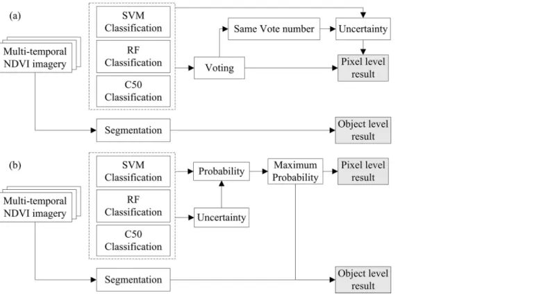
Hybrid strategies: Voting and fusion. We used two hybrid strategies (multiple voting, M-voting and probabilistic fusion, P-fusion) to integrate single classifiers and then compared their performance with that of the single classifiers [26]. Processing chains of the voting and fusion strategies are shown inFig 4.
In M-voting, each single classifier has a vote, and if a class obtains more votes than all the other classes, the pixel is labeled as the class with the most votes.
CðxÞ ¼maxk¼f1;;KgVxðkÞ ð3Þ
where C(x) is the label of the pixel x and Vx(k) is the number of votes that pixel x received for
class k. Otherwise, if the votes that two or more classes obtained are the same, the classification uncertainty of the single classifiers were compared. And the pixel is labeled as the class of the single classifier with the least classification uncertainty:
CðxÞ ¼Cðx^fÞwith^f ¼minf¼f1;;FgSfðxÞ ð4Þ
where Sf(x) is the classification uncertainty of pixel x with classifier f, which is the H(p(x))
cal-culated by Eq (2) in this study. And^f is the optimal classifier with the least classification uncer-tainty. For M-voting at the object level, a similar algorithm is employed. All pixels in an object could vote for thefinal label of the object, and the object is labeled as the class with the most votes as in Eq (3).
In P-fusion, the probabilistic and uncertainty results of single classifiers are utilized to define the classification label C(x), as in Eq (5):
CðxÞ ¼maxk¼f1;;Kg
XF
f¼1 pk
fðxÞ
SfðxÞ
ð5Þ
where pk
fðxÞis the probabilistic value of pixel x for class k with classifier f. Sf(x) is the
Metric for classifier approach comparison
Along with the commonly used accuracy assessment indices, including producer’s accuracy (PA), user’s accuracy (UA), overall accuracy (OA), and kappa coefficient (kappa), calculated from the error matrix [60], McNemar’s test was employed in this study to evaluate the statisti-cal significance of the accuracy of the different classifiers [61]. McNemar’s test is a non-parametric test based on the standardized normal test statistic, as in Eq (6):
Z¼ f12 f21 ffiffiffiffiffiffiffiffiffiffiffiffiffiffiffiffi f12þf21
p ð6Þ
where f12is the number of samples that are correctly classified by classifier 1 and incorrectly
classified by classifier 2. We defined three cases of differences in accuracy between classifier 1 and classifier 2 according to McNemar’s test:
1. No significance between classifiers 1 and 2 (N):−1.96Z1.96;
2. Positive significance (classifier 1 has higher accuracy than classifier 2) (S+): Z>1.96;
3. Negative significance (classifier 1 has lower accuracy than classifier 2) (S-): Z<−1.96.
Results
Similarity Measure between Landsat and HJ NDVI
Three matching images (acquired in May, July and September) were used to measure the con-sistency between Landsat-5 TM and HJ-1 CCD NDVI in both study areas. The scatter plots and linear relationships of the NDVI for the matching images are shown inFig 5. In both study
Fig 4. Processing chains of (a) M-voting and (b) P-fusion for the hybrid classifiers.
areas, the R2values were larger than 0.9 for the NDVI of all the time periods. In addition, the fitted lines between Landsat-5 NDVI and HJ-1 NDVI were close to the 1:1 line. These results coincided with those of previous research and indicated that Landsat-5 TM and HJ-1 CCD data had a strong linear relationship [62–65]. Overall, the HJ-1 CCD andLandsat-5 TM images had similar spatial resolution and high NDVI consistency. Therefore, NDVI from both sensors was utilized to obtain the time series for this research.
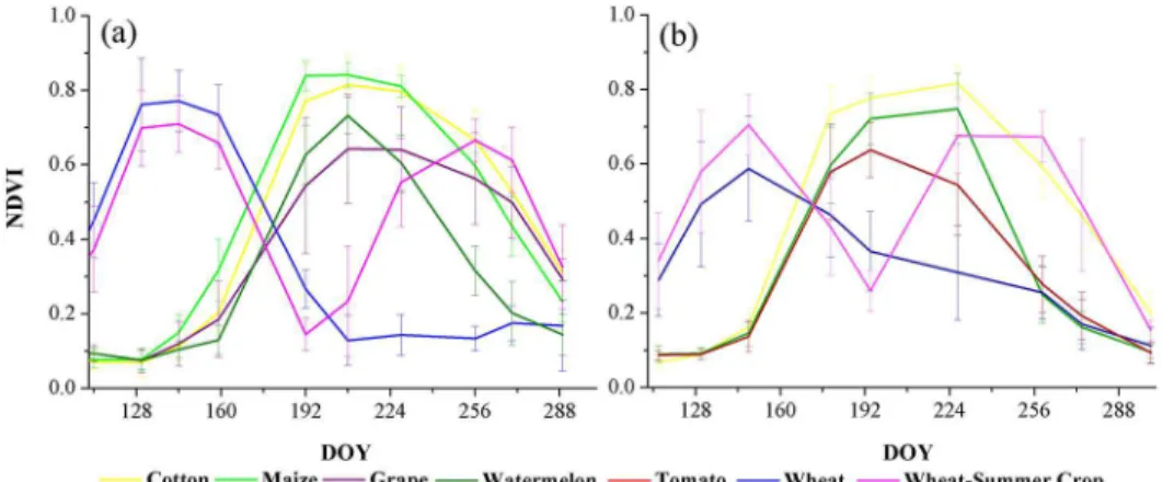
The NDVI time series of the major crops in both study areas are shown inFig 6. Cotton was the major crop, and the highest NDVI value of cotton was between 0.7 and 0.9 around day 200 (early August). For spring maize, the highest value was similar to that of cotton, but after the peak, NDVI of spring maize decreased faster than that of cotton, and at around day 250 (Sep-tember), the NDVI of spring maize was relatively lower than the value for cotton. Similar to cotton, the NDVI peaks of tomato and watermelon were around day 200, but the NDVI values were between 0.6 and 0.7, significantly lower than those of cotton and spring maize. For grape, NDVI was high during days 170–270 (from late June to late September). In addition, the
Fig 5. Scatter plots of NDVI data from HJ-1 CCD andLandsat-5 TM images.Note: The red lines are the 1:1 lines, and the dashed lines are fitted lines of HJ-1 NDVI and Landsat-5 NDVI.
NDVI of grape had the largest variability among all crops in the study region (between 0.4 and 0.7). The major winter crop in the study areas was winter wheat, and the time period of high NDVI (above 0.5) was between day 120 and day 130.
Accuracy assessment of classification result
The producer’s accuracy (PA), user’s accuracy (UA), and overall accuracy (OA) of the different classifiers with different training sample sizes are presented in Tables5–8, respectively, and the results (mean and standard deviation (SD) of the accuracy) are reported based on ten runs of different training sample sets.
In Bole, when the training sample number was 100, SVM obtained the highest mean OA (79.26%), C5.0 had the lowest mean OA (77.2%) among the three single classifiers; and SVM and RF had similar overall accuracy SD (around 1.8%) which was slightly lower than that of C5.0 (1.92%). Among the major crops in Bole, wheat and wheat-to-summer crop had high PA and UA (higher than 95%). However, cotton, maize, and grape had lower accuracy (UA of cot-ton were around 70% for each classifier, and PA of maize and grape were lower than 50% for all classifiers) because the NDVI time series these crops were confused (Fig 6). For the hybrid classifiers, both M-voting and P-fusion outperformed all single classifiers with higher mean OA (80.88% and 81.34%, respectively). The improvement occurred mainly because cotton and maize were better discriminated. At the object level, both mean OAs and OA SDs of hybrid classifiers were similar to those at pixel level. Although the accuracy of the confused crops (cot-ton, maize, and grape) increased when using hybrid classifiers, the accuracy remained low (for example, the mean PA of grape was 47.03% for P-fusion), which indicated that these crops were difficult to discriminate with the 100 training samples. In addition, the accuracy SDs of the hybrid classifiers were generally lower than those of the single classifiers, especially for the crops with high classification accuracy (such as wheat and watermelon). When the training sample number was 4,000, the OA of all classifiers increased, and the accuracy SD decreased significantly. Compared with the classification results obtained by using 100 training samples, the PA of both maize and grape increased significantly, but the PA of grape remained low (about 55%).
The classification accuracies of two different training sample sizes for Manas are reported in Tables7and8. When the training sample number was 50, the OAs of all classifiers were around 90%. The hybrid classifiers outperformed the single classifiers (both higher OA and
Fig 6. Integrated average NDVI time series of different crops in (a) Bole and (b) Manas.Note: DOY means“data of year,”and the error bars in the figures are the standard deviations of the NDVI time series of each crop type
lower SD of OA), and the hybrid classifiers at the object level achieved similar performance as those at the pixel level. Similar to Bole, wheat-to-summer crop had high classification accuracy (both PA and UA were higher than 90% for all classifiers), and the misclassifications were due mainly to the low accuracy of maize and tomato. When 4,000 samples were used for training of the classifiers, all classifiers achieved high OA (higher than 98%) and low SD (lower than 0.2%), and the PA and UA were generally higher than 95% for all crop types.
McNemar
’
s test
The McNemar’s tests for Bole and Manas are shown in Tables9and10, in which the results are divided into three parts based on the training sample number. Basically, we have twelve dif-ferent training sample sizes ranging from 50 to 4000 in both study areas. Then, we divided the training sample size to three groups. The training sample size ranging from 50 to 500, 750 to 2000, and 2500 to 4000 were supposed as‘small sample size’,‘middle sample size’and‘large sample size’respectively. As we had ten model runs for each training sample size, there were 40 model runs in each group. In Bole, SVM outperformed RF, and they both outperformed C5.0; the hybrid classifiers outperformed the single classifiers as there were more“S-”in the“single
Table 5. Class-specific producer’s accuracies (PA), user’s accuracies (UA), and overall accuracies (OA) (%) for the different classifiers (Bole, train-ing sample number = 100).
Single Classifiers (Pixel) Hybrid Classifiers (Pixel) Hybrid Classifiers
(Object)
Classes RF SVM C 5.0 M-Voting P-Fusion M-Voting P-Fusion
Cotton PA 93.30 89.81 88.21 91.77 91.40 94.06 92.21
±5.63 ±5.56 ±4.94 ±3.82 ±1.88 ±4.61 ±4.15
UA 70.23 69.65 69.45 71.44 71.51 70.73 70.67
±3.58 ±3.30 ±2.90 ±2.03 ±2.93 ±2.57 ±1.77
Grape PA 43.39 41.46 40.44 45.20 47.03 44.19 45.15
±9.00 ±8.72 ±8.35 ±7.38 ±6.44 ±8.79 ±7.03
UA 77.47 71.84 73.59 79.12 77.07 81.99 77.61
±11.83 ±10.81 ±12.42 ±8.76 ±6.15 ±9.97 ±8.87
Maize PA 23.51 25.39 27.34 32.24 45.32 32.82 39.29
±19.54 ±22.77 ±27.13 ±18.33 ±15.43 ±16.18 ±16.30
UA 89.84 83.77 78.07 84.91 74.51 85.03 79.41
±14.24 ±14.78 ±14.32 ±9.15 ±8.19 ±9.31 ±8.67
Watermelon PA 88.36 84.78 82.35 98.50 98.24 98.43 98.63
±8.40 ±8.43 ±7.89 ±0.51 ±2.38 ±0.61 ±0.58
UA 89.73 88.51 86.65 91.10 93.77 92.63 91.22
±7.23 ±5.85 ±6.49 ±3.16 ±1.39 ±2.95 ±2.39
Wheat PA 98.70 98.78 98.78 98.73 97.84 98.75 98.69
±0.21 ±0.17 ±1.64 ±0.07 ±0.17 ±0.18 ±0.07
UA 99.91 99.56 99.42 99.78 99.99 100.00 99.97
±0.28 ±0.67 ±0.89 ±0.40 ±0.05 ±0.00 ±0.06
Wheat-summer crop PA 99.87 100.00 100.00 99.96 95.94 99.12 99.96
±0.12 ±2.46 ±12.70 ±0.12 ±0.00 ±0.00 ±0.00
UA 97.88 91.24 88.19 96.79 98.97 99.64 99.98
±3.92 ±7.79 ±8.06 ±3.96 ±2.07 ±0.23 ±0.06
OA 77.20 79.26 76.17 80.88 81.34 81.47 80.88
±1.82 ±1.80 ±1.92 ±0.90 ±1.67 ±1.11 ±0.96
classifiers versus hybrid classifiers”comparison, and M-voting outperformed P-fusion at both the pixel and object level. As for the comparison between pixel and object level, both M-voting and P-fusion had better performance at object level. For example, when the training sample number was between 750 and 2000 in Bole,“pixel-based voting versus object-based voting” had“4 S+, 23 N, 13 S-”, and“pixel-based fusion versus object-based fusion”had“17 N, 23 S-”. Additionally, when more training samples were used to train the classifiers in Bole, the number of“N”between classifier comparisons increased. For instance, there were 141“N”when the training samples number was between 50 and 500, but there were 209“N”when the training sample number ranged from 2,500 to 4,000. In Manas, when the training sample number was small (ranging from 50 to 500), the result of McNemar’s test was similar to that of Bole, and if more training samples were used, the classifiers had similar performances with high classifica-tion accuracy, which coincided with the result obtained in the‘Accuracy Assessment’section.
Classifier performance at different training sample sizes
The influences of training sample number on the classification accuracy are shown in Figs7
and8for Bole and Manas, respectively. The figures indicated that the OA increased with train-ing sample number until saturation points were reached; after that, the classification accuracy
Table 6. Class-specific producer’s accuracies (PA), user’s accuracies (UA), and overall accuracies (OA) (%) for the different classifiers (Bole, train-ing sample number = 4,000).
Single Classifiers (Pixel) Hybrid Classifiers (Pixel) Hybrid Classifiers (Object)
Classes RF SVM C 5.0 M-Voting P-Fusion M-Voting P-Fusion
Cotton PA 98.44 97.60 95.01 98.15 97.28 99.52 98.44
±0.10 ±0.33 ±0.58 ±0.21 ±0.23 ±0.25 ±0.19
UA 78.39 79.30 77.19 78.90 77.21 78.89 75.71
±0.18 ±0.40 ±0.40 ±0.19 ±0.52 ±0.53 ±0.17
Grape PA 52.22 52.10 53.09 55.93 57.26 55.81 54.94
±1.67 ±4.99 ±1.08 ±0.52 ±0.99 ±0.72 ±0.34
UA 95.71 94.25 87.51 95.18 92.44 98.75 95.26
±0.30 ±0.56 ±0.77 ±0.55 ±0.43 ±0.79 ±0.55
Maize PA 86.46 80.62 85.91 88.83 85.55 92.11 91.56
±1.16 ±0.88 ±2.09 ±0.91 ±2.45 ±3.10 ±2.85
UA 98.23 96.79 90.57 97.48 95.97 100.00 100.00
±0.34 ±1.25 ±2.16 ±0.55 ±2.15 ±0.00 ±0.00
Watermelon PA 99.64 99.88 97.72 99.68 98.23 99.09 98.53
±0.10 ±0.09 ±0.58 ±0.13 ±0.85 ±0.07 ±0.64
UA 97.07 99.26 96.45 97.60 96.76 98.21 97.41
±0.27 ±0.19 ±0.91 ±0.46 ±1.16 ±0.10 ±1.52
Wheat PA 98.80 99.68 98.88 99.10 98.56 98.54 98.41
±0.09 ±0.29 0.54 ±0.44 ±0.16 ±0.35 ±0.29
UA 100.00 99.96 99.93 99.99 99.71 100.00 100.00
±0.00 ±0.07 ±0.14 ±0.05 ±0.37 ±0.00 ±0.00
Wheat-summer crop PA 100.00 99.90 99.92 100.00 99.96 99.83 99.81
±0.00 ±0.21 ±0.13 ±0.00 ±0.08 ±0.06 ±0.00
UA 100.00 100.00 99.96 99.98 99.36 99.88 99.81
±0.00 ±0.00 ±0.08 ±0.06 ±0.78 ±0.19 ±0.20
OA 87.44 87.01 86.76 89.01 89.33 89.52 88.73
±0.56 ±0.46 ±0.29 ±0.12 ±0.26 ±0.30 ±0.10
did not increase significantly. For Bole, the accuracy saturated at about 1,500 training samples. For Manas, saturation points were reached at 500 training samples. This was consistent with the accuracy assessment and McNemar’s test, which indicated that when the training sample number of Manas was larger than 500, nearly all classifiers had similar performance. In addi-tion, the SD of the OA decreased when more samples were used to train the classifiers.
Among all classifiers, M-voting at the object level was least affected by the number of train-ing samples, such as in Bole, the OA was above 85% when only 250 traintrain-ing samples were employed. Compared with the hybrid classifiers, the single classifiers were more strongly affected by the decrease of training samples. For example, when fewer than 500 training sam-ples were utilized in Bole, the OAs of the single classifiers were lower than 85% and the accu-racy SD of the hybrid classifiers was lower than that of the single classifiers. In Manas, when the training sample size was small, the situation was similar to Bole; while, when the training sample number was larger than 2000, all classifiers obtained similar low accuracy SDs.
Discussion
In this study, the dominant crops of two representative counties, Bole and Manas, were classi-fied using NDVI time series. For these crops, some were separable from the others crops, but some crops were confused. In Manas, for example, wheat is a winter crop, and it was well-sepa-rated from all summer crops. Thus, wheat obtained high classification accuracy (both PA and UA above 95% for nearly all classifiers), even when only 100 training samples were used (in
Table 7. Class-specific producer’s accuracies (PA), user’s accuracies (UA), and overall accuracies (OA) (%) for the different classifiers (Manas, training sample number = 50).
Single Classifiers (Pixel) Hybrid Classifiers (Pixel) Hybrid Classifiers
(Object)
Classes RF SVM C 5.0 M-Voting P-Fusion M-Voting P-Fusion
Cotton PA 95.95 93.84 91.12 97.04 96.84 97.06 97.17
±3.73 ±4.67 ±6.55 ±2.38 ±2.27 ±2.43 ±1.88
UA 95.08 94.77 94.53 96.38 97.06 96.38 94.12
±4.43 ±4.69 ±5.08 ±2.53 ±1.90 ±2.03 ±6.13
Maize PA 79.52 78.52 78.14 83.35 80.95 85.39 86.97
±19.35 ±28.78 ±11.84 ±11.65 ±8.93 ±15.04 ±8.22
UA 79.81 77.46 76.77 83.43 84.57 85.64 80.67
±6.57 ±6.54 ±8.76 ±4.43 ±7.44 ±4.63 ±6.51
Tomato PA 65.86 63.92 60.84 75.21 78.43 79.22 76.63
±13.62 ±14.63 ±13.58 ±10.01 ±12.41 ±9.75 ±12.85
UA 81.52 76.27 75.14 79.94 76.28 81.99 78.62
±8.68 ±7.86 ±10.13 ±9.20 ±15.82 ±12.23 ±6.77
Wheat PA 80.00 79.85 85.75 84.51 73.72 81.32 74.74
±30.62 ±25.69 ±28.15 ±26.22 ±31.73 ±25.65 ±30.94
UA 94.60 83.42 77.06 96.48 99.58 98.89 98.68
±8.89 ±18.38 ±24.99 ±5.74 ±0.70 ±2.07 ±2.81
Wheat-summer crop PA 95.64 96.31 96.82 96.41 95.03 95.80 95.20
±3.96 ±3.41 ±3.46 ±3.62 ±4.19 ±3.99 ±4.16
UA 92.28 88.90 86.76 92.60 92.67 93.79 95.35
±7.75 ±7.58 ±10.06 ±6.49 ±9.28 ±6.51 ±6.26
OA 91.87 92.14 91.56 93.29 92.96 93.56 93.82
±3.15 ±4.53 ±4.22 ±2.21 ±2.61 ±2.68 ±2.72
Bole). In contrast, the NDVI time series of cotton, grape, and maize in Bole were a little con-fused. As shown inFig 6, the NDVI of grape varied significantly during days 192 and 208. As a result, the NDVI profiles of some grape pixels were similar to those of cotton. In addition, some NDVI profiles series of maize were also similar to cotton. Therefore, the classification accuracy of these confused crops was relatively low. For instance, the hybrid classifiers (M-vot-ing and P-fusion) could increase the PA of grape by 2–5%, but the PA of grape was still below 60% for all classifiers when all 4,000 training samples were utilized. Furthermore, when the crops were well-separable (such as in Manas), the saturation points of classification accuracy were reached at around 500 training samples; but if the crops were confused (such as in Bole), the classifiers needed 1,500 training samples to reach saturation points.
Between pixel-based and object-based classification, on one hand, classification accuracies were similar in both Bole and Manas. On the other hand, object-based classification provided a more visually appealing result. A series of subset images that were extracted from Bole and Manas are shown in Figs9and10. Classification results for both Bole and Manas at the object level were less speckled than those at the pixel level, which was consistent with previous studies that object-based classifications could offer a more generalized visual appearance and a more contiguous depiction of land cover [34]. In addition, it is notable that both the voting and fusion methods are used at the object level, which is different from previous studies using fea-tures at object level to classify crops, and this enriches classification methods of object-based crop classification.
Table 8. Class-specific producer’s accuracies (PA), user’s accuracies (UA), and overall accuracies (OA) (%) for the different classifiers (Manas, training sample number = 4,000).
Single Classifiers (Pixel) Hybrid Classifiers (Pixel) Hybrid Classifiers (Object)
Classes RF SVM C 5.0 M-Voting P-Fusion M-Voting P-Fusion
Cotton PA 99.26 99.20 99.21 99.46 99.42 99.27 99.42
±0.36 ±0.16 ±0.16 ±0.12 ±0.19 ±0.12 ±0.09
UA 98.58 99.61 99.64 99.83 99.72 98.79 99.80
±0.34 ±0.13 ±0.12 ±0.06 ±0.08 ±0.06 ±0.02
Maize PA 97.04 96.75 96.90 98.01 98.60 98.11 97.24
±1.42 ±0.74 ±0.86 ±0.41 ±0.27 ±0.49 ±0.16
UA 98.89 97.36 97.46 98.31 98.02 99.84 98.23
±1.22 ±0.75 ±0.64 ±0.23 ±0.48 ±0.27 ±0.24
Tomato PA 96.20 96.15 96.29 97.71 97.54 97.17 97.54
±1.57 ±1.36 ±1.00 ±0.39 ±0.59 ±0.00 ±0.18
UA 95.46 94.58 94.94 96.29 97.54 96.01 95.19
±1.94 ±1.30 ±1.08 ±0.72 ±0.56 ±0.63 ±0.16
Wheat PA 97.44 99.81 99.85 99.96 99.62 97.37 100.00
±0.24 ±0.32 ±0.26 ±0.12 ±0.50 ±0.00 ±0.00
UA 99.31 99.03 98.77 99.85 100.00 100.00 99.85
±0.43 ±0.40 ±0.35 ±0.19 ±0.00 ±0.00 ±0.19
Wheat-summer crop PA 99.14 99.42 99.48 99.69 99.65 99.50 99.69
±0.11 ±0.13 ±0.22 ±0.10 ±0.07 ±0.12 ±0.10
UA 98.88 99.26 99.22 99.65 99.44 98.93 99.62
±0.19 ±0.23 ±0.39 ±0.14 ±0.25 ±0.00 ±0.13
OA 98.27 98.36 98.42 98.99 99.04 98.68 98.80
±0.07 ±0.16 ±0.18 ±0.10 ±0.30 ±0.13 ±0.16
For different training sample size, when a small training sample set was used, the classifica-tion accuracy was low, and the hybrid classifiers could improve the classificaclassifica-tion performance substantially (Tables9and10, training sample number range from 50 to 500). However, if a large training sample set was employed, single classifiers could achieve high classification accu-racy (above 90%); thus, the hybrid classifiers did not improve performance significantly (Tables9and10, training sample number range from 2,500 to 4,000).
Hybrid classifiers need to use the output of single classifiers, which leads to greater time consumption. However, some national and local authorities do not always pay major attention to collecting ground reference data [66], so the amount of ground reference that could be used
Table 9. McNemar’s test for Bole.
Pixel based Single Classifiers
Pixel based Object based
SVM C50 M-voting P-fusion M-voting P-fusion Training sample
number
Pixel based Single Classifiers
RF 2S+ 7N
31S-40S+ 40S- 40S- 40S- 2S+ 38S- 50~500
SVM 38S+ 2N 3S+ 7N
30S-3S+ 9N 28S-1S+ 3N 36S-5S+ 9N
26S-C50 40S- 7N 33S- 40S- 4N
36S-Pixel based
M-voting 8S+ 18N 14S-3S+ 12N 25S-7S+ 18N 15S- P-fusion 4S+ 11N 25S-9S+ 20N
11S-Object based
M-voting
7S+ 14N 5S-Pixel based Single
Classifiers
RF 6S+ 12N
22S-40S+ 40S- 1N 39S- 1N 39S- 40S- 750~2000
SVM 40S+ 3S+ 8N
29S-5S+ 8N 27S-3S+ 3N 34S-2S+ 7N
31S-C50 40S- 10N 30S- 40S- 3S+ 4N
33S-Pixel based
M-voting
14S+ 26N 4S+ 23N 13S-1S+ 29N 10S- P-fusion 7S+ 24N 9S-17N
23S-Object based
M-voting
34S+ 3N 3S-Pixel based Single
Classifiers
RF 9S+ 19N
12S-27S+ 9N
4S-40S- 1N 39S- 8N 32S- 40S- 2500~4000
SVM 20S+ 18N
2S-1S+ 1N
38S-1S+ 4N
35S-1N 39S- 2S+ 7N
31S-C50 40S- 4S+ 9N
27S-40S- 2S+ 18N
20S-Pixel based
M-voting
22S+ 18N 1S+ 23N
16S-38S+ 1N 1S-
P-fusion
27N 13S- 12N
28S-Object based
M-voting
3S+ 33N
4S-Notes: The M-voting and P-fusion are implemented at both the pixel level and object level. N = No significance, S+ = Positive significance, S- = Negative significance. Classifiers in column are classifiers 1 and classifiers in line are classifiers 2 of section 3.3.
for training the classifiers may be limited. Therefore, researchers could benefit from the hybrid classifiers when the number of training samples is small. Nevertheless, if abundant training samples are provided, single classifiers are more suitable because they can achieve high classifi-cation accuracy and are more computationally efficient than hybrid classifiers.
Conclusion and Limitation
In this research, we employed classifier hybrid strategies, M-voting and P-fusion, to integrate single classifiers for crop classification using time series NDVI at both the pixel and object lev-els. The main conclusions of the research follow:
Table 10. McNemar’s test for Manas.
Pixel based Single Classifiers
Pixel based Object based
SVM C50 M-voting P-fusion M-voting P-fusion Training sample
number
Pixel based Single Classifiers
RF 8N 32S- 40S+ 4N 36S- 1S+ 8N 31S- 1S+ 3N 36S- 7S+ 9N 24S-50~500 SVM 38S + 2N 6S+ 16N 18S-10S+ 16N 14S-4S+ 14N 22S-15S+ 14N
9S-C50 40S- 7N 33S- 40S- 4N
36S-Pixel based
M-voting 15S+ 21N 4S-3S+ 12N 25S-22S+ 15N 3S- P-fusion 6S+ 15N 19S-16S+ 19N
5S-Object based
M-voting
24S+ 14N 2S-Pixel based Single
Classifiers
RF 3S+ 25N
12S-34S + 6N
1N 39S- 1S+ 5N 34S- 15N 25S- 6N 34S- 750~2000
SVM 36S
+ 4N
17N 23S- 1S+ 23N
16S-5S+ 12N
23S-2S+ 1N
20S-C50 40S- 5S+ 28N 7S- 1S+ 13N
26S-3S+ 22N
15S-Pixel based
M-voting
22S+ 18N 6S+ 26N 8S- 1S+ 31N 8S-
P-fusion
7S+ 32N 1S- 3S+ 25N
12S-Object based
M-voting
2S+ 28N 10S-Pixel based Single
Classifiers
RF 3S+ 36N
1S-34S + 6N
2N 38S- 7N 33S- 2S+ 21N
17S-6N 34S- 2500~4000
SVM 35S
+ 5N
5N 35S- 11N 29S- 4S+ 7N 29S- 5N
35S-C50 40S- 9S+ 28N 3S- 1S+ 28N
11S-11S+ 27N
2S-Pixel based
M-voting
19S+ 21N 13S+ 17N 10S-2S+ 37N 1S- P-fusion 2S+ 21N 133N
7S-Object based
M-voting
8S+ 32N
Notes: The M-voting and P-fusion are implemented at both the pixel level and object level. N = No significance, S+ = Positive significance, S- = Negative significance. Classifiers in column are classifiers 1 and classifiers in line are classifiers 2 of section 3.3.
1. Landsat TM and HJ CCD have similar NDVI; thus, the two data sources could be used together to increase the temporal resolution of the NDVI time series at 30-m spatial resolution.
Fig 7. Overall accuracy of different classifiers using different training sample sets (Bole).Note: The error bars are the standard deviation of the overall accuracy.
2. When the training sample number is small (50 or 100), hybrid classifiers outperformed sin-gle classifiers (higher classification accuracy and lower accuracy SD). Then, the larger train-ing sample set could improve classification performance; but the improvement reaches
Fig 8. Overall accuracy of different classifiers using different training sample sets (Manas).Note: The error bars are the standard deviation of the overall accuracy.
Fig 9. Subset image classification maps for the Bole dataset.
doi:10.1371/journal.pone.0137748.g009
Fig 10. Subset image classification maps for the Manas dataset.
saturation points (such as 1,500 samples for Bole and 500 samples for Manas), and addi-tional training sample cannot further improve classification accuracy. Thus, when abundant training samples (4,000) are used, hybrid classifiers do not substantially improve classifica-tion performance compared with single classifiers.
3. OBIA did not improve the classification performance compared with the PBIA, especially in the heterogeneous region of Manas. However, OBIA can potentially solve the pixel het-erogeneity problem, and fewer“salt-and–pepper”noises were observed in the classification result at the object level.
Although the hybrid classifiers can improve classification performance, especially when a small training sample set is used, the classification accuracy of some confused classes, such as grape in Bole, may remain low (e.g., less than 60%); therefore, some other features, such as tex-ture featex-tures and physical featex-tures [14], should be used together with NDVI time series to bet-ter discriminate confused crops. Additionally, feasibility of the hybrid classifiers in some other study area should be further tested.
Supporting Information
S1 Dataset. Training and validation sample of Bole and Manas. (ZIP)
Author Contributions
Conceived and designed the experiments: PH. Performed the experiments: PH. Analyzed the data: PH. Contributed reagents/materials/analysis tools: LW. Wrote the paper: PH ZN.
References
1. Tilman D, Balzer C, Hill J, Befort BL. Global food demand and the sustainable intensification of agricul-ture. Proceedings of the National Academy of Sciences of the United States of America. 2011; 108 (50):20260–4. doi:10.1073/pnas.1116437108PMID:WOS:000298034800082.
2. Vintrou E, Ienco D, Begue A, Teisseire M. Data Mining, A Promising Tool for Large-Area Cropland Map-ping. Ieee Journal of Selected Topics in Applied Earth Observations and Remote Sensing. 2013; 6 (5):2132–8. doi:10.1109/jstars.2013.2238507PMID:WOS:000325757300005.
3. Potgieter AB, Lawson K, Huete AR. Determining crop acreage estimates for specific winter crops using shape attributes from sequential MODIS imagery. International Journal of Applied Earth Observation and Geoinformation. 2013; 23:254–63. doi:10.1016/j.jag.2012.09.009PMID:
WOS:000317159800023.
4. Zhong LH, Gong P, Biging GS. Efficient corn and soybean mapping with temporal extendability: A multi-year experiment using Landsat imagery. Remote Sensing of Environment. 2014; 140:1–13. doi: 10.1016/j.rse.2013.08.023PMID:WOS:000329766200001.
5. Los SO, North PRJ, Grey WMF, Barnsley MJ. A method to convert AVHRR Normalized Difference Veg-etation Index time series to a standard viewing and illumination geometry. Remote Sensing of Environ-ment. 2005; 99(4):400–11.http://dx.doi.org/10.1016/j.rse.2005.08.017.
6. Petitjean F, Inglada J, Gancarski P. Satellite Image Time Series Analysis Under Time Warping. IEEE Transactions on Geoscience and Remote Sensing. 2012; 50(8):3081–95. doi:10.1109/TGRS.2011. 2179050
7. Huete A, Didan K, Miura T, Rodriguez EP, Gao X, Ferreira LG. Overview of the radiometric and bio-physical performance of the MODIS vegetation indices. Remote Sensing of Environment. 2002; 83(1– 2):195–213. doi:10.1016/s0034-4257(02)00096-2PMID:WOS:000179160200014.
8. De Rainville F-M, Durand A, Fortin F-A, Tanguy K, Maldague X, Panneton B, et al. Bayesian classifica-tion and unsupervised learning for isolating weeds in row crops. Pattern Analysis and Applicaclassifica-tions. 2014; 17(2):401–14. doi:10.1007/s10044-012-0307-5PMID:WOS:000334523200012.
Global and Planetary Change. 2013; 110:88–98. doi:10.1016/j.gloplacha.2013.08.002PMID: WOS:000329333200008.
10. Zheng B, Myint SW, Thenkabail PS, Aggarwal RM. A support vector machine to identify irrigated crop types using time-series Landsat NDVI data. International Journal of Applied Earth Observation and Geoinformation. 2015; 34(0):103–12.http://dx.doi.org/10.1016/j.jag.2014.07.002.
11. Wardlow BD, Egbert SL, Kastens JH. Analysis of time-series MODIS 250 m vegetation index data for crop classification in the US Central Great Plains. Remote Sensing of Environment. 2007; 108(3):290– 310. doi:10.1016/j.rse.2006.11.021PMID:WOS:000246820800007.
12. Shao Y, Lunetta RS, Ediriwickrema J, Liames J. Mapping Cropland and Major Crop Types across the Great Lakes Basin using MODIS-NDVI Data. Photogrammetric Engineering and Remote Sensing. 2010; 76(1):73–84. PMID:WOS:000273774600007.
13. Pena-Barragan JM, Ngugi MK, Plant RE, Six J. Object-based crop identification using multiple vegeta-tion indices, textural features and crop phenology. Remote Sensing of Environment. 2011; 115 (6):1301–16. doi:10.1016/j.rse.2011.01.009PMID:WOS:000290011200001.
14. Howard DM, Wylie BK. Annual Crop Type Classification of the US Great Plains for 2000 to 2011. Photo-grammetric Engineering and Remote Sensing. 2014; 80(6):537–49. PMID:WOS:000337011300013.
15. Wardlow BD, Egbert SL. Large-area crop mapping using time-series MODIS 250 m NDVI data: An assessment for the U.S. Central Great Plains. Remote Sensing of Environment. 2008; 112(3):1096– 116.http://dx.doi.org/10.1016/j.rse.2007.07.019.
16. Ju JC, Roy DP. The availability of cloud-free Landsat ETM plus data over the conterminous United States and globally. Remote Sensing of Environment. 2008; 112(3):1196–211. doi:10.1016/j.rse.2007. 08.011PMID:WOS:000254443700044.
17. CRESDA. Huan Jing (HJ) 1A/B 2009. Available from:http://www.cresda.com/n16/n1130/n1582/8384. html.
18. Space ADa. DMC Constellation 2015 [cited 2015/3/17]. Available from:http://www.geo-airbusds.com/ en/84-dmc-constellation.
19. NASS. CropScape—Cropland Data Layer: Washington, D.C.; 2014 [cited 2014 02 December]. Avail-able from:http://nassgeodata.gmu.edu/CropScape/.
20. Hao P, Wang L, Niu Z, Aablikim A, Huang N, Xu S, et al. The Potential of Time Series Merged from Landsat-5 TM and HJ-1 CCD for Crop Classification: A Case Study for Bole and Manas Counties in Xin-jiang, China. Remote Sensing. 2014; 6(8):7610–31. doi:10.3390/rs6087610
21. Mountrakis G, Im J, Ogole C. Support vector machines in remote sensing: A review. ISPRS Journal of Photogrammetry and Remote Sensing. 2011; 66(3):247–59. doi:10.1016/j.isprsjprs.2010.11.001 PMID:WOS:000288641400001.
22. Breiman L. Random forests. Machine Learning. 2001; 45(1):5–32. doi:10.1023/a:1010933404324 PMID:WOS:000170489900001.
23. Lu D, Weng Q. A survey of image classification methods and techniques for improving classification performance. International Journal of Remote Sensing. 2007; 28(5):823–70. doi:10.1080/ 01431160600746456PMID:WOS:000245076500002.
24. Du Y, Chang C-I, Ren H, Chang C-C, Jensen JO, D’Amico FM. New hyperspectral discrimination mea-sure for spectral characterization. Optical Engineering. 2004; 43(8):1777–86. doi:10.1117/1.1766301
25. Ghiyamat A, Shafri HZM. A review on hyperspectral remote sensing for homogeneous and heteroge-neous forest biodiversity assessment. International Journal of Remote Sensing. 2010; 31(7):1837–56. doi:10.1080/01431160902926681
26. Huang X, Zhang L. An SVM Ensemble Approach Combining Spectral, Structural, and Semantic Fea-tures for the Classification of High-Resolution Remotely Sensed Imagery. Ieee Transactions on Geosci-ence and Remote Sensing. 2013; 51(1):257–72. doi:10.1109/tgrs.2012.2202912PMID:
WOS:000313963700025.
27. Vieira MA, Formaggio AR, Renno CD, Atzberger C, Aguiar DA, Mello MP. Object Based Image Analy-sis and Data Mining applied to a remotely sensed Landsat time-series to map sugarcane over large areas. Remote Sensing of Environment. 2012; 123:553–62. doi:10.1016/j.rse.2012.04.011PMID: WOS:000309496000048.
28. Ghosh A, Joshi PK. A comparison of selected classification algorithms for mapping bamboo patches in lower Gangetic plains using very high resolution WorldView 2 imagery. International Journal of Applied Earth Observation and Geoinformation. 2014; 26:298–311. doi:10.1016/j.jag.2013.08.011PMID: WOS:000328868300026.
30. Araya YH, Hergarten C. A comparison of pixel and object-based land cover classification: a case study of the Asmara region, Eritrea. In: Mander U, Brebbia CA, MarinDuque JF, editors. Geo-Environment and Landscape Evolution Iii. Wit Transactions on the Built Environment. 1002008. p. 233–43.
31. Gao Y, Mas JF, Maathuis BHP, Zhang XM, Van Dijk PM. Comparison of pixel-based and object-ori-ented image classification approaches—a case study in a coal fire area, Wuda, Inner Mongolia, China. International Journal of Remote Sensing. 2006; 27(18):4039–55. doi:10.1080/01431160600702632 PMID:WOS:000241650600022.
32. Dorren LKA, Maier B, Seijmonsbergen AC. Improved Landsat-based forest mapping in steep mountain-ous terrain using object-based classification. Forest Ecology and Management. 2003; 183(1–3):31–46. doi:10.1016/s0378-1127(03)00113-0PMID:WOS:000185170500002.
33. Long JA, Lawrence RL, Greenwood MC, Marshall L, Miller PR. Object-oriented crop classification using multitemporal ETM plus SLC-off imagery and random forest. Giscience & Remote Sensing. 2013; 50(4):418–36. doi:10.1080/15481603.2013.817150PMID:WOS:000323452800004.
34. Duro DC, Franklin SE, Dube MG. A comparison of pixel-based and object-based image analysis with selected machine learning algorithms for the classification of agricultural landscapes using SPOT-5 HRG imagery. Remote Sensing of Environment. 2012; 118:259–72. doi:10.1016/j.rse.2011.11.020 PMID:WOS:000300517700024.
35. Robertson LD, King DJ. Comparison of pixel- and object-based classification in land cover change mapping. International Journal of Remote Sensing. 2011; 32(6):1505–29. doi:10.1080/
01431160903571791PMID:WOS:000288782500001.
36. Chander G, Markham BL, Helder DL. Summary of current radiometric calibration coefficients for Land-sat MSS, TM, ETM+, and EO-1 ALI sensors. Remote Sensing of Environment. 2009; 113(5):893–903. http://dx.doi.org/10.1016/j.rse.2009.01.007.
37. CCRSDA. Technical specification of payloads of HJ-1A/1B/1C. Available from:http://www.cresda.com/ n16/n92006/n92066/n98627/index.html.
38. Vanonckelen S, Lhermitte S, Van Rompaey A. The effect of atmospheric and topographic correction methods on land cover classification accuracy. International Journal of Applied Earth Observation and Geoinformation. 2013; 24:9–21. doi:10.1016/j.jag.2013.02.003PMID:WOS:000318328800002.
39. Exelis. Environment for Visualizing Images 2015. Available from:http://www.exelisvis.com/docs/ FLAASH.html.
40. Exelis. Fast Line-of-sight Atmospheric Analysis of Hypercubes 2015 [cited 2015 july, 9]. Available from: http://www.exelisvis.com/docs/FLAASH.html.
41. Zhu S, Zhou W, Zhang JS, Shuai GY, Ieee. Wheat acreage detection by extended support vector analy-sis with multi-temporal remote sensing images2012. 603–6 p.
42. Benz UC, Hofmann P, Willhauck G, Lingenfelder I, Heynen M. Multi-resolution, object-oriented fuzzy analysis of remote sensing data for GIS-ready information. Isprs Journal of Photogrammetry and Remote Sensing. 2004; 58(3–4):239–58. doi:10.1016/j.isprsjprs.2003.10.002PMID:
WOS:000188924400008.
43. Foody GM, Mathur A. Toward intelligent training of supervised image classifications: directing training data acquisition for SVM classification. Remote Sensing of Environment. 2004; 93(1–2):107–17. doi: 10.1016/j.rse.2004.06.017PMID:WOS:000224294400009.
44. Shao Y, Lunetta RS. Comparison of support vector machine, neural network, and CART algorithms for the land-cover classification using limited training data points. Isprs Journal of Photogrammetry and Remote Sensing. 2012; 70:78–87. doi:10.1016/j.isprsjprs.2012.04.001PMID:
WOS:000305727000007.
45. Camps-Valls G, Gomez-Chova L, Munoz-Mari J, Rojo-Alvarez JL, Martinez-Ramon M. Kernel-based framework for multitemporal and multisource remote sensing data classification and change detection. Ieee Transactions on Geoscience and Remote Sensing. 2008; 46(6):1822–35. doi:10.1109/tgrs.2008. 916201PMID:WOS:000256056100026.
46. Melgani F, Bruzzone L. Classification of hyperspectral remote sensing images with support vector machines. Ieee Transactions on Geoscience and Remote Sensing. 2004; 42(8):1778–90. doi:10. 1109/tgrs.2004.831865PMID:WOS:000223296300019.
47. Low F, Duveiller G. Defining the Spatial Resolution Requirements for Crop Identification Using Optical Remote Sensing. Remote Sensing. 2014; 6(9):9034–63. doi:10.3390/rs6099034PMID:
WOS:000343093800050.
48. Meyer D, Dimitriadou E, Hornik K, Weingessel A, Leisch F. Misc Functions of the Department of Statis-tics (e1071), TU Wien, Version 1.6–4.
Remote Sensing. 2013; 85:102–19. doi:10.1016/j.isprsjprs.2013.08.007PMID: WOS:000326558200011.
50. Loosvelt L, Peters J, Skriver H, De Baets B, Verhoest NEC. Impact of Reducing Polarimetric SAR Input on the Uncertainty of Crop Classifications Based on the Random Forests Algorithm. Ieee Transactions on Geoscience and Remote Sensing. 2012; 50(10):4185–200. doi:10.1109/tgrs.2012.2189012PMID: WOS:000309361700024.
51. Rodriguez-Galiano VF, Ghimire B, Rogan J, Chica-Olmo M, Rigol-Sanchez JP. An assessment of the effectiveness of a random forest classifier for land-cover classification. Isprs Journal of Photogramme-try and Remote Sensing. 2012; 67:93–104. doi:10.1016/j.isprsjprs.2011.11.002PMID:
WOS:000300749900010.
52. Breiman L, Cutler A, Liaw A, Wiener M. Breiman and Cutler's random forests for classification and regression. 4.6–10.
53. Loosvelt L, Peters J, Skriver H, Lievens H, Van Coillie FMB, De Baets B, et al. Random Forests as a tool for estimating uncertainty at pixel-level in SAR image classification. International Journal of Applied Earth Observation and Geoinformation. 2012; 19:173–84. doi:10.1016/j.jag.2012.05.011PMID: WOS:000309028500015.
54. Pang S-l, Gong J-z. C5.0 Classification Algorithm and Application on Individual Credit Evaluation of Banks. Systems Engineering—Theory & Practice. 2009; 29(12):94–104.http://dx.doi.org/10.1016/ S1874-8651(10)60092-0.
55. RuleQuest. Data Mining Tools See5 and C5.0 2013. Available from:http://rulequest.com/see5-info. html.
56. Fry JA, Coan MJ, Homer CG, Meyer DK, W J.D.. Completion of the National Land Cover Database (NLCD) 1992–2001 Land Cover Change Retrofit Product. Survey USG; 2009.
57. Zhou FQ, Zhang AN, Townley-Smith L. A data mining approach for evaluation of optimal time-series of MODIS data for land cover mapping at a regional level. Isprs Journal of Photogrammetry and Remote Sensing. 2013; 84:114–29. doi:10.1016/j.isprsjprs.2013.07.008PMID:WOS:000324849500010.
58. Kuhn M, Weston S, Coulter N. C5.0 decision trees and rule-based models for pattern recognition2014.
59. Pal NR, Bezdek JC. MEASURING FUZZY UNCERTAINTY. Ieee Transactions on Fuzzy Systems. 1994; 2(2):107–18. doi:10.1109/91.277960PMID:WOS:A1994PT98900002.
60. Congalton RG. A review of assessing the accuracy of classifications of remotely sensed data. Remote Sensing of Environment. 1991; 37(1):35–46.http://dx.doi.org/10.1016/0034-4257(91)90048-B.
61. Foody GM. Thematic map comparison: Evaluating the statistical significance of differences in classifi-cation accuracy. Photogrammetric Engineering and Remote Sensing. 2004; 70(5):627–33. PMID: WOS:000221403500008.
62. Huang N, He JS, Niu Z. Estimating the spatial pattern of soil respiration in Tibetan alpine grasslands using Landsat TM images and MODIS data. Ecological Indicators. 2013; 26:117–25. doi:10.1016/j. ecolind.2012.10.027PMID:WOS:000314483200013.
63. Huang WJ, Huang JF, Wang XZ, Wang FM, Shi JJ. Comparability of Red/Near-Infrared Reflectance and NDVI Based on the Spectral Response Function between MODIS and 30 Other Satellite Sensors Using Rice Canopy Spectra. Sensors. 2013; 13(12):16023–50. PMID:WOS:000330220600010. doi: 10.3390/s131216023
64. Agapiou A, Alexakis DD, Hadjimitsis DG. Spectral sensitivity of ALOS, ASTER, IKONOS, LANDSAT and SPOT satellite imagery intended for the detection of archaeological crop marks. International Jour-nal of Digital Earth. 2014; 7(5):351–72. doi:10.1080/17538947.2012.674159PMID:
WOS:000333875800001.
65. Tong A, He YH. Comparative analysis of SPOT, Landsat, MODIS, and AVHRR normalized difference vegetation index data on the estimation of leaf area index in a mixed grassland ecosystem. Journal of Applied Remote Sensing. 2013; 7. doi:10.1117/1.jrs.7.073599PMID:WOS:000315264000002.