Mapping applications onto cluster-based MPSOCS

(1)

PONTIFICAL CATHOLIC UNIVERSITY OF RIO GRANDE DO SUL FACULTY OF INFORMATICS

GRADUATE PROGRAM IN COMPUTER SCIENCE

MAPPING APPLICATIONS

ONTO CLUSTER-BASED

MPSOCS

OLIVER BELLAVER LONGHI

Dissertation presented as partial requirement for obtaining the degree of Master in Computer Science at Pontiﬁcal Catholic University of Rio Grande do Sul.

Advisor: Prof. Fabiano Passuelo Hessel

(2)

(3)

Dados Internacionais de Catalogação na Publicação (CIP)

L854m Longhi, Oliver Bellaver

Mapping applications onto cluster-based MPSOCS / Oliver Bellaver Longhi. – Porto Alegre, 2014.

73 p.

Diss. (Mestrado) – Fac. de Informática, PUCRS. Orientador: Prof. Dr. Fabiano Passuelo Hessel.

1. Informática. 2. Arquitetura de Computador.

3. Mutiprocessadores. I. Hessel, Fabiano Passuelo. III. Título.

CDD 004.35

Ficha Catalográfica elaborada pelo

(4)

(5)

(6)

(7)

To my family and friends.

(8)

(9)

ACKNOWLEDGMENTS

(10)

(11)

MAPEAMENTO DE APLICAÇÕES EM MPSOCS CLUSTERIZADOS

RESUMO

Durante décadas, a indústria aumentava a frequência de operação dos processores para responder às necessidades de desempenho. Após atingir uma limitação física em termos de gera-ção de calor, o novo eixo escolhido para explorar desempenho foi escalar o número de elementos de processamento. Para lidar com o crescente número de elementos de processamento, cada vez mais são importantes as metodologias para auxiliar os projetistas no desenvolvimento de sistemas multiprocessados. Abordagens baseadas em simulação e prototipação em FPGA são onerosas pois demandam muitos recursos, tais como projetistas e tempo. Por isso, técnicas baseadas em modelos analíticos ganham visibilidade como alternativas para essas abordagens onerosas. Porém, modelos analíticos possuem desvantagens, como a diﬁculdade de modelar e caracterizar diferentes arquitetu-ras. Além disso, topologias emergentes de sistemas multiprocessados carecem de modelos analíticos. Levando esse cenário em conta, este trabalho propõe um modelo analítico que suporta atividades comuns de projetistas tais como mapeamento de aplicações e geração de protótipos de sistemas multiprocessados.

(12)

(13)

MAPPING APPLICATIONS ONTO CLUSTER-BASED MPSOCS

ABSTRACT

The industry for decades has increased the clock rate to answer the need of performance. Reaching a physical limitations in terms of heat, the new chosen axis to increase performance is to scale the number of processing elements. To deal with that scaling number of processing elements, more and more important are the methodologies to support the design of MPSoCs. Approaches like simulation and FPGA-based prototyping are too expensive and timing consuming. Therefore, techniques like Analytical Models represent important alternatives to the previous consuming ap-proaches. However, these architecture models are diﬃcult to build and characterize. In addition, emerging MPSoC topologies lack analytical models. Due to that, this work proposes an analytical model to support designers in common tasks of the design process like application mapping and prototypes generation.

(14)

(15)

LIST OF FIGURES

2.1 Flow showing how to apply partitioning and mapping. Adapted and translated from

[Mar05]. . . 25

2.2 Point-to-point infrastructure with sixteen processing elements. See that not every link direction is implemented. . . 28

2.3 Bus connecting 64 processing elements. . . 29

2.4 8x8 mesh-based NoC interconnecting 64 processing elements. . . 30

2.5 4x4x4 mesh-based NoC. . . 32

4.1 Flow to map applications to target architectures. . . 40

4.2 Diﬀerent topologies composed by Routers, Processors and Channels. . . 42

4.3 Description of the cost function. . . 43

4.4 Random mapping algorithm. . . 44

4.5 Traditional implementation of the Simulated Annealing. . . 45

4.6 Second implementation of the Simulated Annealing. . . 46

4.7 Third implementation of the Simulated Annealing. . . 46

4.8 Bus speciﬁcation. . . 49

4.9 Router speciﬁcation. . . 50

4.10 CNoC Local Interface Structure. . . 51

4.11 Communication protocol header. . . 52

4.12 Target ﬂit speciﬁcation. . . 53

4.13 XYCSIM help command. . . 54

4.14 XYCMAP help command. . . 55

4.15 XYCADAPT help command. . . 56

4.16 XYCPRO help command. . . 57

5.1 Send task description. . . 60

5.2 Performance analysis of application 1. . . 64

5.3 Performance analysis of application 2. . . 65

5.4 Performance analysis of applications 1 and 2. . . 65

5.5 Mapping costs for the 4×4 architecture. . . 67

(16)

(17)

LIST OF TABLES

3.1 Comparison of cluster-based works. . . 37

4.1 Hellﬁre communication primitives. . . 51

5.1 Bus (64) time costs. . . 60

5.2 NoC (8x8) time costs. . . 61

5.3 Clustered NoC (2x8x4) time costs. . . 62

5.4 Area comparison between NoC and clustered NoC. . . 62

(18)

(19)

LIST OF ACRONYMS

GSE – Embedded Systems Group

ITIV – Institute for Information Processing Technologies

PUCRS – Pontiﬁcal Catholic University Of Rio Grande Do Sul

KIT – Karlsruhe Institue of Technology

PE – Processing Element

CPU – Central processing unit

ITRS – International Roadmap for Semiconductors

FPGA – Field-Programmable Gate Array

SOC – System-on-Chip

RM – Rate Monotonic

EDF – Earliest Deadline First

DSP – Digital Signal Processing

MPSOC – Multiprocessor System-on-Chip

NOC – Network-on-chip

CNOC – Cluster-based Network-on-Chip

OVP – Open Virtual Platforms

API – Application Programmable Interface

MCWG – Modiﬁed Communication-Weighted Graph

SA – Simulated Annealing

SAN – Nested Simulated Annealing

HDL – Hardware Description Language

HFOS – Hellﬁre Operating System

(20)

(21)

1. INTRODUCTION

The industry for decades has increased the clock rate to answer the need of performance. Reaching a physical limitation in terms of heat dissipation, the new chosen axis to increase perfor-mance is to scale the number of processing elements (PE). As a consequence, ITRS (International Roadmap for Semiconductors) expects System-on-Chips (SoC) to contain thousands of processing elements near to 2020 [ITR09]. Actually, now it is already possible to ﬁnd SoCs that reach the hundreds of PEs as expected [KJS+_{02] in 2002.}

Such systems that contain multiple processing elements are known as MPSoCs (Multi-processor System-on-Chip). Usually, the processing elements are interconnected to each other by an on-chip interconnection infrastructure. To compose such interconnection, diﬀerent approaches might be used. Few approaches use dedicated bus, others use shared bus, and there are even others that use a more complex communication media, such as Network-on-Chip (NoC), that involves the use of routers.

In a more formal manner, NoCs can be deﬁned as intra-chips communication infrastruc-tures, usually composed by a set of routers interconnected by point to point communication channels, implementing a chosen topology. Their main advantages are high scalability, reusability and relia-bility [DT01]. These characteristics make NoCs good candidates for current and future MPSoCs designs.

A novel approach that explores better domain-speciﬁc architectures has been studied re-cently [BFFM12] [MBF+_{12] [FYX}+_{10] [TMT12]. They are known as cluster-based MPSoCs, and}

diﬀerently from NoCs that compose links to processing elements, they compose links to a second-level communication infrastructure, usually a bus.

However, as more and more sophisticated software can be executed on MPSoCs, and as the complexity of software to be developed is increasing, the developers can no longer wait for the chip to be fabricated or prototyped for the integration of hard/software phase in order to meet the time-to-market constraints [HYH+_{11]. To deal with that, a set of tools are required to keep diﬀerent}

specialists working in their respective fields. It means that developers and designers need to work at the same project in different models using different approaches.

(24)

24

As the cost and time to prototype and to simulate MPSoCs increase, more important are the design-time methods to build efficient SoCs. These methods can help designers to estimate several requisites of systems, like energy consumption, memory and performance. But, the most important, they base designers’ decisions aiming to better exploit resource and design space. Meth-ods like these are labelled as analytical models, and as FPGA-based and simulation-based methMeth-ods, it has its drawbacks. They are harder to model and are strongly coupled to specific models, what requires a new effort to adapt new technology to the analytical model.

A special case where analytical models are employed are the tasks of mapping and parti-tioning applications to physical network structure. These tasks are important because, depending on the mapping of communicating tasks, the bandwidth might increase, and by allocating higher bandwidth across the links of the NoC, less performance is obtained and more energy is dissipated. Thus, it is important to balance the bandwidth needs across the diﬀerent links [MDM04].

After glimpsing this whole scenario, it is possible to realize that debugging, validating and verifying are ever growing and challenging issues in the embedded systems field. It means that, taking into consideration that system are facing growth of complexity with respect to the number of processing elements being used, the effort on the development of tools to deal with these issues is very important. In addition, the existing tools are powerful to deal with specific levels of abstraction, but the ones that work with different types of methods are more difficult to build and comprehend much more complexity. At that point, a tool that uses simulations and analytical models could explore others gaps of MPSoCs design. Therefore, this work presents and emphasizes the need of tools and methods that ease the design space exploration with respect to models that use a combination of methods (analytical models and simulation-based tools).

The objective of this work is to propose a new model to map applications to cluster-based networks. To do that, the HC-MPSoC [Mag13], a cluster-based network similar to [BFFM12] and [MBF+_{12] that has been designed in GSE (Embedded Systems Groups), is going to be the target}

infrastructure of this work. The constraints explored by the work are the number of cores, area, and the latency. The number of cores is an important constraint because as less PEs are in the project less area is needed and, therefore, the overall frequency of the architecture can be increased, improving the system performance [TMT12]. Thus, a mapping approach to search for the best form factor to build MPSoCs is also presented as an achievement of the work.

1.1 Organization

(25)

25

2. RELATED CONCEPTS

2.1 Partitioning and Mapping Tasks

Partitioning and mapping tasks are important concepts to this work. Figure 2.1 demon-strate in a graphical manner how both techniques are related. In the partitioning process, tasks are arranged in blocks. These blocks are posteriorly placed in deﬁned tiles of the available infrastructure. Tiles are pairs of resources and its access points. We can consider resources as processors, periph-erals and memories while access points can be network interfaces or channels that link processing elements to the communication infrastructure.

Partition Mapping T1 T2 T3 T4 T5 T6 T7 T8 T3 T1

T2 T4 T6 T7

T5 T8 P1 P2 P3 P4 P1 P2 P3 P4

Figure 2.1: Flow showing how to apply partitioning and mapping. Adapted and translated from [Mar05].

2.1.1 Partitioning

(26)

26

policies can be very simple as round-robin or FIFO, or be more complex like RM (Rate Monotonic) and EDF (Earliest Deadline First). Additionally, there are other constraints, e.g., one task set should be mandatorily mapped to predeﬁned blocks or blocks should not exceed a given number of tasks. Actually, these constraints may vary with design requisites and resources available.

Let Γ = {γ1,γ2,γ3, ... ,γn} be the set of existing tasks of the system, β ⊆ Γ a subset

from Γ known as block and B ={β1,β2,β3, ... βm} a set of all blocks. Then, the partitioning is a

process that originates B, considering that β1∪β2 ∪β3∪ · · · ∪βm =Γ, m =|Γ| and βk ∩βi =∅

given that ∀βk,βik 6=i.

The biggest β possible is the one composed by all tasks in Γ. In this case, the existing block is the system itself. On the other side, the smallest β of a partitionB is the one that contains a single γ. This case represents a partition whose n =m.

The complexity to perform the partitioning of tasks to blocks is proportional to the Bell number O(Bell(n)), where n is the size of the task set. For instance, a setΓ of size n= 3 has the following acceptable combination of blocks:

{{γ1},{γ2},{γ3}}

{{γ1},{γ2,γ3}}

{{γ2},{γ1,γ3}}

{{γ₃},{γ₁,γ₂}} {{γ₁,γ₂,γ₃}}

2.1.2 Mapping

The mapping step is more commonly used among the researches since it involves two practical sets, for instance, software components and hardware components, or, more simply, tasks and tiles. C. Marcon [Mar05] deﬁnes it as source set of objects A = {α1,α2,α3, ... αp} and

a destination set of resources Π = {π1,π2,π3, ... πq}. A mapping is a non-surjective function f : A → _Π that makes a one-to-one association between elements from set A and Π, given that |A| ≤ |_Π|.

The complexity to map objects to resources is bigger than the complexity to partition tasks to blocks. It is like that because the complexity to map objects to resources is O(p!), given that p is the number of objects. Consequently, when we combine both techniques, the complexity

O(Bell(n)×p!) is obtained. For instance, the resulting map of sets A and Π that has p =q = 3 could be one of the following:

(27)

27

{{α₁},{α₃},{α₂}} {{α₂},{α₁},{α₃}} {{α₂},{α₃},{α₁}} {{α3},{α1},{α2}}

{{α3},{α2},{α1}}

2.1.3 Combination of Techniques

In the literature, the step of placing tasks onto processing elements is done by performing partition and mapping steps in a row, or it can be done using exclusively the mapping step. In Section 3 this distinction is presented.

When both techniques are merged, the output of partitioning step is simply applied as input to the mapping step. This approach has a main advantage that it splits the problem into smaller segments. But, essentially, if both approaches (partitioning and mapping or only mapping) are performed exhaustively, the quality of the results is the same, in spite of the fact that they may diﬀer.

2.2 Communication Structures

There are many diﬀerent topologies of communication structures. Many of them vary slightly from each other. In this section some of the most important and popular architectures are presented.

2.2.1 Point-to-Point

The point-to-point approach is being used as a general solution for SoC communication since the 90s, when the SoC concept arose. It uses dedicated links to communicate between processing elements.

(28)

28

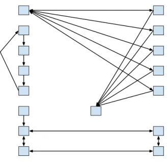
Actually, dedicated wires are required for each communication ﬂow, i.e., in some cases, two communicating nodes require two set of linking wires between them, one for sending data from the former node to the second node and another set for the opposite ﬂow. For instance, the number of bidirectional channels to connect all processing elements in an architecture with n processing elements is n×n−1.

Figure 2.2: Point-to-point infrastructure with sixteen processing elements. See that not every link direction is implemented.

Figure 2.2 shows a point-to-point architecture with sixteen processing elements. Note that not all channels are mandatory, actually, non-communicating processing elements do not need to have channels to interconnect them and there are channels with a single direction.

2.2.2 Bus

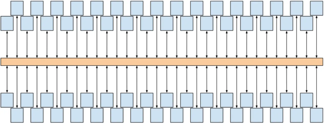
A bus is a set of wires that are shared between devices to connect them so they can transmit data to each other. Buses have important characteristics like the smaller complexity of implementation compared to point-to-point and also the eﬃcient use of wires, given that less wires are needed to connect processing elements.

(29)

29

Figure 2.3: Bus connecting 64 processing elements.

A common concept involved in buses implementation is arbitration. Arbitration is respon-sible for granting access to the bus following an access policy. Such policy is necessary to share the bus and also to avoid data corruption and starvation1 _{between bus members.}

The most used arbitration policies are round-robin arbitration and arbitration based on priorities. The former treats requests with the same priority and grant access based on a fair sequence. The second one respect a priority list to grant access to the bus. Still related to arbitration, there are more speciﬁc techniques like burst mode data transmission [LRD01], where the master negotiates with the arbiter to send multiple words of data over the bus without incurring the overhead of handshaking for each word.

Considering that buses share wires between several processing elements it is not possible to have multiples transmissions simultaneously. Actually, to reach such feature more elaborated techniques like hierarchical buses are needed.

The fact that it is not possible to have multiples transmissions simultaneously results in a very important drawback to buses. As more and more devices are attached to the bus, it becomes a bottleneck of the system. It happens because of the existence of contention to receive access to the media. Contention occurs when one or more elements are requesting access to the media but another element is transmitting through the media.

The fact that contention occurs when a bigger number of processing elements are attached to the media implies in low scalability. Scalability is the ability of systems to grow and handle the growth of work in such a way that there is no degradation of the requisites of the system. Nowadays this characteristics is becoming more important, that is why other network structures like Network-on-Chips became so relevant.

1_{Starvation occurs when a device requests access to a resource but the access is never granted though there is no}

(30)

30

2.2.3 Network-on-Chip

According to [BM06], there are two widely used perceptions of NoC. The former says that NoC is a subset of SoC, and second one that NoC is an extension of SoC. In the ﬁrst perspective NoCs is an alternative to the communication problem of intra-chip system and is basically referred as an physical media. On the other hand, the second perspective is more broadly concept and also encompass related issues that were noticed with the appearance of NoCs.

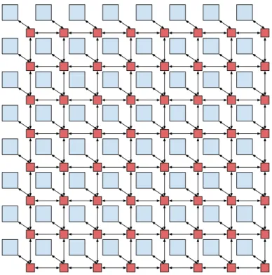
As said in Chapter 1, NoCs can be deﬁned as intra-chip communication subsystem, usually composed by a set of routers interconnected by point-to-point communication channels, implement-ing a chosen topology. One common example of topology used is the Mesh due to its regularity. Figure 2.4 shows a mesh-based network with 64 processing elements - 8 columns and 8 rows of elements. Routers are represented by red squares, while processing elements are represented by blue squares. Arrows indicates links between adjacent components.

Figure 2.4: 8x8 mesh-based NoC interconnecting 64 processing elements.

(31)

31

The arbitration problem, common to buses, also exists in the NoC but it has several diﬀerences. The arbiter, instead of arbitrate the access of elements to the shared wires, it is responsible for orchestrate how and the order in that adjacent routers forwards data through links. So, instead of a centralized point of arbitration, NoC distributes this problem between neighbour routers.

There are also new issues that were known in the broad sense of communication but were not previously seen in the field of intra-chip system. For example, concepts like circuit or packet switching, routing algorithms and connection-oriented and connectionless also need to be discussed by system designers. All these concepts were known issues in the broad research field of communication but are now also requiring designers attention in the field of intra-chip systems. Therefore, it is possible to say that in spite of the advantages of network-on-chips, this approach introduces complexity to the design of such systems. More details about these concepts are discussed in the following sections of volume.

Usually, network-on-chips are divided into three main components. Network interfaces, also known as network adapters, that implement the interface by which processing elements are connected to the rest of the network. Their function is to decouple computation from communication. Another component are the routers. They are in charge of routing data across the network. Such components can be implemented in many ways but they use to contain arbiters, buﬀers, crossbars and a hard-wired algorithm called routing algorithm. And, at last, links composed by channels are in charge of connecting routers to processing elements.

According to [GG00], NoCs have few advantages and disadvantages when compared to buses. Few of the main pros are:

1. Only point-to-point one-way wires are used, for all network sizes. It happens because each channel is composed by two links: one for input and another for output, thus, both of them can be used to forward diﬀerent packets without interfere each other.

2. The same router may be instantiated again, for all network sizes, what represents reusability to designs using NoCs.

3. Aggregated bandwidth scales with the network size, in opposite to bus.

4. The routing decision can be distributed, what makes fault-tolerant solutions possible. For instance, adaptive routing policies can handle spoiled tiles avoiding to forward packets through them.

The four advantages covered above represent respectively four known concepts to SoC design: a) parallelism; b) reusability; c) scalability; and d) reliability. These concepts add value to systems but there are also several drawbacks.

(32)

32

depending on where communicating tasks are placed, more or less hops are necessary to transmit messages. It reflects on other systems constraint like energy, heat and communication throughput. From the perspective of area, intra-chip networks are bigger because there are waiting FIFOs (buffer registers) and logic control segments for arbitration, crossbar and flit forwarding. Such registers and control segments would not exists or would at least be less complex in simpler architectures like buses. Finally, the adoption of network-on-chips requires a re-education of designers and developers in order to understand and better exploit the architecture’s potential.

2.2.4 Clustered NoC

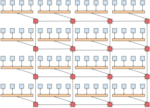
A clustered NoC is a special type of network that, instead of linking routers to processing elements, it links routers with a second topology. Some may say that clustered NoCs are multilevel architectures.

Figure 2.5: 4x4x4 mesh-based NoC.

(33)

33

Because of the fact that cluster-based architectures are hybrid solutions of bus and NoC, it is clear to assert that it is a more complex structure than NoC and bus separately. This characteristic obviously demands more attention and eﬀort from designers. Besides, designers have to avoid clusters with too many communicating nodes, since it may cause the same contention that exists in bus-based topologies.

So, this architecture was designed in such a way that it takes beneﬁts from both topologies, the low-cost usage presented in buses coupled with the NoC’s greater communication capability and ﬂexibility. It gives to the designer a greater possibility range to map the system elements over the architecture. Consequently, the new mapping possibilities open new design choices that enrich the design space exploration.

(34)

(35)

35

3. RELATED WORKS

This section is divided in three fields. The first one collects well-known approaches to mapping applications onto Network-on-Chips. Then, a more specific study is presented where only works related to mapping application onto cluster-based MPSoCs are shown. And then, a comparison of this work with the ones previously presented is made.

3.1 Mapping techniques for Network-on-Chip

There are many works that emphasize the importance and complexity of mapping and partitioning application tasks in NoCs. They started as soon as NoCs have arisen as a prominent alternative to design MPSoCs.

One of the most known works that explores the mapping of applications to NoCs ar-chitecture was made by Marculescu [HM03]. It captures the number of bit transitions based on an application characterization model, which is described by Marcon [Mar05] as communication-weighted model (CWM). CWM uses the communication-communication-weighted graph (CWG), a simple graph that exposes average communication loads between tasks. In spite of being a simple model, it has few disadvantages, like it cannot represent dependency and order between communications. In addition, it demands eﬀorts from designer to elaborate and label communication arrows with their loads. If arrows are not properly labelled, result precision is decreased from the mapping result.

In [MDM04], the authors present a heuristic algorithm to solve the mapping problem. The algorithm speciﬁcally explores bandwidth constraints of mesh NoCs. The objective is to minimize the average delay and it is validated by cycle-accurate simulation of a DSP design modelled in SystemC to which NoC components are added from the xpipes library. Their communication model is similar to the model shown in [HM03] and the heuristic algorithm has a behaviour divided into three steps: i) initial mapping generation, based on a maximum communication ordering of modules,ii) shortest path computation using Djikstra’s algorithm andiii) iterative improvement, by swapping pairs of modules and re-computing shortest paths. Another very simple explanation about the approach, is that it labels links with its utilization/load and it explores mappings whose paths between communicating nodes have smaller link loads. One interesting fact of that work, is that one of the activities listed as future work, is to extend the model to map cores onto various NoC topologies, enabling the NoC topology selection.

(36)

36

In [MMCM08], the authors collect results of a set of mapping algorithms to map appli-cations to NoCs. The types of algorithms explored comprehend approaches like exhaustive search, stochastic search methods, heuristics, and combinations of stochastic and heuristic algorithms. As input, a communication-weighted graph served as basis to produce a set of experiments representing communication patterns for various applications. The objective of that work is to explore low energy consumption mappings.

3.2 Mapping techniques for cluster-based MPSoCs

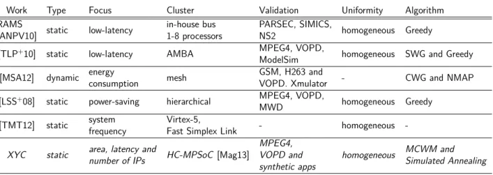
In this section, several works that emphasize the mapping of applications onto cluster-based MPSoCs are presented. At the end, Table 3.1 shows in a tabular manner their diﬀerences.

The authors from [ANPV10] contributed with a system that provides a multi-bus execution environment where each processor is connected to a bus and the bus-based subsystems communicate via routers connected in a mesh-style conﬁguration. They make a study to evaluate memory access patterns and this study indicates that while a hybrid architecture is preferable, the optimal number of processors on each bus subsystem varies based on the application. This number appears to vary between 1 and 8 depending on the communication requirements of the application. Therefore, they proposed having a reconﬁgurable interconnect, where the number of cores per bus is variable and assigned by the operating system at run time.

In [TLP+_{10], a bus-mesh hybrid architecture to provide a low latency communication}

environment for SoC Design was proposed. Their basic idea is to utilize the communication feature of each IP to decide the IP location. In the proposed hybrid architecture, the IPs with heavy traﬃc and communication aﬃnity are placed in the same bus-based subsystem to avoid hot-spots and reduce the transmission latency. Since the hybrid architecture is based on NoC concept, the router of the hybrid system not only connects with its neighbour routers but also connects to a single IP or a bus-based subsystem. It is noteworthy that a new interface is not needed for each IP in subsystem, and it can further reduce the design cost and power consumption. It also contributes with partitioning and mapping greedy algorithms that has as input the network dimensions and a communication graph.

In [MSA12] a work that explores reconfigurability was also presented. The authors proposed an architecture whose nodes are grouped into some clusters interconnected by a reconfigurable communication infrastructure. From the traffic management perspective, this structure benefits from the interesting characteristics of the mesh topology (efficient handling of local traffic where each node communicates with its neighbours), while avoids its drawbacks (the lack of short paths between remotely located nodes). The work uses few approaches presented by [MDM04] but proposed few adjusts, so that, the existing algorithms could be used with the proposed architecture organization.

In [LSS+_{08], the authors proposed a hierarchical cluster-based customization method. It’s}

(37)

37

another one for hierarchically compose and organize the network infrastructure and a third one to remove unused network links. This approach is very application speciﬁc and its partitioning algorithm has as input a communication-weighted graph, what opens possibilities to improvements with a communication graph that brings more characteristics about communications.

In [TMT12], an indicator based on average Rent’s Rule [CS00] was proposed to map applications to cluster-based MPSoCs. The objective is to predict the best form factor of MPSoCs to obtain the maximum system frequency for a given multi-FPGA prototyping platform and a given number of processing elements. To accomplish that, a generic cluster-based MPSoC, based on the Xilinx Microblaze general purpose soft processor, was speciﬁcally designed. They build the platform in a manner that the number of clusters and the number of processing elements per cluster is generic. Another characteristic of it, is that both the cluster and the processing elements are all homogeneous. At the end, the target prototyping platform was performed using a six Virtex-5 FPGA board. In a more simple manner, they parametrize their network in three variables: X for NoC width, Y for NoC height and Z for the number of processing elements attached to each NoC tile. Then, they studied the inﬂuence of the form factor (X, Y and Z) in the system frequency when prototyping and based on this study they choose the best form factor.

Table 3.1: Comparison of cluster-based works.

Work Type Focus Cluster Validation Uniformity Algorithm

RAMS

[ANPV10] static low-latency

in-house bus 1-8 processors

PARSEC, SIMICS,

NS2 homogeneous Greedy

[TLP+_10] _static _low-latency _AMBA MPEG4, VOPD,

ModelSim homogeneous SWG and Greedy

[MSA12] dynamic energy

consumption mesh

GSM, H263 and

VOPD. Xmulator - CWG and NMAP

[LSS+_08] _static _power-saving _hierarchical MPEG4, VOPD,

MWD homogeneous Greedy

[TMT12] static system

frequency

Virtex-5,

Fast Simplex Link - homogeneous

-XYC static area, latency and

number of IPs HC-MPSoC [Mag13]

MPEG4, VOPD and synthetic apps

homogeneous MCWM and

Simulated Annealing

3.3 Distinction of Proposed Work

All the works presented in this section are related to cluster-based MPSoCs. They also have components known as routers that are in charge of composing the global communication infrastructure. However, our work has a strong distinction from the works [LSS+_{08] and [MSA12]}

because they do not use buses to implement their clusters, instead, they adopt hierarchical and mesh-based approaches, respectively.

The work being presented here does have aﬃnity with the works [ANPV10] and [TLP+_10],

(38)

38

but they may fall in very inefficient mappings when the set of inputs is not well defined. In addition to that, the CWG is a graph that characterizes communications as arrows, and each one is labelled with a load, that exposes the amount of data being transferred. Some may consider this approach too simple for the complex systems that are being designed nowadays. Therefore, a map tool that considers more variables is presented. In this map tool different architectures like bus, NoC and clustered-NoC are implemented and a comparison of their performance related to minimum latency is shown.

So, a mapping algorithm that uses a diﬀerent approach and a communication graph that describes more details about its contents were chosen. The approach adopted is the Simulated Annealing and the communication graph is presented in Section 4. The distinction of this work with the previously presented can be seen at the last line of Table 3.1.

(39)

39

4. PROPOSED WORK

The proposed flow is divided into three main logic steps. These steps work with models at different levels of data abstraction, but based on well defined structures it is possible to adapt the data from one step to another automatically. These steps are:

Simulation

Simulation is one of the most important steps since it generates a very sensitive model that will be the basis for the partition step. User will input its tasks and based on a simulation, each message transferred will be recorded. The record of each message will be used to compose the communication model.

Mapping

Optimization algorithms are applied to speciﬁc communication task graphs and architectures. The objective is to obtain mapping alternatives to delegate tasks to PEs. These candidates are constructed based on iterative methods that explore the solution space based on a cost function speciﬁed by the designer.

End-Source Generation and Target Simulation

With the support of source-code adaptors, simulators and prototype builders, the designer has tools to validate the obtained mapping candidate.

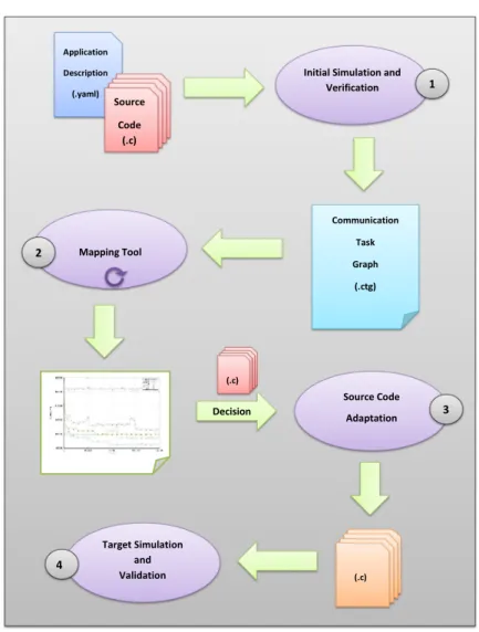
An overview of the whole ﬂow is presented in Figure 4.1. The arrows and the sheets represent respectively dependency of stages and artefacts. These artefacts can be both input and output to other steps. The content syntax of each artefact is explicit in the brackets. Circles are visual representation of automated tools of the proposed ﬂow.

The implemented work can be divided into three groups of software. The former group is responsible for the mapping step. All the models and decisions related to that subject are explained in Section 4.1. The second group of software is related to the Hellfire System. Actually it extends or modifies the Hellfire System in specific points and the work done in this field is presented in Section 4.2. The last group of the tools is a set of independent programs that implements the work flow proposed as the novelty of this work (circles of the Figure 4.1). These programs compose the XYC Toolchain and are presented in Section 4.3.

(40)

40 Application Description (.yaml) Source Code (.c)

Initial Simulation and Verification Communication Task Graph (.ctg) Mapping Tool Decision Source Code Adaptation Target Simulation and Validation (.c) (.c) 1 2 3 4

Figure 4.1: Flow to map applications to target architectures.

4.1 Adopted Models and the Mapping Step

There are several parts and decisions needed to implement the mapping step of the work ﬂow. For instance, it is necessary to specify the input, and chose the target architectures, so, these activities are explained in Sections 4.1.1 and 4.1.2. Additionally, algorithms and function costs are needed, so, Section 4.1.3 exposes the function cost adopted while Section 4.1.4 shows the implemented mapping algorithms.

4.1.1 Communication Task Graphs

(41)

41

Definition 1: A communication-weighted graph is a directed graph, G(Γ,E), where each vertexs ∈Γrepresents a task implemented to a deﬁned processor and labelled with a cpu utilization 0<us ≤1. The directed edge s →d(d ∈Γ) denotes the communication ﬂow from task s to task d. Each edge s →d is labelled with vsd, the average volume of communication between s and d is

represented in bits.

Definition 2: The modifed communication-weighted graph is a directed graph, G(Γ,E), where each vertex s ∈ Γ represents a task implemented to a deﬁned processor and labelled with a cpu utilization 0<us ≤1. The directed edges →d(d ∈Γ) denotes the communication ﬂow from

task s to task d. Each edge s → d has two attributes, denoted by vsd and fsd, where vsd is the

average volume of communication betweens and d, while 0<fsd ≤1 means the average frequency

of packets designated to d and injected by s into the communication structure.

CWM takes only into consideration the amount of transmitted data and it does not consider the channel occupation. On the other hand, MCWM tries to explore this characteristic with the f

attribute assigned to every communication edge. The choice of a good value forf must be carefully done, once it will play an important role on the results of the experiments and might vary a lot according to diﬀerent task mappings. As previously mentioned, MCWM is a superset of CWM. So, if every f attribute of the MCWM is assigned with the value 1, then the resulting mapping cost is the same to the equivalent CWM. So, when this information is available, the designer can obtain better estimations, if not, it is still possible to use it according to the widely adopted model.

4.1.2 Abstract Architectures

Based on three basic components it is possible to conﬁgure many architectures and compare them using the same metric. These three components are Routers, Processors and Channels. The implemented architectures are Bus, NoC and cluster-based NoC. See that these architectures are high-level representations and are not related to resembling components implemented in Section 4.2.1.

(42)

42

(a) Bus

(b) 4×4 NoC (c) 2×2×4 cluster-based NoC

Figure 4.2: Diﬀerent topologies composed by Routers, Processors and Channels.

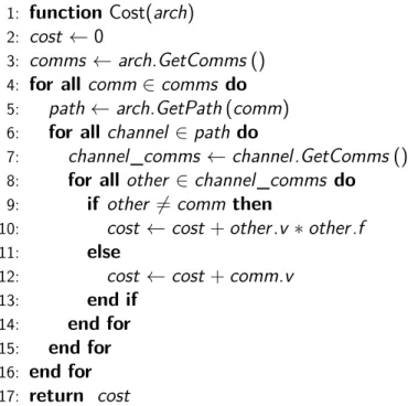
4.1.3 Function Cost

Depending on the cost function that designers use, diﬀerent aspects of the application can be evaluated. Most of the aspects evaluated taken into consideration are energy, heat dissipation or latency. Each of them can be better evaluated depending on the available data informed because the eﬃciency of each cost function depends both on the characterization of the communication model as well as on the target architecture. The cost function adopted in this work focuses on latency and it is based on the models described in previous sections. Its implementation is described in Figure 4.3.

The arch parameter is a high-level representation of the architecture that considers that tasks are already mapped to speciﬁc processors of the architecture. The tasks are mapped to processors according to a scheduling policy. Three policies have being implemented in this work: (1) best eﬀort, (2) rate monotonic and a (3) hybrid one. The arch parameter has the method

GetComms() that returns a set of communications edges (comms) of the communication graph. Thearch parameter has also a method that given a speciﬁc communication edge, it returns a set of

(43)

43

1: functionCost(arch)

2: cost ←0

3: comms ←arch.GetComms() 4: for all comm ∈comms do 5: path ←arch.GetPath(comm)

6: for all channel ∈path do

7: channel_comms ←channel.GetComms()

8: for all other ∈channel_comms do 9: if other 6=comm then

10: cost ←cost+other.v ∗other.f

11: else

12: cost ←cost+comm.v

13: end if

14: end for 15: end for 16: end for 17: return cost

Figure 4.3: Description of the cost function.

called GetComms(), but in that case, the method returns all comms that pass through the speciﬁc

channel before being delivered to the message destination. With this information it is possible to obtain the costs to send messages in every single channel and sum these costs to obtain an estimation ofarch’s mapping quality.

The meaning of the returned cost represents the number of bits (in the worst case) necessary to be forwarded before a message can be delivered. Considering that the objective function is implementing a worst case approach, the absolute value returned should not be taken as a meaningful value. However, when using the same metric with other architecture models, it is possible to use the cost variation to evaluate the architectures and consequently take a decision based on that diﬀerence. In other terms, this technique calculates the mapping cost and bigger values mean that more obstructed are the channels involved in the transmission of the messages. This technique is also known as PathLoad exploration.

4.1.4 Mapping Algorithms

(44)

44

it is possible to develop other algorithms. These implementations are based on two basic algorithms and their variations. The algorithms are Random Algorithm and Simulated Annealing, and their characteristics are detailed below.

Random Algorithm

The random approach is a primitive algorithm that is not usually adopted since it is possi-ble to obtain better results with other techniques. However, it serves as basis for many optimization algorithms, including Simulated Annealing. Even though this technique is rarely adopted, the algo-rithm was implemented in order to obtain a baseline for comparisons. The algoalgo-rithm is illustrated in Figure 4.4.

1: functionRandom(arch)

2: best ←RandomMapping(arch)

3: best_cost ←Cost(best)

4: whilestop_condition do

5: alternative ←RandomMapping(arch)

6: alternative_cost ←Cost(alternative)

7: if alternative_cost ≤best_cost then 8: best ←alternative

9: best_cost ←alternative_cost 10: end if

11: end while

Figure 4.4: Random mapping algorithm.

Simulated Annealing

Simulated Annealing (SA) is a generic probabilistic meta-algorithm for global optimization problems, namely locating a good approximation to the global optimum of a given function in a large search space [KGV83]. The technique was developed in 1983 and forms the basis of an optimization technique for combinatorial and other problems. It is widely used in a large range of applications and is inspired by the annealing technique in metallurgy. This technique involves heating and controlled cooling a material to increase the size of its crystals and reduce their defects. The heat causes the atoms to become unstuck from their initial position and wander randomly through states of higher energy.

In spite of the fact that Simulated Annealing is a widely adopted algorithm, there are emerging technologies like clustered-NoCs that were not yet addressed by this approach. With that in mind, this work focuses on the study of three implementations of the Simulated Annealing that handles the tasks mapping issue in clustered architectures.

(45)

45

some iterations, the algorithm may accept changes of the best known solution for another one that increases the cost function (assuming it is a minimization problem). These changes that increase the cost are accepted according to a probabilityp = exp(∆c÷T), where∆c denotes the increase of the cost function and T is a control variable. At every iteration the variableT (popularly known as temperature) decreases, and consequently, the probability of not accepting bad mappings candidates increases.

The implementation of the Simulated Annealing can be seen in Figure 4.5. There is another detail that differs SA from the random algorithm beyond the mechanism to accept or not a new solution. On line 5, the method Copy() copies the whole best known solution. Later, on line 6, it applies a modification using method Modify(). This method changes the location of a single task and calculates the mapping costs again. So, unlike the random algorithm which generates a completely different mapping at each iteration, the implementation of the Simulated Annealing only performs a modification in an architecture representation that is a copy of the momentary best mapping.

1: functionSimulatedAnnealing(arch)

2: best ←InitialMapping(arch) 3: best_cost ←Cost(best)

4: whilestop_condition do 5: alternative ←Copy(best)

6: alternative ←Modify(alternative)

7: alternative_cost ←Cost(alternative)

8: ∆←best_cost−alternative_cost

9: if exp(∆÷temperature)≥Random()then 10: best ←alternative

13: temperature ←temperature×α 14: end while

Figure 4.5: Traditional implementation of the Simulated Annealing.

Nested Simulated Annealing

(46)

46

1: functionNestedSimulatedAnnealingV1(arch)

2: best ←InitialMapping(arch)

4: whileouter_stop_condition do 5: alternative ←Copy(best)

6: alternative ←ModifySubstantially(alternative) 7: while inner_stop_condition do

8: alternative ←ModifySlightly (alternative) 9: alternative_cost ←Cost(alternative)

10: _∆←best_cost−alternative_cost

11: if exp(∆÷temperature)≥Random() then 12: best ←Copy(alternative)

15: temperature ←temperature×α 16: end while

17: end while

Figure 4.6: Second implementation of the Simulated Annealing.

1: functionNestedSimulatedAnnealingV2(arch) 2: best ←InitialMapping(arch)

4: whileouter_stop_condition do 5: list ←[]

6: while inner_stop_condition do 7: alternative ←Copy(best)

8: alternative ←Modify(alternative)

9: alternative_cost ←Cost(alternative) 10: list ←list+ [(alternative,alternative_cost)] 11: temperature ←temperature×α

12: end while

13: alternative,alternative_cost ←Min(list)

14: _∆←best_cost−alternative_cost

15: if exp(∆÷temperature)≥Random()then

16: best ←Copy(alternative)

19: end while

(47)

47

The implementation of the Nested Simulated Annealing is shown in Figure 4.6. This imple-mentation has two different methods: ModifySubstantially() and ModifySlightly(). Both methods are called with tasks already mapped to the architecture. The first method changes the position of ⌈t ÷2⌉ tasks of the architecture, given that t is the total number of tasks. We consider that changing the position of ⌈t ÷2⌉ tasks is a substantial modification because half of the tasks are moved. The later method does the migration of one task and is equivalent to the method Modify() from the previous implementation.

Figure 4.7 describes the implementation of a second variant of the Nested Simulated Annealing. The cost functions calculated in the inner loop and the modiﬁcation performed by the Modify() method are stored in a list sequentially. After each iteration of the outer loop, the best

move stored on the list is chosen as the new candidate to be tested in the acceptance test. The method Min() returns respectively the architecture with a mapping description and its cost. The variable inner_stop_condition is a simple controller that iterates ⌈t÷2⌉ times.

4.2 Hellfire System

The Hellﬁre System is a set of subsystems and modules. These modules are basically tools that support designers to build embedded systems. Between the group of main modules we can mention the following:

Hellfire OS

Embedded realtime operating system.

Hardware Modules

Set of modules as processor, bus, NoC and Clustered NoC described in HDL.

MPSim

Simulator that emulates all hardware modules.

Web-Framework

An online Integrated Development Environment.

The most important of the modules probably is the HellfireOS (HFOS). It is a real-time operating system (RTOS) developed intending to ensure maximum flexibility on its configuration and allow a high-level platform customization. In order to allow such features, the HFOS was implemented in a modular way, where each module corresponds to some specific functionality.

(48)

48

implementation, the HellﬁreOS is easily portable to others architectures, requiring only the rewrite of hardware-dependent functions, implemented in the HAL.

In order to decrease the kernel final size, allowing HFOS to be used even in architectures with severe memory limitations, parameters such as maximum number of user tasks, stack and heap size and drivers are configurable. The user applications are written using the C programming language and the HellfireOS API.

All the architectures implemented and the drivers are focused to run with or over Hellﬁre OS. Based on that, the implemented communication medias are presented below and after that an explanation of the communication driver is also given.

4.2.1 Implemented Architectures

Architecture like Bus, NoC and CNoC are already implemented in the Hellﬁre System but they were described using a hardware description language [AFM+_{10]. Not all architectures were}

represented in high-level languages in such a way that it is possible to run fast simulations with them. Due to that, high-level implementations of the existing architectures (Bus and NoC) were reviewed and the behaviour of the clustered NoC was implemented in C language.

The implementation of these three architectures have relevant distinctions and they are described below. In addition to that, some components common to the three architectures are also presented.

Common Concepts

There are some concepts that are common and presented in the three studied architectures. They are Network Interfaces, Flits, Packets, Message and Memory Mapped Addresses.

Messages are data sent between communicating tasks. The message before being injected into the communication media is divided into packets. Packets can have fixed or flexible size but in this work fixed-sized packets were chosen.

Packets are composed by smaller parts, the flits. Flits represent the smallest amount of data meaningful for the communication media. Usually flits can have two classification: header flits and payload flits. Header flits are meaningful for the communication media because they specify useful information for the forwarding of the following packet’s flits. On the other hand, payload flits are irrelevant data for the communication media, i.e., they only have to be passed on.

(49)

49

NIs are composed by two FIFOs. One of the FIFOs is responsible for storing data injected from attached devices and for forwarding data to the network media. The other FIFO is responsible for the opposite data ﬂow. It stores data from communication media and forwards the data to the attached devices.

Bus

Figure 4.8 shows the block diagram of the bus speciﬁcation. The bus is composed by parametrizable network interfaces and a logic control that handles arbitration and ﬂits forwarding. The blue squares are the attached devices. In particular, this work allows only processors to be attached to the bus. The main advantage of this architecture is the resulting area that is smaller than the next architectures because it has a single simple module, the own bus.

CPU Node

Forward and arbiter logic

CPU

Node NodeCPU NodeCPU

Network interface buffers

...

Memory mapped registers

Figure 4.8: Bus speciﬁcation.

Network-on-Chip

For our NoC implementation we use HERMES NoC [MCM+_{04], which implements a mesh}

topology and is composed by routers, buffers and controllers of routers information (switch control). HERMES routers can have up to five operating channels. Channels are composed by buffers fed by incoming and outgoing ports. Ports are wires that connect adjacent routers.

As mentioned above, routers can have from two to ﬁve channels because routers allocated in the border of mesh do not have all adjacent routers, thus, the respective channels are unnecessary. Moreover, not every router need to be attached to a processing element by the port known as local port. In such situations these channels are unnecessary too.

An overview of the NoC Router is shown in Figure 4.9. Blue squares represent the devices attached to the media while red components are the parts that compose communication media. Please, pay attention the fact that each router has one buffer for each port. It was made like that because outgoing flits go directly to the router adjacent incoming buffer.

(50)

50 ... ... CPU Node Memory mapped registers Network Interface Buffers Routing and arbiter logic Channel buffers Neighbor input buffer

Figure 4.9: Router speciﬁcation.

the control flow strategy, the buffers’ size and the arbiter policy. This work uses the XY routing algorithm since it is a simple and deadlock free algorithm. This work uses rotative arbiter due to the fact that it does not suffer from starvation and also because it’s algorithm is not complex. Finally, this work chose handshake as the control flow strategy because in the future the Hellfire Systems will enable heterogeneous mixed architecture and such control strategy is favourable to this reason.

Clustered Network-on-Chip

The implementation of the high-level clustered NoC respects precisely the behaviour of the CNoC implemented by GSE [Mag13]. In addition to that, they use identical routers as the NoC speciﬁcation.

However, unlike NoC, clustered NoC does not link network interfaces to routers’ local port buffers. Instead of that the local port buffers are linked to another module called cluster interface (CI). CI is a module with the same behaviour as network interface but it is an intermediate step to forward packets from bus to NoC routers and vice versa. In Figure 4.10 it is possible to see how bus and NoC router are linked by the cluster interface and the local port buffer.

4.2.2 Communication Driver

The communication protocol was implemented as a Hellfire OS driver. Therefore, it is possible to evaluate different communicating applications using the tools available by the Hellfire Web-Framework.

(51)

51 Forward and arbiter logic input buffer CPU Node

Forward and arbiter logic

Cluster interface buffers

CPU

Node NodeCPU NodeCPU

Network interface buffers

...

Memory mapped registers

Neighbor input buffer

Figure 4.10: CNoC Local Interface Structure.

below application layer is the Transport Layer. This layer basically split messages into packets and reassemble messages. It is also responsible for handling unordered packets or messages whose time-outs were reached. After that, lies the Network Layer. The network layer adds or removes the header required by the communication media. We will see that diﬀerent media require diﬀerent headers. Finally, the last layer is the Link Layer. This last layer basically interacts with Networks Interfaces through memory mapped addresses.

Table 4.1: Hellﬁre communication primitives.

Signature

uint32 HF_NB_Send(uint16_t target_cpu, uint8_t target_id, uint8_t buf[], uint16_t size, uint32_t timeout) uint32 HF_Send(uint16_t target_cpu, uint8_t target_id, uint8_t buf[], uint16_t size)

uint32 HF_NB_Receive(uint16_t *source_cpu, uint8_t *source_id, uint8_t buf[], uint16_t *size, uint32_t timeout) uint32 HF_Receive(uint16_t *source_cpu, uint8_t *source_id, uint8_t buf[], uint16_t *size)

(52)

52

Finally, the NET_WRITE register is used to insert ﬂits to the network interface and should be called after a polling process on the NET_STATUS register.

TARGET

0 15

PAYLOAD

16 31

SOURCE CPU ID

32 47 SOUR. TASK 48 63 MESSAGE SIZE 64 79 PACKET SEQUENCE 80 95

CONTROL FLOW FLAG

96 111

CRC

112 127

DEST. TASK

Figure 4.11: Communication protocol header.

Figure 4.11 shows the communication protocol header. Flit target and ﬂit payload compose the header required by the media. Target varies with the media, but payload has the same meaning in every architecture and means how many ﬂits are remaining in the body of a packet.

SOURCE CPU ID is a decimal ﬁeld that answers what was the processing element that injected the packet into the network. This data is useful for the application layer since it is possible to identify in run-time the sender of the received messages.

SOURCE TASK and DESTINATION TASK are useful for the transport layer. With this data, it is possible to address messages to nodes running more than one task, for instance, nodes running operating systems and their applications. Other ﬂits important for the transport layer are MESSAGE SIZE and PACKET SEQUENCE. They are complementary data and they are used by transport layer on the reassembling message process.

Other optional data of the header are CONTROL FLOW FLAG (CFF) and CRC. CFF is a ﬂag that tells driver if an packet received should generate an acknowledge message. CRC is an abbreviation Cyclic Redundancy Check and is used to check whether any data corruption occurred.

Figure 4.12 shows how the TARGET flit differs from one communication media to another. At that point it is important to remember that although Hellfire System tools enable different sizes for the flit, this work adopts flits with 16 bits as its default flit size. Actually, bigger sizes can be chosen but smaller sizes would not fit with cluster-based architectures.

The bus target flit is the simplest one. It basically uses the eight least significant bits to indicate the target CPU. It means that 256 processing elements can be attached to the bus, though we do not encourage the use of bus with such amount of elements. The remaining most significant bits are unused.

(53)

53

0 15

TARGET ID

COL ID LINE ID

COL ID LINE ID CLU ID

BUS DESTINATION FLIT

NOC DESTINATION FLIT

CNOC DESTINATION FLIT

Figure 4.12: Target ﬂit speciﬁcation.

the y-axis target position. Considering that COL ID and LINE ID are four bits ﬁelds, it is possible to build NoCs with 256 tiles (16×16).

As it was already explained, cluster-based NoCs are clusters connected by network routers. Considering that the networks are all implemented using the mesh topology, we say that COL ID and LINE ID identifies target cluster ID on x-axis and y-axis respectively. In addition to these fields, there is still the cluster position ID field. It is useful to identify the CPU position inside each cluster. Considering that the three fields are 4 bits each, it is possible to build CNoC architectures with 256 clusters and each cluster can support up to sixteen processing elements. The remaining most significant bits are unused.

4.3 XYC Toolchain

At that point we present the set of tools that implement the proposed work ﬂow. See Section 4 for more details about that ﬂow. Pay attention to the fact that the output of the each tool serves as input for the next tool on the software chain.

4.3.1 XYCSIM - XYC Simulator

XYCSIM is essentially a platform generator. The platform obtained using the tool can be simulated using OVP [OVP12], a virtual platform simulator, or even using the simulators imple-mented in GSE. The objective of this simulation is to obtain a MCWG. The MCWG is used as input by the next tool, the XYCMAP.

(54)

54

task of the task set. There are two mandatory inputs: -tasks and -procs. -tasksis a string parameter that points to a ﬁle that contains a list of tasks. -procsis a string parameter too but it points to a ﬁle that list processors and describes their characteristics. Figure 4.13 shows tool’s interface.

Figure 4.13: XYCSIM help command.

4.3.2 XYCMAP - XYC Mapper

Figure 4.14 shows the text-based user interface of the tool. The ﬁgure shows the range of parameters available. The most important parameters are the -arch, -x, -y, -c, -b,

-input, -output, -policy, and -algorithm. The -input parameter is a name to

(55)

55

Figure 4.14: XYCMAP help command.

Considering that the parameters -x, -y, -c, and -b are set of lists results in an important effect on the mapping phase. It makes the mapping process aggressively more time consuming because of the growth caused by the combination of acceptable configuration. To mitigate this growth of the explorable space a simple policy was used. Once an arrangement that respects the scheduling policy is found, no new arrangements can use more processing elements than that one. This simple alternative is enough to prevent the algorithm from testing too consuming arrangements, while easily covers simple decisions that designers have to take, like choosing square architectures, or irregular ones, like rectangular or even pipelined ones. Alternatively, the designer can input single values for each axis, then the mapping algorithm is applied to a single architecture configuration. See that this feature is one of the goals of the work, once it explores architectures with smallest number of processing elements.

The-policyparameter deﬁnes guard for accepted tasks arrangements. At each iteration of the mapping tool a new task arrangement is obtained. This arrangement is tested against a scheduling policy. If the test does not succeed, the arrangement is discarded. Currently, only Rate Monotonic (RM) and Best Eﬀort (BE) were implemented, but it is possible to implement other policies like single task execution per node or other real-time scheduling algorithms.

The last important parameter is -algorithm. It deﬁnes the mapping algorithm that should be used to map tasks to processors. Currently, there are four algorithms implemented but it is possible to add new ones. The ones implemented were presented in the previous sections of this document.

(56)

56

4.3.3 XYCADAPT - XYC Adaptor

The third tool of the toolchain performs a important task of the proposed flow. It takes ANSI C tasks and converts them to Hellfire OS tasks based on a mapping file. To ease the trans-formation the ANSI C tasks requires some annotations using comments.

The parameters -tasks and -procs are string parameters that points to two distinct files, one that contain a list of tasks and their attributes, and the other a list of processors and their characteristics. The other parameter that is the most important is the-map file. This file contains a mapping arrangement that specifies a network communication infrastructure and also defines the location of each task (from -tasks parameter) to a tile of the network. Figure 4.15 shows the tool’s interface.

Figure 4.15: XYCADAPT help command.

4.3.4 XYCPRO - XYC Prototype builder

Finally, the last tool of the XYC toolchain is responsible for building a runnable instance of the architecture. Actually the target architecture depends directly on the mapping parameters given to the XYCMAP tool. The architectures available are those shown in Section 4.2.1.

Similarly to the XYCSIM tool, the XYCPRO is also a union of three other smaller builders. One tool is responsible for creating a makefile that will be used to compile the platform and operating system binary objects. The second builder creates an OVP platform model. The last builder creates a C header file that identifies tasks. This header file is especially important because it provides information to properly address packets given that packet header varies depending on the chosen architecture. See Section 4.2.2 for more details about it.

(57)

57

(58)