Phase transition of demand explained by the heterogeneity of
consumers’ intrinsic preferences
Fernando Pigeard de A. Prado,1 Vladimir Belitsky
Institute of Mathematics and Statistics, University of S˜ao Paulo, Brazil
Paolo Tommasini
Presidente de Moraes College, S˜ao Paulo, Brazil
Abstract
In 1991 Gary S. Becker presented A Note on Restaurant Pricing and Other Examples of Social Influences on Price explaining why many successful restaurants, plays, sporting events, and other activities do not raise their prices even with persistent excess demand. The main reason for this is due to the discontinuity of stable demands, which is explained in Becker’s (1991) analysis.
In the present paper we construct a discrete time stochastic model of socially in-teracting consumers deciding for one of two establishments. With this model we show that the discontinuity of stable demands, proposed by Gary S. Becker, depends crucially on an additional factor: the dispersion of the consumers’ intrinsic preferences for the establishments.
Keywords: Heterogeneity of consumers’ preferences, social interactions, social influence on price, discontinuity of demand, multiple demand equilibria.
JEL Classification codes: D11, D4, M30
1The corresponding author. Instituto de Matem´atica e Estat´ıstica, Universidade de S˜ao Paulo,
Phase transition of demand explained by the heterogeneity of
consumers’ intrinsic preferences
1
Introduction
As explained by Gary S. Becker (1991) in A Note on Restaurant Pricing and Other Examples of Social Influences on Price, the individual demands for establishments like restaurants, bars, night clubs, etc. are usually increasing functions of their aggregate demands. From this fact, Becker deduces that the resulting equilibrium demand which emerges in such cases, i.e., when the demand is positively auto-correlated, may appear to be discontinuous. This would explain why, for example, some restaurants do not raise price even when a given excess demand persists.
His explanation is essentially the following: if the demand is a continuous function of price, an over demanded restaurant could gradually raise prices in order to reduce its queue and increase profits without losing effective sales. On the other hand, supposing the existence of social interaction among consumers., a slight increase in prices could reduce not only the queue, but also the number of consumers who visit the restaurant motivated by the fact that the restaurant is over demanded. The resulting effect is that a slight increase in prices may reduce significantly (discontinuously) the restaurant’s demand, bringing it below the restaurant’s capacity and also below the profit maximizing sales level. This would explain the puzzle proposed by Gary S. Becker.
We claim that in addition to the social interaction among consumers, there is another factor that is crucial in determining when and why the demand for such establishments appears to be discontinuous in price. Namely, we show that if the consumers are suffi-ciently heterogeneous in their intrinsic preferences for establishments then the demand function is no longer discontinuous. Contrary to this case, that is, if consumers are rela-tively homogeneous in their intrinsic preferences, then the aggregate demand appears to be a discontinuous function of price.
The intrinsic preference of a consumer is defined in our model as the difference in prices between two establishments (or two distinct consumption options) for which this consumer is indifferent to the choice between them, when both establishments have the same level of aggregate demand, i.e., when both establishments are equally attractive from a social point of view.
in respect to their prices (this would explain why the over demanded restaurant does not raise prices, item ii)). Now, starting from our model, if we consider twosimilar (in an ex-treme case, identical) establishments competing for consumers in a market duopoly, then it is natural to suppose that all potential consumers of both establishments are relatively indifferent to the establishments, when both have the same level of aggregate demand. Therefore, when establishments are similar, it is also natural to suppose that the con-sumers are relatively homogeneous in their intrinsic preferences for establishments (all consumers have intrinsic preferences for the establishments close to zero). From this fact and also from the social interaction among consumers we would also deduce a concentra-tion of the resulting aggregate demand on one of two restaurants, and that the aggregate demands of both restaurants are discontinuous in respect to their prices.
We propose now to extend this analysis to the case when the restaurants offer dif-ferent services and amenities and/or when they are not located closely to one another, i.e., when they represent different consumption options for consumers, even when both establishments are equally demanded. Note that in this case, i.e., when the establish-ments are dissimilar, the consumers may have quite different intrinsic preferences for the establishments. This is illustrated by the example below.
Imagine a duopoly consisting of two competing night clubes in a rural area where there are no other night life options. Suppose also that these night clubes are similar in their services and amenities, but located relatively far way from each other. In this example, the intrinsic preference of a consumer is the difference in prices between the two night clubes that would compensate for the difference in the distance between each night club and the consumer’s house, when both night clubs are equally demanded. If all the potential consumers of both night clubs live in the same small village (it does not matter where in this rural area), then the dispersion of the consumers’ intrinsic preferences is relatively low. On the other hand, when their homes are uniformly distributed over this rural area, then the dispersion of the consumers’ intrinsic preferences for the night clubs is relatively high. According to our model, in this case, the dispersion of the differences of the distances between each night club and each consumers’s home will play a crucial role in determining when and why the aggregate demand appears to be concentrated on one of the night clubs and when and why the demands appear to be discontinuous in the night clubs’ prices.
2
The model
We model the situation where two establishments E(+) and E(−), say, two fashionable
night clubs, are competing for consumers in a market duopoly.
Let us denote the set of all potential consumers of both establishments by C :=
{1,2, . . . ,|C|}. We assume that at each time t= 0,1,2, . . ., say, weekends, N consumers selected from C, N ≤ |C|, decide for one of two establishments2. We shall denote by
Ct(N,C) the set of consumers selected at time t. For example, if |C|= 100, N = 3 and the
consumers 5, 20 and 99 are selected at time 1 thenC1(3,C) ={5; 20; 99}. The selection rule may be quite general but must be independent of the consumers’ intrinsic preferences. This independence will be formalized later in (8), after we have defined the intrinsic preferences of consumers.
Let us denote the number of consumers that choose establishment E(+) and E(−) at
timetbyNt(+1) andNt(−1), respectively (Nt(+1)+Nt(−1) =N,∀t). Let us also assume
that all potential consumers of both establishments (all elements of C) are aware of the popularity of both establishments in the recent past. In order to reflect this in our model, we assume that at each timet >0, each consumeri∈C knows the values of the fractions
Nt−1(+1)/N and Nt−1(−1)/N, where the values of N0(+1)/N and N0(−1)/N, i.e., the
initial demand fractions of the establishmentsE(+1) andE(−1), are two real numbers from
the interval [0,1], totaling one, that are independent ofN.
Let us now present the preference structure of the consumers. Fort≥1 andi∈Ct(N,C),
let us denote by Ut(i)(d) the utility of the consumer i in taking decision d ∈ {+1,−1} at
time t, i.e., in choosing the establishment E(d) at timet and queueing, if necessary (here
and from now on,E(+1):=E(+) and E(−1) :=E(−)).
To focus our attention on the main phenomena we are going to explain, we propose the following utility functions:
Ut(i)(d) :=J Nt−1(d)
N −p(d) +u
(i)(d),
∀t∈ {1,2, . . .}, ∀i∈Ct(N,C), ∀d∈ {−1,+1},
(1)
where J, p(d) and u(ti) are explained below.
J is a positive parameter, which measures the level of social influence on the utilities of consumers. This interpretation ofJ is clear from the fact thatNt−1(d)/N expresses
the popularity of the establishment E(d) (d ∈ {+1,−1}, t ≥ 0) in the immediate
past. The assumption of the positivity ofJ follows Becker’s (1991) explanation that assumes that “...a consumer’s demand for some good depends (positively) on the demands by other consumers. The motivation for this approach is the recognition that restaurant eating, watching a game or play, attending a concert, or talking about books are all social activities in which people consume a product or service together and partly in public.”
p(d) is positive and denotes the price charged by the establishmentE(d) (d∈ {+1,−1}).
u(i)(d)∈R is a consumer’s ispecific utility increment in choosing establishment E(d) at
time t (i∈Ct(N,C), d∈ {+1,−1}, t≥0).
For t ≥1 and i∈Ct(N,C), let us denote by d
(i)
t ∈ {+1,−1} the decision of consumer i
at time t; that is, if d(ti) = +1 (−1) then the consumeri goes to establishment E(+) (E(−)
respectively) (and queues if necessary). The utility maximization behavior implies that
Ut(i)(+1)−U
(i)
t (−1)>0 ⇒ d
(i)
t = +1
Ut(i)(+1)−U
(i)
t (−1)<0 ⇒ d
(i)
t =−1
(2)
To proceed, we need to define the consumer’s decision when Ut(i)(+1)−U
(i)
t (−1) = 0.
We assume that
Ut(i)(+1)−U
(i)
t (−1) = 0 ⇒ d
(i)
t =−1 (3)
As we will see, the assumption (3) does not cause an asymmetry in the resulting aggre-gate demand, since in accordance with the further descriptions of the model, the event
{Ut(i)(+1)−U
(i)
t (−1) = 0 for some i∈C
(N,C)
t } occurs with probability zero.
Now, from the utility functions defined in (1) and the relationship (2) and (3) it follows that, for t≥1 and i∈Ct(N,C), it holds that
d(ti) =
+1, if JNt−1(+1)−Nt−1(−1)
N −θ+θ
(i) > 0
−1, otherwise (4)
where θ:=p(+1)−p(−1) and θ(i) :=u(i)(+1)−u(i)(−1).
Remark 1. Note that θ(i) determines the preference of consumer i over the
establish-ment/price pairs (E(d), p(d)), d ∈ {−1,1}, when Nt−1(+1)
N =
Nt−1(−1)
N , that is, when the
consumer is free of social influence. In fact we have:
Nt−1(+1)
N =
Nt−1(−1)
N ⇒ (E
(−1), p( −1))
≻i (E(+1), p(+1)), if θ > θ(i)
∼i (E(+1), p(+1)), if θ = θ(i)
≺i (E(+1), p(+1)), if θ < θ(i)
(5)
where(E(−1), p(−1)) ≻
i (E(+1), p(+1))means that consumeriprefers to go toE(−1) at the
price p(−1) than to E(+1) at the price p(+1). With ≺
i we denote the reverse preference
relationship for consumer i, and with∼i we denote the indifference of consumer ibetween
the two establishment/price pairs.
In accordance with the above,
Note that θ(i) is time independent and is defined for each potential consumer i ∈ C.
We anticipate that the degree of dispersion of the consumers’ intrinsic preferences, θ(i),
i ∈ C, will play a crucial role in determining if the demands for the establishments are continuous functions of their prices or not.
In order to model the heterogeneity of the consumers’ intrinsic preferences, we assume that θ(i),i∈C, are independent and identically distributed random variables, each
com-posed of a mean intrinsic preferenceθ and a consumer’si specific deviationξ(i) from this
mean (i∈C), i.e.,
θ(i) =θ+ξ(i), i
∈C (6)
where ξ(i), i ∈ C, are independent and identically distributed random variables. We
assume that their distribution function Φ is differentiable and that its derivative Φ′satisfies
the following properties:
1) Unimodality: Φ′ is increasing in (−∞,0] and decreasing in [0,∞)
2) Symmetry: Φ′(x) = Φ′(|x|) ∀x∈R (7)
The symmetry of Φ′ implies thatθ =E(θ(i)),i∈C, whereE(θ(i)) denotes the expected
value of the random variable θ(i). This fact justifies the name “mean intrinsic preference”
given to θ. In our model, θ is a time independent parameter. It allows us to model exogenous intervention like promotions, advertising, etc., that may shift the mean intrinsic preference of consumers without affecting the deviations ξ(i), i∈C, from this mean.
With respect to the assumptions (7), we note the following. We expect that a uni-modal distribution would be a good first order approximation of a real distribution. The symmetry is assumed in order to simplify our exposition. Analogous results to those that we shall present can be derived assuming only unimodality of Φ.
Once we have defined the intrinsic preferences of consumers, we can now formalize the precondition for the selection of the subset Ct(N,C) of N consumers from the population
C. Recall that this precondition was imposed at the end of the second paragraph of the present section. It postulated that the selection ofCt(N,C)may be deterministic or random,
but must be independent of the intrinsic preferences θ(i), i ∈C. Since θ(i) = ¯θ+ξ(i) and
since ¯θ is a constant, this independence can be formalized as follows: for any time t and any subset C′ of N elements ofC ={1,2, . . . ,|C|} (N ≤ |C|), it holds that
P
Ct(N,C)=C′
ξ
(1), . . . , ξ|C|=PC(N,C)
t =C′
(8)
The equality (8) means that the probability of selecting a given subset C′ from the set
3
The stochastic process of the market share
In this section, we shall present a description of the stochastic process of the market share of the establishments over time, i.e., the stochastic process of Nt(+1)/N and Nt(−1))/N.
Recall thatNt(+1) andNt(−1) denote the number of consumers that choose establishment
E(+) and E(−) at timet, respectively, and that N =N
t(+1) +Nt(−1).
In order to allow us an easy treatment of the stochastic process of the demand frac-tions Nt(+1)/N and Nt(−1))/N, we will describe the equivalent stochastic process of the
difference of demand fractions:
m(tN,C) = (Nt(+1)−Nt(−1))/N (9)
That the stochastic process ofm(tN,C)is equivalent to the stochastic processes ofNt(+1)/N
and Nt(−1)/N is due to the fact that: Nt(+1)/N +Nt(−1))/N = 1, ∀t ≥0. In fact, the
latter relation implies that the value of m(tN,C) follows from the values ofNt(+1)/N and
Nt(−1)/N and vice versa, ∀t≥0.
From the construction of our model, the difference of demand fractions is equal to the arithmetic mean of decisions:
m(tN,C)=
X
i∈Ct(N,C)
d(ti)/N (10)
The relationships (4), (6) and (10) altogether allow us to present this process in the following way. First of all generate independently|C| random variables ξ(1), ξ(2), . . . ξ(|C|)
with distribution function Φ; for t = 0, set m(0N,C) = m0, where here and from now on,
m0 := (N0(+1)−N0(−1))/N ∈[−1,1]; fort >0, determinem(
N,C)
t by the following steps:
1) Choose the set Ct(N,C), of N consumers from the population C = {1,2, . . . ,|C|} in
accordance with the specified selection rule.
2) Use the values ofm(t−N,C1 ) and ξ(i), i∈C (N,C)
t , to define
d(ti) :=
+1, if −ξ(i) < Jm(N,CN)
t−1 −h
−1, otherwise , ∀i∈C
(N,C)
t
where h:=θ−θ¯=p(+1)−p(−1)−θ¯.
3) Setm(tN,C) :=
P
i∈C(tN,C)d
(i)
t
The description 1)-3) expresses clearly the structure of the randomness of the process (m(tN,C))t≥0. We would like now to make certain remarks in respect of this.
To start with, we state explicitly that the random variablesξ(i),i∈C :={1,2, . . .|C|}
do not change their values over time. This is natural, since ξ(i) determines the intrinsic
preference of the consumer i. Thus, for each t, the randomness of the transition from
m(tN,C−1 ) tom (N,C)
t stems from the selection rule at time t (that can be random). This fact
makes the discussion of three particular cases that we present below important:
When N =|C| (Ct(N,C) =C, t ≥0) ,
then there is no randomness over time; i.e., allm(tN,C),t= 1,2, . . .are uniquely
deter-mined by the initial value ofm(0N,C) =m0and the values ofJ,handξ(1), ξ(2), . . . ξ(|C|).
When |C|=∞ and the selection rule is such that Cs(N,C)∩Ct(N,C) =∅ for s 6=t ,
then, for any time t, the consumers visiting the establishments have never visited them before. In this case, the process (m(tN,C))t≥0 has a stochastic time update and
is Markovian.
When 0< N/|C|<1 ,
then the establishments may be visited by old and new consumers. Of the three cases, this case approximates most to real life.
With respect to the existence of these three different cases of the process (m(tN,C))t≥0, we
4
The dynamics of the difference of demand fractions
in large populations
Proposition 1, presented below, shows that the dynamical system defined by mt =
2Φ(Jmt−1 −h)−1, ∀t > 0, approximates the stochastic process (m(tN,C))t≥0 for a finite
but large enough number of consumersN (N <|C|).
Proposition 1. Let ξ(i), i = 1,2, . . . be independent and identically distributed random
variables with the common cumulative probability distribution function Φ that satisfies (7). Let J ≥0 andh∈Rbe arbitrarily fixed. Let {|CN|, N ∈N} be an arbitrary sequence
of natural numbers satisfying N ≤ |CN| ∀N. For each t∈N and each N ∈N, let
CtN,CN ={c t,N
1 , c
t,N
2 , . . . , c
t,N
N } (11)
be an arbitrary set (deterministic or random) ofN distinct numbers fromCN ={1,2, . . . ,|CN|}
which is independent from the ξ’s. Finally, let (mN,Ct N)t≥0 be defined by the steps (2)-(3)
of Section 3 with an initial value m0.
Then,
∀t≥0 : lim
N→∞
m
(N,CN)
t −gt(m0;h)
= 0 almost surely , (12)
where gt(m0;h) denotes thet−th iteration of the mappingm 7→2Φ(Jm−h)−1, starting
from m0.
We give below the formal definition of gt(m0;h) used in (12):
for t≥1,gt: [−1,1]×R→[−1,1] is defined by
gt(m0;h) :=g(gt−1(m0;h);h) (13)
with g0(m0;h) :=m0 and g : [−1,1]×R→[−1,1] is defined by
g(m;h) := 2Φ(Jm−h)−1 (14)
Proof of Proposition 1. First, we shall prove that for all t= 1,2, . . . it holds that
lim
N→∞
m
(N,CN)
t −g(m
(N,CN)
t−1 ;h)
= 0, almost surely (15)
The assertion (12) will then follow from (15) by induction ont.
Proof of (15). Let us fix an arbitrary value for t through out the proof of (15). Let us choose an arbitrary value for N and consider
−ξ(ct,N1 ),
−ξ(ct,N2 ), . . . ,
that is, consider the subset of random variables from {−ξ(1),−ξ(2), . . .}whose indexes are
ct,N1 , c
t,N
2 , . . . , c
t,N
N . Since our proposition assumes that the indexesc’s are independent of
the random variables ξ’s, it follows that the variables in (16) are independent, and from the symmetry of Φ (the distribution function of ξ’s) it follows that Φ is the distribution function of each one of the variables in (16). Thus, if for an arbitrary x∈R we define
Dt(i,N)(x) :=
1, if −ξ(ct,Ni ) < x
0, otherwise (17)
and
ΦN(x) :=
1
N
N
X
i=1
D(ti,N)(x) (18)
then the independence ofDt(1,N), D
(2,N)
t , . . . , D
(N,N)
t and their boundness, i.e.,|D
(i,N)
t | ≤1,
together with the Borel-Cantelli Lemma imply that
∀x ΦN(x)→Φ(x) almost surely as N → ∞ (19)
Applying to (19) the argument that proves the Glivenko-Cantelli theorem, see Durrett (1995), we deduce that
limN→∞supx
1 N PN
i=1D (i,N)
t (x)−Φ(x)
= limN→∞supx
ΦN(x)−Φ(x)
= 0, almost surely
(20)
The uniform convergence (20) will be used below to prove (15).
We now observe that in accordance with the steps 1)-3) of the construction of the process (m(tN,CN))t≥0 described in Section 3, we can use the notations introduced in (17)
to write
m(tN,CN) = 2
h 1
N
N
X
i=1
Dt(i,N)(Jm
(N,CN)
t−1 −h)
i
−1 (21)
This expression and the definition of the mappingm 7→g(m;h) = 2Φ(Jm−h)−1 imply that
m
(N,CN)
t −g(m
(N,CN)
t−1 ;h)
= 2
N1
PN
i=1D (i,N)
t (m
(N,CN)
t−1 −h)−Φ(m (N,CN)
t−1 −h)
≤ 2supx
ΦN(x)−Φ(x)
(22) The inequality (22) and the uniform convergence in (20) imply the almost sure convergence (15).
The induction basis (t = 0). For t = 0, the result is immediate: m(0N,CN) = m0 is an
assumption of the proposition, while g0(m0;h) = m0 follows from the definition of g0
(immediately after (13)).
The induction step (t−1yt). Suppose now that (12) holds for an arbitraryt−1≥0, i.e.,
that m(t−N,C1 N)−gt−1(m0;h) converges almost surely to zero (when N → ∞). Since m 7→
g(m;h) is continuous then g(m(t−N,C1 N);h)−gt(m0;h) = g(m(N,C
N)
t−1 ;h)−g(gt−1(m0;h);h)
converges almost surely to zero, too.
Now, since according to (15),g(m(t−N,C1 N);h)−m(tN,CN) converges almost surely to zero,
we can apply the triangular inequality and deduce the result for t:
|m(tN,CN)−gt(m0;h)| ≤
≤ |m(tN,CN)−g(mt(−N,C1 N);h)|+|g(m(t−N,C1 N);h)−gt(m0;h)| →0
(23)
This completes the proof of Proposition 1.
Proposition 1 states that the trajectories of the stochastic process (m(tN,CN))t≥0 converge
pointwise in t = 0,1,2. . ., almost surely to the deterministic dynamical system (mt)t≥0
defined by
mt = 2Φ(Jmt−1−h)−1, ∀t >0 (24)
In what follows we will call the dynamical system (mt)t≥0 defined in (24) the large
5
Equilibria of demand and their stability in large
populations
We proceed below by studying thelarge population limit of the stochastic process (m(tN,C))t≥0,
i.e., the dynamical behavior of the difference of demand fractions of establishments E(+)
and E(−) for a large population of consumers. This study will be made by
investi-gating the properties of the dynamical system (mt)t≥0, defined by the recursion (24)
(mt = 2Φ(Jmt−1−h)−1, t= 1,2, . . .).
We will say thatm∈[−1,+1] is alarge population equilibrium of difference of demand fractions, if it is an equilibrium of dynamical system (24), that is, if
m= 2Φ(Jm+h)−1
Let us define the domain of attraction of an equilibriumm ∈[−1,+1] (m = 2Φ(Jm+
h)−1) of (24) by the set
{m0 ∈[−1,+1]|limt→∞gt(m0;h) = m},
wheregt,t≥0, are defined in (13), i.e., gt(m0;h) is the t-the iteraction ofm7→2Φ(Jm−
h)−1, starting from m=m0.
We will distinguish between globally stable, locally stable and unstable equilibria as follows. We will say that m ∈[−1,+1] is: 1) a globally stable equilibrium of (24) if, and only if the domain of attraction of m is the whole interval [−1,+1]; 2) a locally stable
equilibrium of (24) if, and only if the domain of attraction of m contains a set of type (m−ε, m+ε)∩[−1,1] for some ε > 0; and 3) m is an unstable equilibrium of (24) if, only if it is neither a globally nor a locally stable equilibrium of (24). We will also call a locally stable equilibrium of (24) an attractor of (24).
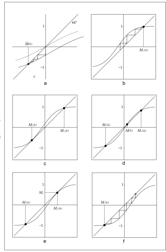
The next proposition, illustrated in Figures 1, 2 and 3, determines all possible globally stable, locally stable and unstable equilibria of difference of demand fractions of (24) depending on values assumed by Φ′(0)−1, J and h.
Note that, for a large class of parametric distribution functions, Φ′(0)−1 is an
increas-ing function of the standard deviation of the consumers’ intrinsic preferences, θ(i), i∈C,
whose distribution function is x7→Φ(x−θ). In particular, if Φ is the cumulative normal distribution with mean zero and varianceσ2, then Φ′(0)−1 is proportional to the standard
deviation σ of the consumers’ intrinsic preferences θ(i), i ∈ C, (Φ′(0)−1 = √2πσ).
Sup-posing such a suitable parametric form for Φ, we can interpret Φ′(0)−1 as a measure for
the heterogeneity in consumers’ intrinsic preferences for the establishments.
Our interpretation of (Φ′(0))−1 allows us to establish the relationships between the
consumer interactions (J), the heterogeneity of consumers’ intrinsic preferences (Φ′(0)−1)
and the resulting types of equilibria for the difference of demand fractions. In what follows, we will say, therefore, that
Proposition 2. Let Φbe a probability distribution function satisfying (7). Setg(m;h) := 2Φ Jm−h
−1 and denote by M := {m|m = g(m;h)} the set of equilibria of the dynamical system (24) (mt=g(mt−1;h), t ≥1). Denote by |M| the number of elements
of M. The following relationships hold for J ∈[0,∞) and h∈R:
1. If Φ′(0)−1 ≥2J
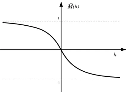
then |M| = 1 and the unique element of M, denoted by M¯(h), is a globally stable equilibrium of (24). Furthermore, the function h 7→ M¯(h) is decreasing, odd and continuous in h (with M¯(0) = 0). See Figure 1.a and 2 for this item.
2. If Φ′(0)−1 <2J
then there are critical thresholds h∗ >0 and M∗ >0 determined by
M∗ = 2Φ JM∗−h∗
−1
1 = 2Φ′ JM
∗−h∗
J
such that
(a) if −∞< h < −h∗
then |M| = 1, and the unique element of M, denoted by M+(h), is a globally
stable equilibrium of (24). See figure 1.b for this item; (b) if h=−h∗
then |M| = 2, and the elements of M, denoted by M−(−h) and M+(−h) are
such that: (i) M−(−h) = −M∗ <0 < M∗ < M+(−h); (ii) M−(−h) (=−M∗)
is an unstable equilibrium of (24) and its domain of attraction is [−1,−M∗];
(iii)M+(−h)is a locally stable equilibrium of (24) and its domain of attraction
is(−M∗,1]. See figure 1.c for this item;
(c) if −h∗ < h < h∗
then |M| = 3, and the elements of M, denoted by M−(h), M(h) and M+(h),
are such that: (i) M−(h) < −M∗ < M(h) < M∗ < M+(h), and (ii) M(h)
is unstable, while M−(h) and M+(h) are locally stable equilibria of (24); the
domains of attraction of M−(h), M(h) and M+(h) are [−1, M(h)), {M(h)}
and (M(h),1] respectively. See figure 1.d for this item; (d) if h=h∗
then |M| = 2, and the elements of M, denoted by M−(h) and M+(h) are
such that: (i) M−(h) < −M∗ < 0 < M∗ = M+(h); (ii) M−(h)is a locally
stable equilibrium of (24) and its domain of attraction is [−1, M∗]; (iii) M+(h)
(= M∗) is an unstable equilibrium of (24) and its domain of attraction is
(M∗,1]. See figure 1.e for this item;
(e) if h∗ < h <∞
then |M| = 1, and the unique element of M, denoted by M+(h), is a globally
(f ) M+(h) = −M−(−h) for all h ∈ (−∞, h∗], and M(h) = −M(−h) for all
h ∈ (−h∗,+h∗). Furthermore, the functions M+ : (−∞, h∗] → [−1,1] and
M : (−h∗,+h∗)→[−1,1] satisfy the following properties:
i. M+ : (−∞, h∗]→[−1,1] is decreasing and continuous,
ii. M : (−h∗,+h∗)→[−1,1] is increasing and continuous,
iii. limh→−∞M+(h) = 1 and M+(h∗) =M∗ = limh→h∗M(h)
See Figure 3 for this item.
Proof. The formal proof of Proposition 2 uses the the Implicit Function Theorem. What we present below is an informal but intuitive argument that support the assertion of the proposition.
The intuitive proof of Proposition 2 we are going to present uses the following three obvious facts. Firstly,mis an equilibrium of the dynamical systemmt = 2Φ(Jmt−1−h)−1
if and only if (m, m) is the interception point of the graph of the mappingm7→g(m;h) := 2Φ(Jm−h)−1 with the 45◦-line {(m, m) : m ∈ [−1,1]}. Secondly, the graph of m 7→
g(m;h) := 2Φ(Jm−h)−1 may be obtained from the graph ofm7→g(m; 0) := 2Φ(Jm)−1 by a horizontal shift by h/J. Thirdly, the graph of m 7→ g(m;h) has an ”S” shape, by which we mean the following three properties of the function m 7→ g(m;h): i) it is increasing and continuous; ii) it is bounded below by −1 and bounded above by +1; and iii) it is concave on (−∞, h/J] and it is convex on [h/J,∞).
We will divide the proof into the two cases:
1) Φ′(0)−1 ≥2J and 2) Φ′(0)−1 <2J.
Φ′(0)−1 ≥2J (Figures 1.a and 2 help to explain our arguments in this case):
When Φ′(0)−1 ≥ 2J, then the function m 7→ ∂g(m,0)/∂m attains its maximum at
m= 0, and∂g(m,0)/∂m|m=0 = 2JΦ′(0)≤1. Thus, (0,0) is the unique interception
point between the graph of m 7→ g(m; 0) (the dashed line in Figure 1.a) and the 45◦-line. Since the graph of m 7→ g(m;h), can be obtained by horizontal shifting
the graph of m 7→ g(m,0), it is easy to verify that for any h ∈ R, there is only
one interception between the graph ofm7→g(m;h) and the 45◦-line. Denoting this
interception by ( ¯M(h),M¯(h)) and shifting h from the left to the right, it is easy to observe graphically that h 7→ M¯(h) satisfies the properties stated in item (1) of Proposition 2. See the graph of h 7→ M¯(h) in Figure 2. That the domain of attraction of ¯M(h) is the whole intervale [−1,1] can be deduced from a graphical analysis as indicated with the zig-zag lines in Figure 1.a.
Φ′(0)−1 <2J (Figures 1.b-f and 3 help to explain our arguments in this case):
Contrary to the previous case, when Φ′(0)−1 <2J, we have here that∂g(m,0)/∂m|
m=0=
2JΦ′(0) > 1. From the ”S” shape of the graph of m 7→ g(m,0) it follows that
-are also three interceptions, (M−(h), M−(h)), (M(h), M(h)) and (M+(h), M+(h)),
with M−(h)< M(h)< M+(h), between the graph m7→ g(m, h) and the 45◦-line if
h does not lie far from zero, i.e., if|h|< h∗. If |h|=h∗ there are two interceptions,
(M−(h), M−(h)) and (M+(h), M+(h)), with M−(h) < M+(h). If |h| > h∗, there is
only one interception between the graphm 7→g(m, h) and the 45◦-line. Ifh <−h ∗,
we denote this interception by (M+(h), M+(h)); and, if h > h∗, we denote it by
(M+(h), M+(h)).
The assertions concerning the location of the equilibria M−(h), M(h) and M+(h)
can be deduced from the graphs of h 7→ M−(h), h 7→ M(h) and h 7→ M+(h)
illustrated in Figure 3. These graphs can be constructed by shifting the graph of m 7→ g(m, h) from the left to the right and observing the movement of the equilibrium in interest as illustrated in Figures 1.b-f. The domains of attraction of the equilibria ¯M(h), M−(h), M(h) and M+(h) are identified from the ”S” shape
of the graph of m 7→ g(m;h) applying a graphical analysis as indicated with the
zig-zag lines in Figures 1.b and 1.f.
6
Socioeconomic interpretation and applications
The contents of Proposition 1 and 2 allows us to viewmtas an approximation form( N,C)
t ,
when the population is large. Indeed, these propositions ensure that the distribution of the random variable m(tN,C) is concentrated around mt and that the probability of
the deviations of m(tN,C) from mt may be made as small as desired by the choice of an
appropriate number of consumers N. This implies that limt→∞mt may be viewed as
the time-stable difference of demand fractions of the establishments; to be precise: if the difference of demand fractions starts from some m(0N,C) =m0 and if we wait for a given
relaxation time until we see thatm(tN,C) is more or less constant in time, then the value of
m(tN,C)will be close to the limt→∞gt(m0;h). Since this limit is the subject of Proposition 2,
its results provide us with properties of the stable distribution of the consumers between the establishments and its dependence on the model parameters. These properties will be analyzed below from the socioeconomic point of view.
6.1
Interpretation of the model’s parameters
The results of Propositions 1 and 2 which we are going to interpret from the socioeconomic point of view involve the quantitiesJ, Φ′(0)−1 andh. The socioeconomic interpretations of
J and Φ′(0) have been already presented; recall thatJ gives the strength of social influence
among consumers, while Φ′(0)−1 expresses the heterogeneity of the consumer’s intrinsic preferences θ(i), i ∈ C. Here, we shall interpret the parameter h from a socioeconomic
point of view.
Recall we have defined θ :=p(+1)−p(−1), ¯θ :=E(θ(i)) andh:=θ−θ¯. Thus,
✁
✁
d
✂☎✄
✄
c
✁
✁
e
✂✆✄
✄
✂✆✄
✄
c
a
45 o
b
f ✂ ☎ ✄
✄
m
m
M
M
M M
M M M
M
M
M
M
In words, h is the expected value of the difference between the price difference θ =
p(+1)−p(−1) and the intrinsic preference θ(i) of a consumer i.
Recall, according to Remark 1 in Section 2, that the intrinsic preference θ(i) express
the preference of consumer i, when he/she is not affected by the social interaction; i.e., when both establishments are equally demanded, consumeri
1. prefers E(+) to E(−) if the price difference θ is below θ(i).
2. is indifferent between E(−) and E(+) if θ =θ(i).
3. prefers E(−) to E(+) if the price difference θ exceeds θ(i).
In the light of the three assertions above, we will call the quantityθ−θ(i)the consumer’s
i intrinsic excess price difference of the establishments E(+) and E(−). Accordingly, we
will call the expected value h=E(θ−θ(i))
the excess price difference of establishments (free from social influence)
Now, note that
P(θ−θ(i) >0) = P(θ−(θ+ξ(i))>0) =P(ξ(i) < θ−θ) = Φ(h) (25)
where, due to the symmetry of Φ′, we have: Φ(h) >1/2 (< 1/2) if h > 0 (h < 0). Note
also that, due to the continuity of Φ, we have: Φ(0) = 1/2.
Thus, the excess price difference h measures the advantage of one establishment over another. In fact, when the consumers suppose that both establishments are equally de-manded (equally attractive from social point of view), the following three relationships holds: i) ifh >0 then the majority of consumers will preferE(−) toE(+) (the exact
frac-tion of consumers that prefer E(−) to E(+) is Φ(h)>1/2); ii) if h < 0 then the majority
of consumers will prefer E(+) to E(−) (the exact fraction of consumers that prefer E(+)
to E(−) is 1−Φ(h) > 1/2); iii) if h = 0 then each establishment attracts 50% of the
consumers.
6.2
Two regimes of demand behavior
According to Proposition 2, the system (24) (mt = 2Φ(Jmt−1 −h)−1, t ≥ 1) has two
regimes:
Φ′(0)−1 ≥2J.
This is the regime where the heterogeneity of the consumers’ intrinsic preferences Φ′(0)−1 is relatively high compared with social influence on decisions J. We shall
call this regime
In this regime, there is only one stable difference of demand fractions ¯M(h)∈[−1,1] which is odd, decreasing and continuous in the excess price difference h ∈R. The
generic shape of the function h7→M¯(h) is given in Figure 2.
Φ′(0)−1 <2J.
This is the regime, where the heterogeneity of the consumers’ intrinsic preferences Φ′(0)−1 is relatively low compared with social influence on decisions J. We shall
call this regime
the low heterogeneity regime (Φ′(0)−1 <2J)
In this regime, the stable difference of demand fractions can acquire either one or two values,3 depending on the value of h. Figure 3 shows schematically this
dependence. M+(h) and M−(h) show the possible values of the stable difference of
demand fractions as functions of the parameterh, In particular, Figure 3 makes clear the following properties that will be important for our socioeconomic interpretation: the functions M+(h) andM−(h) are not defined for every h, and they co-exist for
h∈[−h∗, h∗]; moreover, M+ is always positive, while M− is always negative.
The different behaviors of the stable difference of demand fractions in our model and their dependence on the parameters Φ′(0)−1, J and h allow us to link the occurrence
of certain market phenomena with the degree of heterogeneity of consumer’s intrinsic preferences (Φ′(0)−1), the social influence on consumers’decision (J) and the excess price
difference of establishments (h). We shall do this in the following subsections.
6.3
Demand bubble
We stress that in the low heterogeneity regime (Φ′(0)−1 < 2J), the stable demand may
behave like a stable excess demand of an over-valued asset in a stock market.
Look at the branch of the graph of M+(h) that lies to the right of the vertical axis in
Figure 3. This branch shows that it is possible that the inequalitiesM+(h)>0 andh >0
occur simultaneously. Note that the inequality h > 0 means that if the consumers were not affected by social interactions, i.e., when they suppose that both establishments are equally demanded, then the majority of them would choose the establishment E(−). On
the other hand, the inequality M+(h)>0 means that the market is in the stable state in
which the establishment E(+) is more demanded than E(−).
We note that the demand bubble is impossible in the high heterogeneity regime (Φ′(0)−1 ≥2J). Figure 2 shows this fact clearly: the stable difference of demand fractions
¯
M(h) is negative when h > 0, and ¯M(h) is positive when h < 0. This means that E(−)
3Recall that Proposition 2 identifies stable and unstable equilibria of the dynamical systemm t+1 =
2Φ(J mt−1−h)−1. However, only stable equilibria will be viewed as possible values for the stable
M
Figure 2: Generic shape of the function ¯M(h) that represents the dependence of the globally stable equilibrium of the dynamical system mt+1 = 2Φ(Jmt−h)−1 on h in the
case Φ′(0)−1 ≥2J.
+✝
- ✞
M
M M
M
M
Figure 3: Generic shapes of the function M+(h), M(h) and M−(h) that represent the
dependence onhof the values of the equilibria of the dynamical systemmt+1 = 2Φ(Jmt−
is more demanded than E(+) whenever the excess price difference h is positive, and vice
versa.
6.4
Working either over or under capacity
When two similar establishments dominate a market, usually each is ready to absorb approximately 50% of the total amount of all virtual consumers of this market (effective consumers of both establishments + queue at the entrance of one of them). This is natural: each manager expects that approximately 50% of the virtual consumers will visit his establishment and the rest will visit the other one. Nevertheless, in real life, it may happen that one of the similar, competing establishments is almost empty, while the other one is full and there is always a queue at its door, even when both charge similar prices. We shall use our model to explain this apparent contradiction.
When both establishments are similar (in an extreme case, identical), it is natural to suppose that all consumers are intrinsically indifferent to both and thus θ(i) ≃ 0, i ∈ C,
implying that Φ′(0)−1 <2J. In what follows, we shall show that in the low heterogeneity
regime (Φ′(0)−1 < 2J), one of the establishments will always work under capacity and
the other one over capacity, whenever the capacity of each establishment corresponds to 50% of the total amount of all virtual consumers.
Let us define
N(+)(h) := (1 +M+(h))/2, and N(−)(h) := 1−N(+)(h) (26)
where h → N(+)(h) andh →N(−)(h) are defined in the domain of the stable difference
of demand fractions h→M+(h).
Note that N(+)(h) (resp.,N(−)(h)) is the fraction of the consumers that visit E(+)
(resp.,E(−)), when the difference of demand fractions has stabilized atM
+(h). The shapes
of the functions h → N(+)(h) and h → N(−)(h) are illustrated in Figure 4 and are
determined by the shape of function h→M+(h), illustrated in Figure 3.
Figure 4 illustrates clearly the fact that there is no excess price difference h for which the stable demand fractions of both establishments would be close to 50% of all virtual consumers (the total amount of N consumers). If both establishments have capacities close to 50% of all virtual consumers, i.e., if the relative capacities K(+) and K(−) of the
establishments E(+) and E(−) (absolute capacities divided by the total demand of both)
lie between 1/2−M∗/2 and 1/2 +M∗/2 as illustrated in Figure 4, then eitherE(+) works
over capacity and E(−) works under capacity, or vice versa.
We stress that the phenomenon just described does not occur in the high heterogeneity regime (Φ′(0)−1 ≥2J). In the high heterogeneity regime there is a unique globally stable
+✟
N N
K K
M
1 2
M
1 2
0
1 2
Figure 4: Graphs of h7→N+(+)(h) and h7→N (−) + (h).
6.5
Discontinuity of the stable demands and phase change
In this section we shall show that the stable difference of demand fractions is discontinuous in the excess price difference (h=θ−θ¯=p(+1)−p(−1)−θ¯) and consequently, that the stable demand fraction of each establishment is a discontinuous function of its price when the low heterogeneity regime prevails (Φ(0)−1 <2J).
We shall also show that the location of the discontinuity point of the stable difference of demand fractions depends on the initial difference of demand fractions at which the system mt+1 = 2Φ(Jmt −h)− 1 is at the initial time t = 0. We shall also use this
discontinuity to explain why some establishments do not raises their prices even when excess demand persists.
Let us introduce:
G(m0, h) := limt→∞gt(m0, h)
where gt(m0, h) is thet-th iteration ofm7→2Φ(Jm−h)−1 starting fromm0.
When Φ′(0)−1 < 2J, then the implications (27), (28) and (29) follow from
Proposi-tion 2:
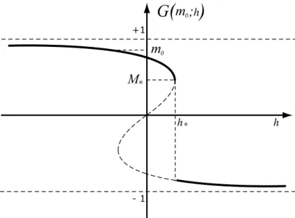
m0 > M∗ ⇒ G(m0;h) =
M+(h) if h≤h∗
M−(h) if h > h∗ (27)
(see Figure 5);
m0 <−M∗ ⇒ G(m0;h) =
M+(h) if h <−h∗
(see Figure 6);
−M∗ ≤m0 ≤M∗ ⇒ G(m0;h) =
M+(h) if h < M−1(m0)
m0 if h=M−1(m0)
M−(h) if h > M−1(m0)
(29)
(see Figure 7).
Discontinuity. Note that in all three cases m0 < −M∗, m0 > −M∗ and −M∗ ≤ m0 ≤
M∗, the function h 7→ G(m0;h) is discontinuous. In this sense, we say that the stable
difference of demand fractions is discontinuous in the excess price difference h. The consequence of the above discontinuity is given in the paragraph below.
Assume without loss of generality that the initial difference of demand fraction is at the stable equilibrium m0 = M+(h), with h < h∗. Note that (27) shows that a change
of the excess price difference from h to h+ ∆h, where h < h + ∆h < h∗, leads to a
new equilibrium atM+(h+ ∆h) after a certain relaxation time. When, however, the new
excess price differenceh+ ∆hexceeds the thresholdh∗, the difference of demand fractions
mt is attracted from M+(h) to the only remaining negative attractor M−(h+ ∆h), in
accordance with (27).
Phase change. Note that, in order to revert the equilibrium fromM−(h+∆h) toM+(h),
it is not sufficient to eliminate the increment ∆h. Due to the fact thatM−(h+ ∆)<−M∗
and the model symmetry, expressed in (28), a change of the excess price difference from
h+ ∆h to h, with −h∗ < h < h∗ < h+ ∆h, would lead to a new equilibrium at M−(h)
(and not at M+(h)). To drive the system to the equilibrium at M+(h) again, one needs
first to decrease the excess price difference from h+ ∆h to some h′ with h′ < −h ∗ and
then bring it back to h. That means that an uppercrossing of the discontinuity point h∗
causes not only a discontinuous jump in the current locally stable difference of demand fractions, but it causes also a phase change of the stable difference of demand fractions as a function of h.
Persistence of excess demand in real life. The discontinuity and the phase change mentioned above are consistent with Becker’s (1991) argument explaining why restaurants sometimes do not raise prices even when a certain excess demand persists.
+✠
- ✡
;
m
G
0m
0M
Figure 5: Graph of h7→G(m0;h) :=limt→∞gt(m0;h) form0 ∈(M∗,1).
of the mean intrinsic preference ¯θ) that could bring the excess price difference h below the new discontinuity point −h∗. To see this, consider (27) and (28) and recall that
M−(h)<−M∗, ∀h >−h∗ and M+(h)> M∗,∀h < h∗; and that h=p(+1)−p(−1)−θ¯.
7
Closing remarks
We end our discussion extending the explanation proposed by Gary S. Becker for the orig-inal problem that motivated the construction of our model. This problem was proposed by Gary S. Becker (1991) in the following way:
”A popular seafood restaurant in Palo Alto, California, does not take reservations, and every day it has long queues for tables during prime hours. Almost directly across the street is another seafood restaurant with comparable food, slightly higher prices, and similar service and other amenities. Yet this restaurant has many empty seats most of the time.
Why doesn’t the popular restaurant raise prices, which would reduce the queue for seats but expand profits ?”
In Section 6.5 we gave our explanation to this question. Here we would like to stress the fact that our explanation to this specific question uses the fact thetwo restaurant are similar in their service and amenities, and that they are placed close to one another.
+☛
- ☞
;
m
G
0m
0M
Figure 6: Graph of h7→G(m0;h) :=limt→∞gt(m0;h) form0 ∈(−1,−M∗).
+✌
- ✍
;
m
G
0m
0m
M 0 -1
intrinsic preferences, θ(i), i ∈ C, is relatively low. Hence, in the case of similar (in an
extreme, case identical) restaurants, it is natural to assume that the low heterogeneity regime (Φ′(0)−1 <2J) prevails.
Now, as explained in Section 6.4, under low heterogeneity of consumers’ intrinsic preferences, i.e, Φ′(0)−1 < 2J, one establishment may work under capacity, while the
other works over its capacity; even when both establishments charge the same prices. That the over demanded restaurant does not raise price is due to the profit maximization behavior in the presence of the discontinuity of demand, as explained in Section 6.5. This explanation is consistent with Gary S. Becker’s analyzes of demand behavior of two similar restaurants placed close to one an other.
In essence, the novelty of our explanation is that the similarity of the restaurants, i.e., the homogeneity of the consumers’s intrinsic preference for the restaurants, plays a key role in guaranteeing the phenomena just described.
Note that we also extend the analysis and results of the demand behavior of two establishments to the case when the establishments (or consumer choices) are dissimilar, i.e., when they represent two distinct consumption options for the population of consumers population. When the consumers are relatively heterogeneous in their intrinsic preferences for establishments (Φ′(0)−1 ≥2J), the two establishments will acquire the same level of
demand (N/2), whenever there is no excess price difference, i.e, whenever h= 0.
It seems, therefore, that the degree of heterogeneity in consumers’ intrinsic preferences plays a crucial role in determining the emergence of one or two phases of the demand fractions of the two establishments.
References
Becker, Gary S., 1991. A Note on Restaurant Pricing and Other Examples of Social Influences on Price. Journal of Political Economy 99/5, 1109-1116.
Brock, W. and Durlauf, S., 2000. Discrete Choice with Social Interactions. CSED Working Paper No. 18, University of Wisconsin at Madison.
Durret, R., 1995. Probability: Theory and Examples. 2nd ed. (Duxbury Press).