Working Paper
# 578
2013
Referenda
outcomes and the
influence of polls:
a social network
feedback process
Referenda outcomes and the influence of polls: a social
network feedback process
Ariel Guerreiro
a,band Jo˜ao Amaro de Matos
c15th November 2013
aDepartamento de F´ısica e Astronomia, Faculdade Ciˆencias Universidade do Porto, Rua do
Campo Alegre, 687 4169-007, Porto, Portugal
bINESC TEC - INESC Technology and Science (formerly INESC Porto)
c Nova School of Business and Economics, INOVA, Campus de Campolide, 1099-032, Lisboa,
Portugal
15th November 2013
1
Introduction
Voting is an intrinsic part of the modern concept of democracy and the desire to antecipate the polling results is every bit as ancient as the very notion of ballot casting. Polls sample information from the voting population to infer the dynamic evolution of the voters’ intention until the date of the elections. On the one hand polls are important ingredients for political strategists to center their efforts and resources in order to increase their share of votes. On the other hand some political analysts fear that polls may influence the outcome of the process. In many countries there are laws in place to prevent polling results from becoming publically available close to the election days, reflecting this concern. Also, several analysts claim that unexpected abstention may result from the perception of a clear winner based on polls, relaxing the motivation of individuals to vote. The level of abstention may clearly impact polls’ ability to predict the results of an election accurately.
We argue that although polls may accurately unveil the political preferences of the voters, sometimess they do a poor job of predicting the voters’ willingness to vote on election day. And yet, most of the time accuracy seems to be the dominant view; the Gallup polling organization, for example, has often been accurate in predicting the outcome of U.S. Presidential elections and the margin of victory for the election winner. However, it was off the mark in some close elections, such as in 1948 (predicting the victory of Republican Dewey over Democrat Truman), 1976 (a victory for Republican Gerald Ford over Democrat Jimmy Carter), and 2000 (Democrat Al Gore over Republican George W. Bush). In 1982 Los Angeles Mayor Tom Bradley lost the California gubernatorial race despite being ahead in voter polls going into the elections.
pre-election accuracy of polls (see Magalhaes, 2005) finds it comparable to that in other developed countries, suggesting that errors are caused by either the closeness of elections or a shared inability of pollsters to deal appropriately with the problems caused by low turnout (turnout in national elections has fallen from 98% in 1975 to less than 50% in recent years).
This phenomenon applies not only to general elections but also to other voting processes, such as referenda. In the recent past there have been a number of referenda in Portugal about several different political and social issues. The first referendum about the legalization of abortion was held in 1998 and a sequence of polls pointed out that the position in favor of legalization would win (see Fig. 1). Among 11 different polls (including some associated with the Catholic Church) during a period of two months, values ranged from 52% to 86% in favor of legalization.
[Insert Figure 1 here]
The surprising outcome of the referendum was a majority of valid votes (50.9%) against the legalization. However, far less than 50% of the population voted - only 31.9% - making the result legally non-binding. The experts argued that the repeated announcements of victory from “yes camp” reinforced the abstention clustering among the part of the population in favor of the legalization. On the contrary, people against legalization of abortion mobilized to vote.
Since the result was non-binding, a new referendum was called in 2007 (see Fig. 2). Although in the first referendum the opinion makers for legalization had focused their efforts on the discussion of the issue per se, in the second referendum their effort was complemented with a strong appeal to participation in the voting process. In the second referendum 59.25% of the valid votes were in favor and 40.75% were against, with a participation of 44% of voters, this time confirming the polls.
[Insert Figure 2 here]
at-tain the optimal individual decision. By public information we understand both the perception about the intentions of other voters, and also the information resulting from the public debate about the different issues at stake in the voting process. In a general election, noise is clearly generated by both, since public debate is spread across different topics. In the case of referenda, however, there is only one issue at stake and noise affecting the individual decisions can onlya-rise from the perception of voting intentions. In that sense, by applying our model to the case of referenda, we assume that incomplete information prevents voters from incorporating the expected abstention level in the update of their optimal voting decision, possibly preferring to abstain when they should ideally vote, or preferring to vote when they should ideally abstain. Second, there may be an asymmetric predisposition toward abstention among the individuals willing to vote for each of the different possible outcomes. Given that such a predisposition may be amplified by social interactions and the fact that the publicly available information of polls is incomplete, there is an interaction of these two features of decision making, possibly leading to stronger deviations from the forecast. This may lead not only to significant errors in the winning margin forecast but also to a reversed result, as in the Portuguese referenda example discussed above.
Our main research question is thus to understand how polls influence the final voting of individuals and may also ultimately affect the abstention level and their own forecast ability. The model answers to a non-trivial tradeoff faced by voters, namely how to take into account this feedback effect stemming from incomplete information while reducing the risk of having their stand misrepresented in the final voting result. Such strategic behavior leads some voters to incur the cost of voting with an eye to the benefits of the final result. This model has an additional appealing feature, namely the fact that it can be easily calibrated. Thus, it can be used to forecast results and be appropriately tested in a comprehensive way, allowing analysts to check their interpretation of surprising results.
compulsory, and information about the voting topic is widespread as a result of public debates and the agency of news media. Additionally, a sequence of public polls shows how the opinion of the electorate regarding the issue at stake trends over time. The choice of this referendum for our analysis is based on two reasons: first, the data were easily accessible, and second, and more importantly, there have been two referenda on the same topic - which is a rare occurence. This allowed for two different calibrations of the model, in the first referendum and the second a few years later. By comparing the different parameters obtained from the two calibrations, we may infer how the results affected the predisposition of voters to vote and abstain in the second referendum. We are thus able to explain why the results of the first referendum were so distant from forecasts and why the results of the second referendum confirmed all the forecasts, corroborating much of the political analysts’ belief. As stressed above, our model builds on two points: the incomplete flow of information provided by the sequence of polls and the social interactions that may amplify the misreading of these polls, leading to erroneous forecasts. The argument to build such a model must come from the understanding of how individuals, on the basis of polls, update their decision on why and how to vote at all.
The remainder of the paper is organized as follows. We first finish this section with a brief review of the literature. In the next section we lay out the model, followed by a section in which the results are presented and their implications analyzed. We then calibrate a linearized version of the model for the case of both abortion referenda in Portugal. The outcome of the calibration is analyzed in light of the arguments raised by the political analysts, strongly validating them. The last section presents our conclusions.
1.1
Literature review
recent reviews such as Dhillon and Peralta (2002), Feddersen (2004), and Gheys (2006). This is supported by empirical evidence reported in Cox (1997), Aldrich (1993), and Blais (2000, 2003), among others. Also a relatively recent literature (e.g. Klor and Winter, 2008, Grosser and Schram, 2010, Knight and Schiff, 2010) provides empirical and experimental evidence of the impact of polls in turnout and results of elections. By revealing updated information about the winning likelihood of the different platforms, some candidates gain momentum and others lose it, a mechanism that ends up giving much more comparative weight to the earliest polls than to the last ones.
In order to solve the original voting issue, Riker and Ordeshook (1968) evolved from Downs’ (1957) and Tullock’s (1967) subsequent work to suggest a consumption benefit from voting that, as pointed by Ferejohn and Fiorina (1975), would assume away the voting paradox. In this context, the decision to vote compares benefits and costs, taking into account the probability of being pivotal. Ledyard (1981, 1984) introduced a game-theoretical approach, making this probability endogenous, although ignoring voting costs. Palfrey and Rosenthal (1983, 1985) introduced costs in that game and concluded that when there is uncertainty about the actual number of voters, high turnout equilibria would not exist, since the probability that a vote is pivotal could be shown to be very small as the size of the voting population increases. Within the game-theoretical approach, Feddersen and Pesendorfer (1996, 1999) take an alternative route trying to understand why voters could possibly abstain under costless voting, and find that voters with strict preferences might abstain due to asymmetric information. This result does not explain the non-voting paradox, but brings the critical role of information to the decision-making process.
Harsanyi, 1977 and 1992; Kinder and Kiewiet, 1979; Markus, 1988; Coate and Conlin 2004; Feddersen and Sandroni 2006). Such group-based models have found empirical support (e.g. Schram, 1991 and 1992; Schram and Sonnenmans, 1996a,b; Hill and Leighley, 1996; Coate and Conlin, 2004), but cannot ensure (except for some very particular examples) the existence of equilibria or provide an endogenous mechanism that explains why an individual would join or be identified with any specific group, as pointed out by Feddersen (2004).
2
Model
Our model combines the strategic view of voting behavior with the feedback impact and is also based on a group-based reward, in the sense that we analyze aggregate behavioral outcomes (election turnouts together with the choice of the winner) when the behavior of voters exhibits social interaction effects. We follow the approach proposed by Brock and Durlauf (2001a, b) for the case of large elections. Individuals’ utilities are composed of a private utility associated with a choice and a social utility that reflects the desire to conform to others’ behavior in a non-cooperative decision-making setting. What is distinctive in this approach is that an individual’s choice is affected by the beliefs that the voter has about others’ intentions, as inferred from the polls’ results. The social interaction component of this model is thus reflected in the influence of the average of all the other voters’ attitudes, as expressed by the polls, on one’s own voting attitude. The choice model is closed by imposing self-consistency between the subjective beliefs and the objective probabilities conditional on the information made available by the polls, implying rational expectations. Brock and Durlauf (2001a,b) not only discuss the existence and stability of multiple equilibria in this model, but also show that in the presence of these conformity effects, the decentralized individual decision-making maximizes the aggregate social welfare. All such results are extended to a multinomial setting in Brock and Durlauf (2002, 2006), which is here suitably adapted and extended for the election model.
updated and the voting attitude of each individual is revised taking into account not only his or her private values, but also his or her desire to conform to others’ aggregate intended behavior. The voting decision in our model is taken as a result of the tradeoff of these effects. We assume that all voters’ attitudes are revised under the same updated information set and can prove that the final result of the process will converge to one of several possible multiple equilibria.
The comparative statics of our model are consistent with well-known empirical facts. Under complete information, the larger the lag between the proportion of favorable and unfavorable voters, the more comfortable the voters for the winning position will be, and the less important each of them will feel as a voter. The larger the announced gap, the less pivotal each voter feels, and the more willing he or she is to change his or her voting attitudes to abstention. On the contrary, the closer the gap in the polls, the less willing the voters are to abstain, since each voter becomes more pivotal. We show that under incomplete information this discrepancy between the forecast of the polls and the final results is aggravated, possibly inducing the type of reversed observed outcomes.
2.1
Modeling individual choice with private social utility
The electorate is modeled as a system with a large numberI of social agents, where each agent
i has to decide on a voting attitude to adopt ωi (e.g. ωi = 1 in favor, ωi = 2 to abstain, and
ωi = 3 against) by solving an individual utility maximization problem at some common time.
The space of all possible set of actions or decision outcomes taken by the population is the
N−tuple ω = (ω1, ...ωN). Also, ω−i = (ω1, ...ωi−1, ωi+1, ...ωN) denotes the set of the choices of all other agents except for the agentiitself. The individual utility, Vi(ωi), follows the structure
proposed by Brock and Durlauf (2001a) and is assumed to consist of three components
Vi(ωi;µei, ǫi) =U(ωi) +S(ωi, µei) +ǫi(ωi). (1)
The choice variable for agent i is the voting attitude ωi, which can take any value of the
under the conditional probability measure µe
i. The term µei ≡µei(ω−i) denotes the conditional probability measure that agent i places on the choices of the others at the time of making his or her decision. We shall denote by ω∗
i the actual outcome of the decision process of agent i,
ω∗
i =argmax Vi(ωi). The utility function of each agent takes into account not only individual
preferences expressed in the first term ui(ωi), but also information about the voting attitudes
of the other agents, expressed in the term Si(ωi, µei) and obtained from the publicly available
results of polls, which generate µe
i. The term ǫi ≡ ǫi(ωi) is a random contribution to the
utility that is observable to each agenti but unobservable to the modeler, and accounts for the heterogeneity of the different agents for each possible decision outcome ωi.
The voting attitudes are expressed as an overt behavior in two types of situations: when agents reply to poll queries and when they actually vote. It is assumed that polling takes place at an instant t prior to the decision process, which occurs at instantt+ 1, and that the public announcement of the results of the polls drives the agents to reevaluate their existing voting attitude. The outcome of the decision process is reflected only in later polls, say at instantt+2. A difference in poll outcomes at instants t and t+ 2 results from a reevaluation of individual voting attitudes at t+ 1, and so on. This describes a dynamic process in which the agents change their voting attitude until the referendum day, when their decision becomes definite.
From a collective point of view, the state of the system is described by the fraction of agents adopting the voting attitudes ωi = 1,2, and 3, respectively ∆1, ∆2, and ∆3 - or in a
compact vector form∆≡(∆1,∆2,∆3). By far most agents have no direct access to information
about the state of the system except through the results of the polls. These may introduce some distortion due not only to limitations in the sampling or polling methodologies, but also because the media that publicize the results may not provide a complete analysis of that information. For example, many media tend to focus on the relative percentage of agents in favor of or against, and neglect the level of abstention. The results of the polls are designated by m1, m2,
andm3- or in a compact vector formm≡(m1, m2, m3)-, corresponding to the frequencies of the
the fraction associated with abstention, the corresponding value of m2 is null, implying that
this information has no impact on the decision of the agent. Under these considerations, the dependence of the individual utility function Ui on µei is formally replaced by a dependency on
m, and it is thus possible to write
Vi(ωi) =U(ωi) +S(ωi,m) +ǫi(ωi). (2)
The first term denotes a deterministic private utility and is given by
U(ωi) =
3
X
α=1
uαδ(ωi, α) =
u1 if ωi = 1
u2 if ωi = 2
u3 if ωi = 3
,
thereby describing the individual preferences of each agent independently of the impact of the results of the polls. The constants uα, with α = 1,2 and 3, correspond to the expected
individual utility when the agent chooses the voting attitude α=ωi, ignoring the polls. Also,
the Kronecker delta is defined according to
δ(x, y) =
0 if x6=y
1 if x=y .
The second term of equation (2) denotes a deterministic social utility that models the stategic rationality of the agent when confronted with the results of the polls m. This term is given by
S(ωi,m) =
3
X
α=1
sα(m)δ(ωi, α) =
s1(m) if ωi = 1
s2(m) if ωi = 2
s3(m) if ωi = 3
,
polls. The functions sα(m) with α = 1,2,3 describes how the expected utility of an agent
depends on the results of the polls if the agent adopts the attitude α =ωi. The deterministic
part of the utility function is ¯
V(ωi,m) = U(ωi) +S(ωi,m) (3)
and can be written in a more compact and useful way as
¯
V(ωi,m) =
3
X
α=1
fα(m)δ(ωi, α) =
s1(m) +u1 if ωi = 1
s2(m) +u2 if ωi = 2
s3(m) +u3 if ωi = 3
(4)
where fα(m)≡sα(m) +uα is the utility specific for each potential voting decisionα.
The third term in equation (2) ǫi(ωi) denotes a random private utility, which is different for
each agent, thus modeling agent heterogeneity, and has the following structure
ǫi(ωi) =
3
X
α=1
ǫi,αδ[ωi, α] =
ǫi,1 if ωi = 1
ǫi,2 if ωi = 2
ǫi,3 if ωi = 3
,
where ǫi,α (with α = 1,2, and 3) are random independent variables, not necessarily equaly
distributed, the realizations of which may depend on the potential adopted attitudeωi.
Hence, the complete individual utility function becomes
Vt+1
i (ωi,mt) =
3
X
α=1
fα(mt) +ǫi,α
δ[ωi, α] =
f1(m) +ǫi,1 if ωi = 1
f2(m) +ǫi,2 if ωi = 2
f3(m) +ǫi,3 if ωi = 3
(5)
each quantity should be evaluated.
Each agent i chooses the alternativeω∗
i that provides his or her maximum utility, say
ω∗t+1
i =argmax ωi=1,2,3
Vt+1
i (ωi,mt).
Given that the individual utility function has a random component ǫi, one may only compute
the probability of each agent adopting an attitude ω∗
i =ωi, say
P(ω∗t+1
i =ωi) = P[Vit+1(ωi∗,m
t)≥Vt+1
i (ωi,mt),∀ωi = 1,2,3].
2.2
Pure herding effect
Consider the process of individual decision-making within a group, leading to a possibly different behavior for each member. We characterize a herd when the majority of the resulting behaviors are largely alligned, in spite of possible different personal preferences. In such a case individuals in the group act together without any planned direction, presenting a collective, relatively homogeneous, behavior. In the context of our decision-making model we would say that herd behavior occurs when the peer pressure described by the social utility part of equation (2) is greater than the private preferences as described by the first term. In this section we consider that the social utility component will reflect the gain of utility for an individual by agreeing with the choice of the other elements in the group.
In order to capture the herding effect, an increase of the utility of voting for a given alterna-tive α must follow as the polls reveal a larger fraction of voters in that same alternativeα. In other words, the function fα must be an increasing function of the fraction mα of agents
assu-med to adopt the positionα. For simplicity, the social interaction utility component describing the herding effect sh
α(mt) is assumed to be linear, say
shα(m) =aααmα, (6)
it follows that fh
α(m) = aααmα+uα and that
Vi(ωi,m) =
3
X
α=1
[aααmα+uα+ǫi,α]δ(ωi, α). (7)
2.3
Cross-herding effect
We now lead on to a more sophisticated version of the herding effect than the one considered above. Here we will consider that the decision of each agent is not only reinforced by the number of agents that agree with him or her, but also can be affected by the foreseen level of abstention. For example, agents who might prefer to abstain in the absence of the polls can be driven to conform to the winning side once the polls are public, thus reinforcing that position. This can also be captured by adopting a linear social interaction utility component, but now with a more complex structure, say
shα(m) =
3
X
β=1
aαβmβ, (8)
where the diagonal terms aαα (i.e. withα=β) correspond to the pure herding effect described
in the previous section, and the off-diagonal termsaαβ (withα6=β) describe the social pressure
between different voting attitudes, denoted here as a cross-herding effect. In this case the value of aαβ can be interpreted as the marginal increase in utility for an agent willing to vote for
alternative α if he or she aligns with voting for alternative β, reflecting a strategic voting behavior. The matrix a can thus be seen as a payoff matrix, leading each player to adopt a voting strategy that considers the aggregate decision of all other players. In this sense the herding effect with aαα > aαβ for α6=β can be understood as a coordination game.
It now follows that fh α(m) =
P3
β=1aαβmβ +uα and
Vi(ωi,m) =
3
X
α=1
" 3 X
β=1
aαβmβ+uα+ǫi,α
#
δ(ωi, α). (9)
differently on the sides of the “yes” and of the “no”, caused by an asymmetry in the parameters
a12 and a23 (or a21 anda32). As a consequence, one of the voting sides (“yes” or “no”) can drag
more undecided voters to their stand than the other, thus affecting the outcome of the polls and of the voting process.
2.4
From individual decisions to polls
The public information resulting from the polls at time t is described by the vector mt =
(mt
1, mt2, mt3) and is obtained by sampling the voting attitudes ∆t−1 = (∆1t−1,∆t2−1,∆t3−1) from
the population at time t−1. In a formal way, this is sumarized by
mt=R ∆t−1, (10)
where R is a function that describes how the information about the populations is sampled and converted into the public information made available to the voters, assumed to be a good estimator of µe(ω
−i). If this information is fully detailed about the state of the system, then it is possible to estimate the vector ∆≡∆t−1
1 ,∆t2−1,∆t3−1
bymt, say
mt=Rc ∆t−1≈∆t−1
1 ,∆t2−1,∆t3−1
, (11)
except for an estimation error.
However, if the public ignores the abstention level in their decision process because, for example, the media only publicize the percentage of voters in favor and against, then
mt =Ri ∆t−1 ≈∆t−1
1 ,0,∆t3−1
. (12)
This would make the contribution of the abstention level to the individual utility equal to zero. Another possible scenario occurs when the public is informed of the percentage of votes in favor and against corrected to the participation level of voters ∆1+ ∆2. The function R would
Ri∗ ∆t−1 =
∆t−1
1
∆t−1
1 + ∆t3−1
,0, ∆
t−1
3
∆t−1
1 + ∆t3−1
. (13)
Introducing equation (10) into the definition of the deterministic component ¯V of the indi-vidual utility function yields that
¯
V(ωi,mt) =
3
X
α=1
gα ∆t−1
δ[ωi, α] (14)
where gα ≡fα◦R1.
2.5
Formal solution of the utility maximization problem
Combining equations (10) and (9), and using the solution method described in appendix A, produces a relationship between the consecutive fractions of agents at instants t−1 and t+ 1
∆t+1
1 =
eβg1(∆t−1 )
eβg1(∆t−1)
+eβg2(∆t−1)
+eβg3(∆t−1) (15)
∆t2+1 = e
βg2(∆t−1)
eβg1(∆t−1)+eβg2(∆t−1)+eβg3(∆t−1) (16)
∆t+1
3 =
eβg3(∆t−1 )
eβg1(∆t−1)+eβg2(∆t−1)+eβg3(∆t−1) (17)
which can be written in a formal and compact way as
∆t+1
α =Fα ∆t−1
, with α= 1,2 and 3,
where Fα is defined by the right side of equations (15) to (17).
The Brouwer fixed point theorem (Brouwer, 1911) guarantees that this iteration process, in which the results of newer polls drive voters, converges to a fixed configuration of the system. This final configuration is an atractive fixed point of the discrete map transformation Fα,
1The symbol◦represents the function composition which is the application of one function (in this casef
α)
defined as
∆∗
α =Fα(∆∗). (18)
The Brouwer theorem also guarantees the existence of at least one fixed point but allows for more than one.
The populations for each voting attitude α satisfy the condition ∆1+ ∆2+ ∆3 = 1, which
allows writing the aggregate state of the system in terms of the participation level p= 1−∆2
and the polarization of opinions = ∆1−∆3. Equation (18) can be rewritten in terms ofp and
s as
st+1 = F1(∆t−1)− F3(∆t−1) (19)
pt+1 = 1− F
2(∆t−1). (20)
Equations (19) and (20) can be transformed into
st+2 = pt+2tanh[χ(st, pt)] (21)
pt+2 = cosh[χ(st, pt)]
cosh[χ(st, pt)] +1/2exp[ν(st, pt)] (22)
with χ(s, p) ≡ 1/2[g
1−g3], ν(s, p) ≡ g2 −1/2[g1 +g3] and gα ≡ gα(mt+1). It is convenient to
define the polarization of opinion adjusted to the level of participation as σt+2 ≡ st+2/pt+2.
Then, equations (21) and (22) can be written as
σt+2 = tanh[
e
χ(σt, pt)] (23)
pt+2 = cosh[χe(σt, pt)]
cosh[χe(σt, pt)] +1/2exp[χe(σt, pt)] (24)
against, the level of participation is fixed to 1 (i.e. pt+2 =pt= 1) and equation (21) reduces to
st+2 =tanh[χ(st,1)], (25)
which coincides with the expression obtained by Brock and Durlauf (2001a, 2001b) for a model with binary choice.
3
Results
In this section we characterize the types of fixed points of the system, as expressed in equation (18). This will characterize the outcome of the referendum according to our model. In a first step we consider only the case of herding effect in which information is complete and agents have access to the full results of the polls. In this case, R is given by the identity matrix as in equation (11). We next consider the case in which information is incomplete and agents ignore the abstention level. In this case R is given by equation (12). Finally, we address the case in which multiple outcomes are possible in each of the of the information settings described. In this case the usefulness of polls to forescast the referendum outcome is unclear.
3.1
Complete information
We consider the following model for the matrix aαβ in equation (8), reflecting the utilities for
the different voting attitudes in the case of complete information:
aαβ =
j q 0
q k r
0 r j
, (26)
where j is the utility if voters agree to vote in favor or against (since the herding effect should be equally strong in both directions), and k is the utility if voters agree to abstain. Parameters
The public information resulting from the polls is given by mt
β as in equation (10), which
can be obtained from the actual populations of agents according to mt β =
P
γRβγ∆tγ−1, where
R is the identity matrix. As a result, for complete information the utility function is simply ¯
V(ωi) =
3
X
α=1
" 3 X
β=1
aαβ∆tβ−1+uα
#
δ(ωi, α).
The outcome of the referendum, expressed as the percentage of the total number of valid votes that were in favor and against, is
%f avor = p+s 2p =
1
2(1 +σ) %against = p−s
2p =
1
2(1−σ).
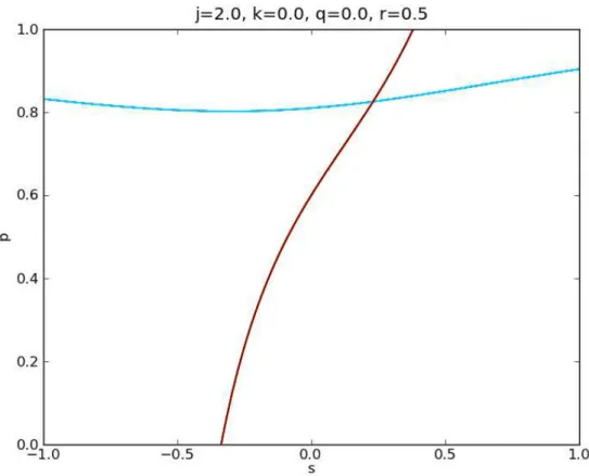
In Figure 3 we present an illustration of the stationary configurations of the system obtained as the overlap of the solution of equation (19) (drawn in red) and equation (20) (drawn in blue) for j = 2.0, k= 3.0,q = 0.0, andr = 1.0. In this situation there are different attitudes toward abstention. Voters in favor are indifferent to abstention (q = 0.0), whereas voters against are sensitive to the level of abstention (r= 1.0).
[Insert Figure 3 here]
From this figure, the fixed points resulting from this dynamic process are s = −0.10 and
p= 0.32, corresponding to 11% of votes in favor versus 21% against and an abstention level of 68%. This outcome translates into 34% of valid votes in favor and 66% against.
3.2
Incomplete information
We now consider the same model for the case of incomplete information with the same matrix
R =
1 0 0 0 0 0 0 0 1
.
Following equation (14), this results in a matrix ˜aαβ
˜
aαβ =
j 0 0
q 0 r
0 0 j
, (27)
which produces the same utility function as a complete information model with an adjusted matrix aαβ given by
aαβ =
j q/2 0 q/2 0 r/2
0 r/2 j
. (28)
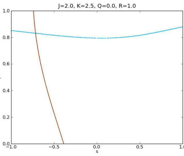
Using the participation levelp= 1−∆2and the polarization of opinions= ∆1−∆3, we present
an illustration of the stationary configurations of the system obtained for the same values of the parameters j = 2.0, k = 3.0, q = 0.0, and r = 1.0 as those used in the example above of complete information.
Under these conditions we have s= 0.23 and p= 0.82. As a result, the outcome translates into 64% in favor and 36% against, with a level of abstention of 18%. Comparing the results in Figures 3 and 4, we notice that under incomplete information there is a radical reduction of the abstention level (from 68% to 18%) as compared to the case of complete information, together with a change of the referendum result, from a rejection to an approval of the issue at stake.
[Insert Figure 4 here]
3.3
Multiple outcomes
satisfied. We now consider the case in which the parameters of the model are such that more of one pair can simultaneously satisfy both equations. This is illustrated in Figure 5, where on the left side we have cases of one single solution and on the right side the chosen parameters lead to three possible solutions.
[Insert Figure 5 here]
There are two features that we analyze in the Figure 5 graphs: i) the break of symmetry (visible in the change from the first to the second line); ii) the increase in the number of solutions (visible in the change from the left to the right side).
In the first feature, the two figures in the top line are perfectly symmetrical. The change to the bottom line breaks the symmetry of the solutions. From the point of view of the parameters,
q is different from r in the bottom line, reflecting different predispositions toward abstention between the two different groups. This means that one of the stands in the referendum provides a stronger motivation to vote - or to fight abstention - than the other stand. If we take the left column, we can see that this asymmetry favors one of the outcomes, namely the position of the group that is more mobilized to vote.
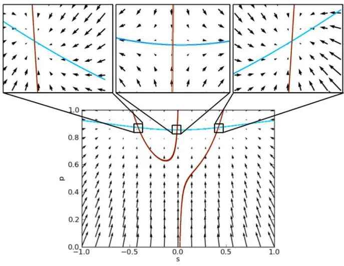
We also notice that in the cases corresponding to the right column of Figure 5 there is a third intermediate solution yielding a close match between the number of voters against and in favor. This basically corresponds to a tie or, more precisely, a state of indecision in which the system has not achieved a stable solution. In such a situation, a few people changing opinion may easily swing the solution to either one of the stable solutions. Even though this solution satisfies equations (19) and (20), and is a fixed point of the dynamics, it is unstable and very difficult to identify in real terms (see Figure 6).
[Insert Figure 6 here]
4
Calibration of the model
We now turn to an essential contribution of this approach. The issue we address here is to understand how the data gained from polls can be used to tell us something about the system that, in turn, will allow us to forecast the final result of the referendum with a satisfactory degree of accuracy. In other words, we would like to know the extent to which the sequence of poll data will allow us to correctly calibrate the model, determining the values of the parameters including the matrix a of interaction between voters and their individual preferences h.
Applying this procedure to the particular case of the abortion referendum in Portugal (1998), we will consider a matrix
aαβ =
j+ q 0
q k r
0 r j−
where we use two different parametersj: j+ for the social pressure among voters in favor, and
j− for the social pressure among voters against. For simplicity, we assume a generating function
G(y1, y2, ...) of the form
G(y1, y2, y3) = y1+y2+y3.
(1998), being careful not to include the results of the final referendum voting. We used non-linear minimum least square fitting to obtain
β×aαβ = 5.62×
8.28×10−2 2.34×10⁻¹ 0 2.34×10⁻¹ 4.58×10⁻⁷ −6.65×10⁻¹
0 −6.65×10⁻¹ 2.07×10⁻⁸
β×hα = 5.62×
8.81×10−3
−2.28×10⁻¹ 2.15×10⁻²
We notice several interesting things in this matrix.
First, the value of k is zero, meaning that the system behaves as if information were in-complete, in the sense that no emphasis was given in the media to the (declared) abstention level.
Second, the value of q is positive while the value of r is negative. This shows that voters against abortion were much more mobilized to vote than sympathizers of abortion legalization. This difference in mobilization actually could explain that most of the few final voters were against abortion, contradicting the polls. This is consistent with much of the subsequent ana-lysis in the press at that time, which sought to explain the surprising result of the referendum. We should also analyze the diagonal elements j+ and j−. Notice that the former is positive and the latter is zero for all practical purposes. Recalling that these numbers express the intra-group social pressure, we might expect that this simply reflects the fact that the arguments conditioning the attitudes of those in favor were strongly induced by social pressure. For those against, the arguments were clearly more of an idyosincratic nature, based on personal convictions that did not require reinforcement of social pressure.
β×aαβ = 1.58×
4.97×10−1 −3.56×10⁻¹ 0
−3.56×10⁻¹ 1.44×10⁻⁸ −5.00×10⁻¹ 0 −5.00×10⁻¹ 3.37×10⁻⁸
.
β×hα = 1.58×
3.08×10−2
−2.83×10⁻¹ 1.05×10⁻²
In light of the above analysis, it is clear what happened in this second referendum. In qualitative terms the only change in the matrix is that the value of q is now negative. This simply means that the group in favor changed their attitude toward abstention, becoming much more active in mobilizing people to vote. This is consistent with the explanation advanced by the analysts following the first referendum, that the outcome contradicting the polls resulted from a low mobilization of the majority of voters, namely those in favor.
5
Static and dynamic analysis
We now provide some comparative statics of the solution of the model matrix, say
β×aαβ =
j+ q 0
q 0 r
0 r 0
. (29)
Notice that in this matrix the values of k and j− have been set to zero in acordance with the results of the calibration described in the previous section. For this situation the functions in equations (23) and (24) become
e
χ(σ, p) = 1
4j+p(σ+ 1) + 1
2Γ(1−p) (30)
e
ν(σ, p) = 1
4j+p(σ+ 1) + 1
where Γ≡(q−r)/2 and Λ≡(q+r)/2 denote respectively the asymmetry and average in the cross-herding power toward abstention between voters against and in favor.
Consider first how small changes of the polarization of opinionδσtand of the voter
partici-pation δpt at instant t produce variation of the voters’ decision at instant t+ 2, namely δσt+2
and δpt+2:
δσt+2 = h1− σt+22i 1
4j+p
tδσt+h1− σt+22i 1
4j+(σ
t+ 1)−Γ
δpt (32)
δpt+2 = pt+21−pt+2
1 4j+(σ
t+2+ 1)−Γ
ptδσt+
+1 4p
t+21−pt+2 j
+(σt+2+ 1)(σt+ 1)−Γ(σt+2+σt)−2Λ
δpt (33)
In the neighborhood of each fixed point, the variation of the results of polls becomes small, and it then follows that δσt+2 ≈σt+2−σt,δpt+2 ≈pt+2−pt,σ ≈σt+2 ≈σt and p≈pt+2 ≈pt.
The feedback effect for σ between instantst and t+ 2 is given by
δσt+2 =1−σ21
4j+p δσ
t
(34)
and is always positive (δσt>0 implies thatδσt+2 >0), indicating a herding effect that reinforces
the results of the previous polls. On the other hand, the feedback effect for pbetween instants
t and t+ 2 is given by
δpt+2 = 1
4p[1−p]
j+(σ+ 1)2−2Γσ−2Λ
δpt. (35)
The analysis of this feedback does not have a well-defined signal, being positive forj+(σ+ 1)2−
2Γσ−2Λ > 0 and negative for j+(σ+ 1)2 −2Γσ−2Λ < 0 . To explain the meaning of the
change of sign ofδpt+2 assume for simplicity that Γ is positive and large (Γ/j
+ >2) and Λ = 0.
close to 1, and it is foreseen that the stand in favor is going to win with a large majority, some of these voters will tend to abstain, resulting in a negative feedback (δpt+2/δpt < 0). These
negative feedbacks are very interesting dynamically because they entail that the variations of participation will change sign in two consecutive polls, meaning that the participation level fluctuates (decreasing after increasing and vice-versa). This latter result can be interpreted as a reaction to a decrease in the perceived pivotal power of voters both in favor and against. For 0<Γ/j+ <2 the effect of cross-herding toward abstention of the voters in favor is not strong
enough to switch the sign of the feedback for largeσ but only a decrease amplitude ofδpt+2/δpt.
For negative Γ/j+ the cross-herding power is stronger for voters against and now occurs the
symmetrical case, where for large negative σ the participation fluctuates and for weakly and positive σ there is always a positive feedback.
The impact of the level of participation in the polarization or gapσbetween voting attitudes
w= 1 andw= 3 is obtained from
δσt+2 =1−σ2
1
4j+(σ+ 1)−Γ
δpt. (36)
In the absence of asymmetry toward abstention between voter in favor and against (Γ = 0), increases in participation level p tend to amplify the gap g and therefore the trend of the polls at t are reinforced at t+ 2. When an asymmetry is introduced (Γ6= 0) this amplification can be either increased (Γ<0) or decreased (Γ>0), and even inverted (Γ> 14j+(σ+ 1)).
The level of participation pis affected by the gap g according to
δpt+2 =p2(1−p)
1
4j+(σ+ 1)−Γ
p δσt. (37)
the participation level.
6
Conclusions
In this paper we propose an explanation for differences between the polls projections and the final outcome of referenda. Our model implies that there is a dynamic feedback between the results of polls and individual voting attitudes. This process can be affected by the way results of polls are presented to the public in the media and, ultimately, by the way they are perceived by voters. Dissonances between individual perception and aggregate voting trends can be amplified by the feedback process, resulting in a strong discrepancy between the results of polls and the actual voting outcome.
One such dissonance can occur when individuals within each of the voting groups have different predispositions toward abstention. This bias may not be explicit in the results of the polls as divulged by the media, which are more focused on the number of voting intentions in favor and against. Individuals are then not able to correctly anticipate the behavior of others in elections, and adjust their voting attitude accordingly. This can favor smaller voting groups with larger aversion toward abstention and eventually switch the outcome of the referendum from the polls’ predictions.
From the dynamic point of view, we have shown that this model always has at least one attractive fixed point at which the number of individuals adopting each voting attitude is stable. The results of successive polls drive the aggregate voting attitudes and asymptotically converge to the attractive fixed point.
Under certain conditions, the model can have more than one fixed point, and it is then impossible to determine ex-ante the fixed point towards which the aggregate voting attitudes will converge. This can further frustrate polls in forecasting the outcome of referenda.
had pointed strongly in the opposite direction. At the time, many political analysts justified this discrepancy with a stronger predisposition to vote among individuals against the issue. The debate following the results of this referendum increased the social pressure for voters in favor not to abstain in the second referendum. Also, there was a more intense discussion of the impact of level of abstention in the voting results. In the voting results of 2007 the stand in favor had the largest number of votes, thus confirming the original polls.
Using the results of the polls in the run-up to each referendum, it is possible to calibrate the model incorporating cross-herding effects. For the parameters characterizing such effects, it was found that their values were consistent with the above-mentioned interpretation of the results. In particular, the calibration of the model provides evidence that voters in favor reduced their predisposition toward abstention following the 1998 results, leading to greater participation in the 2007 referendum.
different from the poll forecast.
Figures
Figure 3: Graphic determination of the stationary configuration of a social system of voters as solutions of equations (19) (drawn in red) and (20) (drawn in blue), for parameters j = 2.0,
Figure 4: Graphical determination of the stationary configuration of a social system of voters as solutions of equations (19) (drawn in red) and (20) (drawn in blue), for parameters j = 2.0,
Figure 6: Graphic determination of the stationary configuration of a social syste of voters as solutions of equations (19) (drawn in red) and (20) (drawn in blue), in a case with multiple stationary points. The arrows connect two consecutive configurations according to the dynamics of the system. On top we present amplifications of the graph in the proximity of each of the stationary points. It is shown that the two outer stationary points are stable while the central one is unstable.
Appendix A
McFadden (1978, 1981) developed a method for solving the maximization problem
ω∗t+1
i =argmax ωi=1,2,3
Vt+1
in a wide class of situations. His approach begins by considering that the random term of the individual utility functionǫi,αfollows a frequency distribution obtained from generating function
G ≡ G(y1, y2, ...). The function G is assumed to be a non-negative homogenous function of
degree d > 0 defined on the orthant yα ≥ 0, which diverges without bound. The kth cross
partial derivatives of G are non-negative when k is odd and non-positive when k is even. The valid multivariate distribution function generated by G is
FG=exp[−G(y1, y2, ...)]. (39)
McFadden (1978, 1981) showed that ifǫi,αjointly follows this type of multivariate generalized
extreme value with generating functionG, the probabilityP(ω∗t+1
i =ωi) can be derived in closed
form as
P(ωi = 1) =
y1G1(y1, y2, ...)
G(y1, y2, ...)
,
P(ωi = 2) =
y2G2(y1, y2, ...)
G(y1, y2, ...)
,
P(ωi = 3) =
y3G3(y1, y2, ...)
G(y1, y2, ...)
,
with yα =exp[βfαt], Gα =∂G/∂yα, and β some scalar parameter. A more recent formulation
of these results can be found in Misra (2005).
It is convenient to distinguish between individual quantities refering to a particular agent
i, say Xi ≡ Xi(ωi), which depend on the state of the agent alone, and global quantities X ≡
PN
i=1piXi, which aggregate individual quantities of all the agents according to some weights
pi.
The average value ofXi over the probability distributionP(ωi) for an individualiis defined
as the quantity
hXii=
3
X
α=1
and can be calculated using an aternative expression obtained by construction as
hXii=
∂ln G ∂Y Y=0 = 3 X α=1
Xi(α)eXi(α)Y
yαGα
G Y=0 = 3 X α=1
Xi(α)
yαGα
G =
3
X
α=1
Xi(α)P(α)
Following the same approach, the variance of Xi is
var(Xi)≡
Xi2
− hXii2 =
∂2ln G
∂Y2 Y=0 .
Also, the mean value of global quantities X can be computed by
hXi= ∂ln G
∂Y Y=0 = N X i=1 pi " 3 X α=1
Xi(α)
yαGα
G
#
.
In particular, the value ofh∆ican be calculated using the fact that ∆t+1
α =N−1
PN
i=1δ(ωi, α)
(i.e. with pi = 1/N and Xi =δ(ωi, α) ). Then
∆t+1
α = N X i=1 pi " 3 X β=1
Xi(α)
yαGα
G # = N X i=1 " 3 X α=1
δ[α, ωi]
yαGα
G
#
= yωGω
G . (40)
In the right side of equation (40) there is an implicit functional dependence of h∆t+1
w i in the
results of polls obtained at t via yα =exp[βfα(mt)] = exp[βgα(∆t−1)].
This dependence can be expressed in a formal way as
∆t+1
α
=Fα(mt) (41)
with Fα(mt)≡yαGα/G. To simplify notation, the average brackets hiare omited elsewhere in
this article.
References
[2] Blais, Andre, 2000, “To Vote or Not to Vote: The Merits and Limits of Rational Choice Theory”, Pittsburgh: University of Pittsburgh Press.
[3] Brock, W. and S. Durlauf, 2001a, “Discrete Choice with Social Interactions”, Re-view of Economic Studies, 68(2), pp. 235-60.
[4] Brock, W. and S. Durlauf, 2001b, “Interactions-Based Models”, in J. Heckman and E. Leamer, eds., Handbook of econometrics, Vol. 5. Amsterdam: North- Holland, pp. 3297-3380.
[5] Brock, W. and S. Durlauf, 2002, “A Multinomial-Choice Model of Neighborhood Effects”, The American Economic Review, Vol. 92, No. 2, pp.298-303.
[6] Brock, W. and S. Durlauf, 2006, “Multinomial Choice with Social Interactions”, in Blume, L, Durlauf, S. (Eds.), The Economy as an Evolving Complex System. 3, Oxford University Press, Oxford.
[7] Brouwer, L. E. J., 1911, “ ¨Uber Abbildung von Mannigfaltigkeiten”, Mathematische Annalen, Volume 71, Issue 1, pp 97-115.
[8] Coate, Stephen, and Michael Conlin, 2004, “A Group Rule Utilitarian Approach to Voter Turnout: Theory and Evidence”, American Economic Review 94(5) 1476-1504.
[9] Cox, Gary W., 1997, Making Votes Count. Cambridge: Cambridge University Press.
[10] Dhillon, A. and S. Peralta, S. 2002, “Economic Theories of Voter Turnout”, Eco-nomic Journal, 112 (June), 332-52.
[11] Downs, Anthony. 1957, An Economic Theory of Democracy, New York: Harper and Row.
[13] Feddersen, Timothy J. and Wolfgang Pesendorfer, 1996, “The Swing Voter’s Curse”, American Economic Review. 86:3, pp. 408-24.
[14] Feddersen, Timothy J. and Wolfgang Pesendorfer, 1999, “Abstention in Elec-tions with Asymmetric Information and Diverse Preferences”, American Political Science Review. 93:2, pp. 381-98.
[15] Feddersen, Timothy J. and A. Sandroni, 2006, “A Theory of Participation in Elec-tions”, American Economic Review, 96 n.4, 1271-1282.
[16] Ferejohn, John A. and Morris P. Fiorina, 1975, “Closeness Counts Only in Horse-shoes and Dancing”, American Political Science Review. 69:3, pp. 920-25.
[17] Geys, B., 2006, “‘Rational’ theories of voter turnout: a review”, Political Studies Review 4(1), 16-35.
[18] Goodin, R.E. and K. Roberts, 1975, “The ethical vote”, American Political Science Review 69: 926-928.
[19] Grosser and Schram, 2010, “Public Opinion Polls, Voter Turnout, and Welfare: An Experimental Study”, American Journal of Political Science, Vol. 54, No. 3 (July 2010), pp. 700-71.
[20] Harsanyi, John, 1977, “Morality and the Theory of Rational Behavior”, Social Research. 44:4, pp. 623-56.
[21] Harsanyi, John, 1992, “Game and Decision Theoretic Models in Ethics,” in The Handbook of Game Theory, Volume 1, R. Aumann and S. Hart, eds. Amsterdam, The Netherlands: Elsevier, North-Holland.
[23] Hill, Kim Quaile and Jan E. Leighley. 1996, “Political Parties and Class Mobili-zation in Contemporary United States Elections”, American Journal of Political Science. 40:3, pp. 787-804.
[24] Kinder, Donald R. and D. Roderick Kiewiet. 1979, “Economic Discontent and Political Behavior: The Role of Personal Grievances and Collective Economic Judgments in Congressional Voting”, American Journal of Political Science. 23:3, pp. 495-527.
[25] Klor, Esteban F. and Eyal Winter, 2008, “On Public Opinion Polls and Voters’ Turnout”, Hebrew University of Jerusalem, working paper.
[26] Knight, B. and N. Schiff, 2010, “Momentum and Social Learning in Presidential Primaries”, Journal of Political Economy, 118(6), 1110-1150.
[27] Ledyard, John, 1981, “The Paradox of Voting and Candidate Competition: A General Equilibrium Analysis”, in Essays in Contemporary Fields of Economics. George Hoorwich and James P. Quick, eds. Lafayette: Purdue University Press, 54-80.
[28] Ledyard John, 1984, “The pure theory of large two candidate elections”, Public Choice 44, 7-41.
[29] Magalh˜aes, P. C., 2005, “Pre-Election Polls in Portugal: Accuracy, Bias, and Sources of Error, 1991–2004”, International Journal of Public Opinion Research, 17 (4), 399-421.
[31] McFadden, D., 1978, “Modelling the Choice of Residential Location”, in A. Karl-qvist, L. LundKarl-qvist, F. Snickars, and J. Weibull, eds. Spatial Interaction Theory and Planning Models, Amsterdam: North Holland.
[32] McFadden, D., 1981, “Econometric Models of Probabilistic Choice”, in C.F. Manski and D. McFadden, eds. Structural Analysis of Discrete Data with Econometric Applications, MIT Press: Cambridge, MA, 198-272.
[33] Misra, S., 2005, “Generalized Reverse Discrete Choice Models”, Quantitative Mar-keting and Economics, 3, 175-200.
[34] Morton, Rebecca, 1987, “A Group Majority Model of Voting”, Social Choice and Welfare. 4:2, pp. 117-31.
[35] Morton, Rebecca, 1991, “Groups in Rational Turnout Models”, American Journal of Political Science. August, 35, pp. 758-76.
[36] Mueller, Dennis C., 2003, Public Choice III. Cambridge: Cambridge University Press.
[37] Palfrey, Tom and Howard Rosenthal, 1983, “A Strategic Calculus of Voting”, Public Choice. 41:1, pp. 7-53.
[38] Palfrey, Tom and Howard Rosenthal, 1985, “Voter Participation and Strategic Uncertainty”, American Political Science Review. 79:1, pp. 62-78.
[39] Riker, William and Peter Ordeshook, 1968, “A Theory of the Calculus of Voting”, American Political Science Review. March, 62, pp. 25-42.
[40] Shachar, Ron and Barry Nalebuff, 1999, “Follow the Leader: Theory and Evidence on Political Participation”, American Economic Review. 89:3, pp. 525-47.
[42] Schram, A.J.H.C., 1992, “Testing Economic Theories of Voter Behavior Using Micro-Data”, Applied Economics. 24:4, pp. 419-28.
[43] Schram, A.J.H.C. and J. Sonnemans, 1996a, “Voter Turnout and the Role of Groups: Participation Game Experiments”, International Journal of Game Theory. 25:3, pp. 385-406.
[44] Schram, A.J.H.C. and J. Sonnemans, 1996b, “Why People Vote: Experimental Evidence”, Journal of Economic Psychology. 17:4, pp. 417-42.
[45] Tullock, Gordon, 1967, Towards a Mathematics of Politics, Ann Arbor: University of Michigan Press.
Nova School of Business and Economics


![Figure 3: Graphic determination of the stationary configuration of a social system of voters as solutions of equations (19) (drawn in red) and (20) (drawn in blue), for parameters j = 2.0, k = 3.0, q = 0.0, r = 1.0, and h ≡ [h 1 , h 2 , h 3 ] = [0.2, 0., 0](https://thumb-eu.123doks.com/thumbv2/123dok_br/15728801.633706/32.892.129.662.372.815/figure-graphic-determination-stationary-configuration-solutions-equations-parameters.webp)