Limited attention and investor disagreement: a nowcasting approach

LIMITED ATTENTION AND INVESTOR

DISAGREEMENT: A NOWCASTING APPROACH

Gustavo Antonio De Cicco Pereira

LIMITED ATTENTION AND INVESTOR

DISAGREEMENT: A NOWCASTING APPROACH

Gustavo Antonio De Cicco Pereira

Dissertação submetida como requisito parcial para conclusão do Mestrado em Economia

     Ficha catalográfica  elaborada pela Biblioteca Mario Henrique Simonsen/FGV 

       Pereira, Gustavo Antonio De Cicco 

       Limited attention and investor disagreement: a nowcasting approach / Gustavo          Antonio De Cicco Pereira. – 2015.  

      32 f.    

       Dissertação (mestrado) ­ Fundação Getulio Vargas, Escola de Pós­Graduação          em Economia.   

      Orientador: Caio Ibsen Rodrigues de Almeida.        Inclui bibliografia. 

      1. Teoria da informação em finanças. 2. Mercado financeiro. 3. Investimentos.         4. Modelos econômicos. I. Almeida, Caio Ibsen Rodrigues de. II. Fundação Getulio         Vargas. Escola de Pós­Graduação em Economia. III. Título. 

      CDD – 332   

Agradecimentos

Agradeço ao Professor Caio Almeida por toda orientação e apoio, neste e nou-tros projetos. Ao Professor Marco Bonomo, pelas discussões que ajudaram a dar um rumo a este trabalho. Ao Professor Felipe Iachan, pelas sugestões e comentários valiosos.

Resumo

Quando a discordância em modelos econômicas ocorre devido a interpreta-ções diferentes de sinais públicos, o nível de “discordância de mercado” não necessariamente diminui com a chegada de um sinal público. Nós propomos uma avaliação empírica desse fenômeno. Usando uma medidade de atenção baseada no Google Trends, mostramos que um aumento na atenção alocada pelo mercado a uma company está associada a um aumento significativo da discordância sobre ela.

Abstract

When disagreement in economic models occurs due to different interpreta-tions of public signals, the level of “marketwide disagreement” not necessar-ily decreases upon the arrival of a public signal. We propose an empirical assessment of this phenomenon. By using a measure of attention based on Google Trends, we show that an increase in the attention allocated by the market to a company is associated to a significant increase in disagreement about it.

List of Figures

1 Abnormal returns when disagreement is or is not resolved after earnings announcement . . . 13 2 Google Search Volume in time for randomly

se-lected companies . . . 14 3 Abnormal Search Volume in time for randomly

Contents

1 Introduction 10

2 Related literature 11

3 Methodology 13

3.1 Regression strategy . . . 18

4 Results 20

4.1 One-year forecast horizon . . . 20 4.2 Two-year forecast horizon . . . 21 4.3 Interpretation of results . . . 24

5 Conclusion 28

Limited attention and investor disagreement: a

nowcasting approach

Gustavo Pereira

1

Introduction

It is evident from simple introspection that people are exposed to much more informa-tion than they can handle, especially in modern times. This fact has been documented in the behavioral psychology literature1 _{, but until recently, there was no single,} ac-cepted way to frame this idea in economic and financial models. The pioneering works of Sims [2006, 1998], by using concepts in Information Theory such asentropyand Shan-non capacity, provided an elegant mathematical formulation of the situation where the learning process of agents is such that there is a limit to the amount of information they can process per time period. This feature – subsequently called “rational inattention”– was successfully incorporated in macroeconomic models, and important insights have been obtained.2

In finance, the Information Theory approach has been used to modellimited atten-tion, i.e., the idea that agents cannot pay attention to all available information about assets in a given period. Together with the assumption that agents overestimate the accuracy of their own information, this approach has yielded testable implications, many of which seem to conform to the data. However, one important aspect of the fi-nancial markets that has been heretofore unadressed by the limited attention literature3 is that ofdisagreement. It has been shown in the standard framework – that is, where learning is costless – that differences of opinion can help explain several features of the financial market.4 _{If one is to add disagreement to the limited attention framework,}

1_{We refer the interested reader to the discussion by Hong et al. [2007]. See section I.} 2_{See Woodford [2001], Reis [2006a], Reis [2006b], Ball et al. [2005].}

3_{To the best of our knowledge.}

4_{See the literature review for more details.}

one fundamental question that needs to be addressed is: what happens to the “level of disagreement” when many agents simultaneously look at public information about the same asset? In other words: is there a tendency for beliefs to “converge”? The empirical analysis done in this thesis suggests that disagreement about the short term performance of a company5 _{increases when agents are simultaneously “consuming”} public information about it. We find no effect of increased attention on the disagree-ment about medium term performance of companies.

To get to this result, we use the dispersion of analyst forecasts in the I/B/E/S database6_{as a proxy for marketwide disagreement, and the volume of Google searches} about a company as a proxy for the attention allocated to it. We then estimate a static panel regression of disagreement against attention, and conclude that an increased at-tention to a company is significantly associated to a higher level of disagreement about it, even when aggregate uncertainty is controlled for. As we do not control for firm-specific uncertainty, there is the possibility that some underlying uncertainty compo-nent driving the disagreement is also causing Google searches to increase, and that this component is not being captured by the firm fixed-effects.

This thesis is organized as follows. In the next section, we briefly review the part of the literature on disagreement and limited attention that is connected to our thesis, as well as similar empirical analyses previously carried out in the literature. Subse-quently, we present a detailed account of our empirical methodology, as well as the results obtained. We then conclude by linking our results to the disagreement and limited attention literatures.

2

Related literature

Models in which agents are allowed to “agree to disagree” about relevant parameters have been used to explain many empirical regularities in the financial markets. These include the trading frenzy set off when earnings announcement are released [Harris and Raviv, 1993, Kandel and Pearson, 1995], the overpricing of financial assets [Har-rison and Kreps, 1978, Miller, 1977], the dynamics of the trading volume of options [Buraschi and Jiltsov, 2006], the correlation risk premium [Buraschi et al., 2014], and many others.

The branch of the disagreement literature in which we are mainly interested is the one where the parameter about which agents disagree is the interpretation of public signals, a phenomenon we hereinafter call “differential interpretations”.7 _{The models}

5_{The “performance” measure here is earnings-per-share, or EPS hereinafter.} 6_{Institutional broker estimate system.}

7_{By “interpretation” we mean the following. Suppose that an agent is trying to learn the true value of}

proposed by Harris and Raviv [1993] and Kandel and Pearson [1995] are the most common examples of this mechanism.8 _{The appeal of these papers is that both of them} conform to a great deal of empirical evidence concerning the joint behavior of volume and prices (or returns) of stocks. Additionally, Kandel and Pearson [1995] also give compelling arguments as to why prior models that relied on common interpretations were not consistent with novel empirical evidence. Despite the substantially different modelling ingredients used in both papers,9_{since the “common denominator” of these} models is the differential interpretations assumption, it seems fair to conclude that this might be an important mechanism.

Along with the importance of this assumption, a fact that we want to stress for the rest of this thesis is that, when differential interpretations are present, the level of disagreement typically increases when agents simultaneously observe a public signal; or, at least, a bigger disagreement is not automatically ruled out by force of the as-sumptions. Since the mathematical details are not of central importance, we leave an example of how different interpretations lead to an increase in disagreement upon the observation of a public signal to Appendix A.

Now, as has been argued in the introduction, agents cannot possibly process all the available public information in a given period in order to learn about the rele-vant states. The question of how the heterogeneity of beliefs would behave in a con-text where learning is subject to attention constraints has not been, to the best of our knowledge, addressed by the literature. What we seek to better understand with our empirical analysis is whether the differential interpretations assumption makes sense in a limited attention environment.

The closest model we have found is that of Peng and Xiong [2006], in which the dividends of risky assets have three independent components: market, sector, and firm-specific. Every period, a representative agent chooses how much of a fixed “at-tention endowment” she is willing to allocate on each of the uncertainty sources. The fact that they use a representative agent rules out heterogeneous beliefs by hypothesis. Nevertheless, their framework allows us to formulate the empirical analysis carried out in this thesis in more rigorous terms. We are interested in the reaction in differ-ences of opinion about a firm’s fundamentals when many agents are simultaneously allocating attention to that company.

an unobservable stateθ∈Θ_{, e.g., the future payoff of a company’s stock. All she can observe, however,}

is a signalswhichshe thinksis correlated toθ. Herinterpretationis defined to be what she believes is the distribution ofsconditional onθ(which she subsequently uses to infer the posterior distribution onθ).

8_{It is important to mention that, in their models, agents do not use prices to obtain information; that}

is, they do not condition on prices when they update their beliefs.

9_{The functional forms of the likelihood function are quite different; Harris and Raviv [1993] focus}

on the case of risk-neutral investors whereas Kandel and Pearson assume risk-averse investors; further-more, the former paper uses an infinite-period setting where as the latter uses a three-period setting.

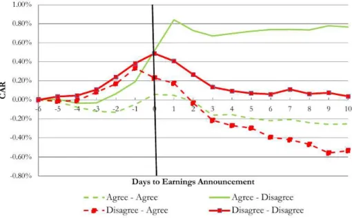
Figure 1: Abnormal returns when disagreement is or is not resolved after earnings announcement

Extracted from Giannini et al. [2013]. In they axis, CAR stands for cumulative abnormal return. The numbers on the x-axis represent the number of days since the earnings announcement was released. The graph shows that when disagreement is resolved (bottom-most line) the abnormal returns are the smallest. In contrast, when disagreement is created (top-most line), abnormal returns are the largest. “Abnormal” here stands for the fact that common factors explaning return have been “projected out”. The definition of “disagreement” in this context is whether the sign of the sentiment variable constructed with Twitter agrees with the sign of the measure constructed with news stories.

On the empirical side, the work that is closest in spirit to ours is the paper by Gi-annini et al. [2013]. They use sentiment analysis on Twitter and news stories to create a dummy variable indicating whether investors agree or disagree in a given point in time. With this measure, together with an earnings announcement, they test the ef-fect of the resolution of disagreement on abnormal returns, as summarized in Figure 1. Their focus, however, is not on testing whether earnings announcements tend to resolve disagreement. The measure of disagreement they construct could be useful for future work, maybe as a robustness check for the empirical analysis presented in this paper.

3

Methodology

Da et al. [2011] propose a measure for the attention allocated by investors to a stock, based on the volume of Google searches about the stock’s ticker (e.g., searches for AAPL as a measure of attention to Apple’s stock). They argue that their measure of attention have better properties than alternatives such as news coverage, extreme

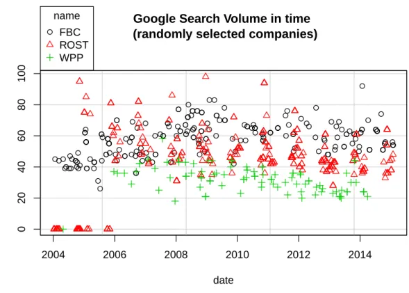
Figure 2: Google Search Volume in time for randomly selected companies

2004 2006 2008 2010 2012 2014

0 20 40 60 80 100

Google Search Volume in time (randomly selected companies)

date Search v olume ●●● ●●● ● ● ●●● ●● ● ●● ● ●● ● ● ● ● ● ● ●●●● ● ● ● ● ● ● ● ● ● ● ● ● ● ● ● ● ● ● ● ● ● ● ● ●● ● ● ● ● ● ● ● ● ● ● ●● ● ● ● ● ●● ● ● ● ●●● ● ●_● ● ● ● ● ● ● ● ● ●●●_●●● ● ● ● ●●● ● ● ● ● ● ● ● ●_●● ● ●● ● ● ● ● ● ● ● ●● ● ●● ● ● ● ● ● ● ● ● ● ● ●●●●●●● ● ●● ● ●● ● ●●●● ● ● ● ● ● ● ●● ● ●● ● ● ● ●_● ●● ● ●● ● ● ● ● ● ● ● ●● ● ● ● ● ● ● ● ● ●●● ● ● ● ● ● ● ●●●● ● ● ● ●●● ● ●_●●● ● name FBC ROST WPP

turns, and turnover. In fact, they find that their measure “leads alternative measures such as extreme returns and news, consistent with the notion that investors may start to pay attention to a stock in anticipation of a news event”. They also find that almost all of the time-series and cross-sectional variation in their measure is not accounted for by alternative proxies of attention, despite finding a positive correlation among them.

In this thesis, we use Google Trends to obtain data on the companies currently listed at the Russell 3000 index. Of about three thousand companies, 2029 have available weekly Google data. The other companies have only monthly data available, and are discarded from our sample. We illustrate Google data about three randomly selected companies on Figure 2.

The first thing to notice is that, in a given week, the search volume for a given term is a number between0and 100. This happens so that in the week where the greatest number of searches for a given term was made, the volume is 100; in all other weeks, volume is scaled so that it represents a percentage of the queries made in the week with most searches. Due to this scaling, the volume of Google searches is not comparable across companies, but only within companies. In other words, if (in a given week) companyXhas a volume of25and companyY has a volume of50, that doesnotmean that the number of Google searches forY is twice the number of Google searches for

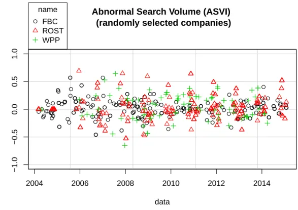
Figure 3: Abnormal Search Volume in time for randomly selected companies

2004 2006 2008 2010 2012 2014

−1.0

−0.5

0.0

0.5

1.0

Abnormal Search Volume (ASVI) (randomly selected companies)

data ASVI ● ● ●● ● ● ● ● ●● ●● ● ● ● ● ●● ● ● ● ● ● ●●●●● ● ● ● ● ● ● ● ● ● ● ● ● ●●● ● ● ● ● ●● ● ● ● ● ● ● ● ● ● ● ● ● ● ●●● ● ● ● ● ● ● ● ●● ●●●●●● ● ● ● ●● ● ● ● ●●● ● ●● ● ●● ●●● ● ●●● ● ● ● ●_●● ● ●● ● ● ● ● ● ● ● ●● ● ● ● ●● ● ● ● ● ●● ● ●●●●●●●●● ● ● ● ● ● ●●●●●● ● ● ●●● ● ● ●● ● ● ● ● ●● ●● ● ●● ● ● ● ● ● ● ● ●● ● ● ● ● ● ● ● ●● ●● ● ● ●●● ● ● ● ● ● ● ● ● ● ● ●● ●_●●● ● name FBC ROST WPP

Observation: Outliers have been omitted from this figure.

X.

The volume of Google searches for a term will be henceforth calledSearch Volume Index(SVI); in particular, the SVI of the stocki in timet will be denoted by SVIit. To

have a measure of attention that is comparable across companies, we transform the google data to obtain what we will callAbnormal Search Volume Index (ASVI).10 _{We do} so by evaluating the “log deviation” ofSV Iit with respect to the median of SV Iiτ in

the eight weeks prior tot. That is:

ASVIit = log(SVIit)−log (Median of SVIiτ during 8 weeks prior tot)

The ASVI for the same companies shown on Figure 2 can be seen on Figure 3. The summary statistics of SVI and ASVI comprising all companies are reported on Table 1. The data has been winsorized.

We now turn to the disagreement data. Remember that we want to assess the im-pact of greater investor attention on marketwide disagreement. As a measure of dis-10_{In adopting the names SVI and ASVI, as well as the formula for ASVI, we are following Da et al.}

[2011].

Table 1: Summary statistics - SVI and ASVI

Statistic N† _{Mean St. Dev. Min Max}

SVI 422,211 35.741 23.676 0 100

ASVI 419,383 0.028 0.556 −3.500 3.500

†The number of companies times the number of available days per company

agreement about a stock, we are going to used the standard deviation of analyst fore-casts about companies’ earnings-per-share (EPS hereinafter) in the I/B/E/S database. This is a standard measure in the empirical finance literature.11

The I/B/E/S database collects forecasts from hundreds of financial analysts. One typical entry in the database has 4 values that are relevant to us: the name of the ana-lyst, the date of the forecast, the company name and the forecast horizon. For example: analyst John, on Jan. 8, 2004, estimates that “Ross Stores Inc” will end up 2005 with an EPS of0.8. Analyst Jane, on the other hand, on Jan. 15, 2004, estimates that “Ross Stores Inc” will end up 2004 with an EPS of0.74. We say, in this case, that John’s forecast has a two-year horizon, and that Jane’s forecast has a one-year horizon. Since these are forecasts about the value in the end of the year, we adopt the date September 30th as the end of the fiscal year. So, in practice, we are assuming that John forecasts an EPS of 0.8on September 30th 2005, and Jane forecasts an EPS of0.74on September 30th 2004. We will henceforth call that date the “forecast horizon”.

From these individual analysts data, I/B/E/S forms a database of the standard deviation and mean of forecasts in given periods. We get two databases: one of them with one-year horizon forecast dispersions and means, another with two-year horizon forecast dispersions and means. One relevant problem with I/B/E/S data is that the standard deviation and mean of analyst forecasts is not updated in the database in frequent intervals. Rather, they are unevenly distributed in time, and the frequencies are different accross companies.

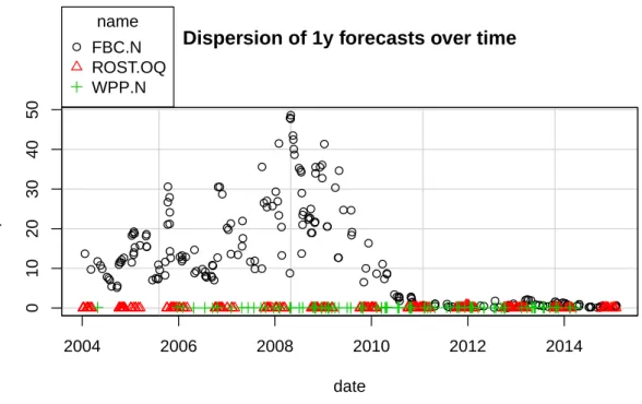
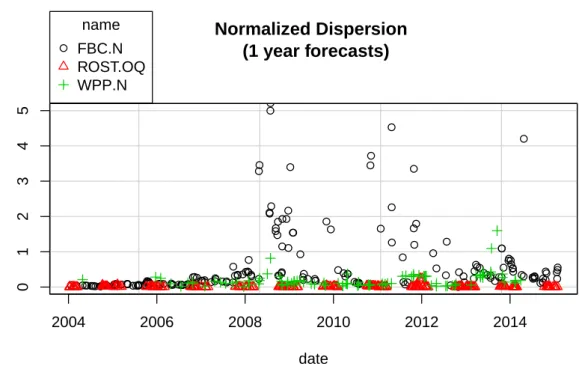
We define DISPitto be the standard deviation of analysts forecasts about company i on day t. We illustrate dispersion data in Figures 4 and 5, for one and two-year forecast horizons respectively. Notice the an enormous difference in magnitude across companies. To have interpretable coefficients in the regressions to come, we will divide the dispersions by the mean forecasts in absolute value (hence using what is commonly called the “relative standard deviation”) to form the NDISPit measure. We also use

the same transformation we applied above (on SVI) to create a measure of abnormal 11_{For a detailed discussion about its merits as a disagreement measure, we refer to the paper by}

Diether et al. [2002].

Figure 4: Dispersion of one-year horizon forecasts over time

2004 2006 2008 2010 2012 2014

0 10 20 30 40 50

Dispersion of 1y forecasts over time

date Dispersion _● ●●●● ●●● ●●● ●●●●●● ●● ● ● ●● ●● ●● ● ● ●●●● ●_● ● ● ● ● ● ● ● ● ● ● ●_●●_●●● ●●●●_●● ●●● ●● ● ● ●● ● ●●● ●●● ● ● ●● ●● ● ●● ●● ● ● ● ● ● ● ● ● ● ● ●_● ●_● ●●● ● ● ● ●●_●●●● ●●● ● ● ●●● ● ● ● ● ● ● ● ● ●● ● ● ● ● ● ●●_●●● ●_●●●●_{● ●}●●_{●● ●} ● ●●● ●●●●●●●● ●●● ●●●●●●●●●●●●●●●●●●●●●●●●●●●●●●● ●●●_{● ●●●●●●●●}●●●● ●●●● ● name FBC.N ROST.OQ WPP.N

Figure 5: Dispersion of one-year horizon forecasts over time

2004 2006 2008 2010 2012 2014

0

5000

10000

Dispersion of 2y forecasts over time

date Dispersion ● ● ● ●●● ● ● ● ● ● ● ● ● ● ●●● ● ● ● ● ● ● ● ● ● ●●_● ●_●● ●_● ● ●● ●_{●● ●} ● ● ● ● ● ● ● ● ● ●●●●●●_●● ● ●● ● ●●●●_●●● ● ● ● ● ● ● ● ●●●_{●●●●●}● ● ● ● ● ● ●● ● ●● ● ● ● ●● ● ●●● ● ● ●● ● ● ● ● ● ● ● ● ●●● ● name FBC.N WPP.N

Observation: The company “Ross Stores Inc” (ROST) is missing from the figure above because there weren’t two-year dispersions for it. This is probably due to the lack of forecasts on I/B/E/S, which

prevented the dispersion from being calculated.

Table 2: Summary Statistics - DISP, NDISP and ADISP - 1 year

Statistic N† _{Mean St. Dev. Pctl(25) Pctl(75) Min Max}

DISP 422,211 1.769 111.181 0.046 0.225 0.0003 15,816.940

NDISP 422,211 0.354 17.551 0.025 0.140 0.00002 10,000.000

ADISP 404,116 0.002 0.494 −0.160 0.123 −7.149 8.889

†The number of companies times the number of available days per company

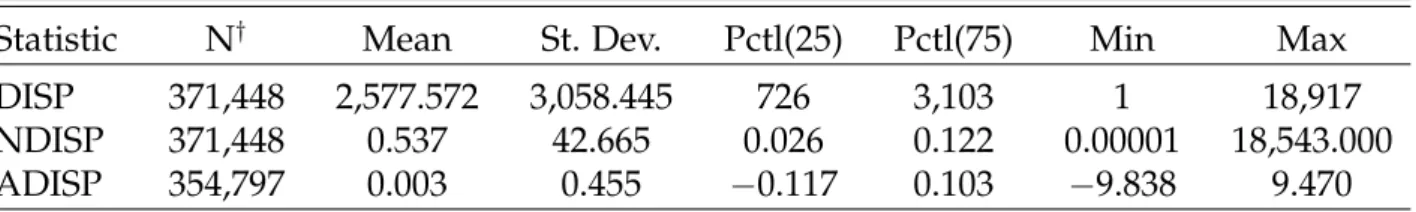
Table 3: Summary Statistics - DISP, NDISP and ADISP - 2 years

Statistic N† _{Mean St. Dev. Pctl(25) Pctl(75) Min Max}

DISP 371,448 2,577.572 3,058.445 726 3,103 1 18,917

NDISP 371,448 0.537 42.665 0.026 0.122 0.00001 18,543.000

ADISP 354,797 0.003 0.455 −0.117 0.103 −9.838 9.470

†The number of companies times the number of available days per company

dispersion, which we will call ADISP:

ADISPit= log(DISPit)−log (median of DISPiτ during 8 weeks prior tot)

that is, ADISPit is the log-deviation of the dispersion of forecasts with respect to the

median dispersion over the 8 weeks prior to t. Finally, we will call NDISPit the

dis-persion of forecasts normalized by their mean (in absolute value), that is, the “relative standard deviation” of forecasts. We have NDISP and ADISP plotted for three compa-nies in Figures 6 and 7. Finally, on Tables 2 and 3 we present summary statistics for DISP, ADISP and NDISP.

It seems to us that the best behaving measures of attention and dispersion, respec-tively, are ASVI and ADISP. For this reason, we will use them as our preferred measures of attention and disagreement in the exposition that follows. However, results using SVI and NDISP as measures (in logarithms) will also be reported. We conclude this section by discussing the regression strategy used for this thesis.

3.1

Regression strategy

In short, we assume a fixed effects model to estimate the following static panel.

ADISPhit =µi+βASVIit+Controls+ǫit (1)

where: the indexirepresents a company,tstands for time,h∈ {1,2}stands for forecast horizon. We run separate regressions forh = 1,2. ADISPitis theabnormaldispersion

Figure 6: Dispersion of one-year horizon forecasts over time

2004 2006 2008 2010 2012 2014

0 1 2 3 4 5 Normalized Dispersion (1 year forecasts)

date Nor maliz ed Dispersion ●●●●●●●●●●●●●●●●●●●●●●●●●●●●●●●●●●●●●●●●●●●●● ●●●●●●●●●●●●●●●●●●●●●●●●●●●●●●●●●● ● ●●●●●●● ● ● ●● ● ● ● ● ● ● ● ● ● ● ● ●●●● ● ●●● ● ● ● ● ● ● ●●●●●● ● ● ●●_●●● ●●●●●● ● ● ● ● ● ● ● ●●● ● ● ● ● ● ● ● ● ●●●●●●● ●●●●_{●●●●●} ●●● ● ● ●●●●●●● ● ●● ● ● ●●●●_●●●●●●● ●●● ● ● name FBC.N ROST.OQ WPP.N

Figure 7: Dispersion of one-year horizon forecasts over time

2004 2006 2008 2010 2012 2014

−2 0 2 4 6 Abnormal Dispersion (1 year forecasts)

date Abnor mal Dispersion ● ● ●_●●●●_●●● ●● ●_●●●_● ● ● ●_● ●●●●●● ● ●●●●●●● ● ● ● ● ● ● ●●● ●●● ●● ●●●●●●●●●_●● ●_● ● ●●●●● ●●_{● ●} ●● ● ●_{●●●●●●}● ● ● ● ● ●●●●●●●● ● ● ● ●●●●●●_●●●●●●●●●● ● ● ● ● ● ● ● ● ●●_● ●●● ●●●●●●●●● ●●● ●_● ●●●_●● _● ● ● ● ● ● ● ●● ● ●● ● ● ●_●●_● ● ● ● ● ●●●_●● ● ● ●● ● ● ●●●● ● ● ● ●● ● ● ● ● ● ● name FBC.N ROST.OQ WPP.N

Observation: Outliers have been omitted from Figure 6.

of forecasts of analysts about company i in period t, ASVIit is a measure of

abnor-mal attention allocated to companyi on time t. In all our regressions, we control for aggregate uncertainty by including the daily VIX index in the regressions. This is be-cause an underlying uncertainty might be causing simultaneously disagreement and a bigger number of google searches unrelated to the acquisition of information about companies. We don’t control for firm-specific uncertainty. We include a term which measures how close the forecast date is to the forecast horizon, to account for the fact that the forecast’s precision increases as the forecast horizon gets closer, and this has an obvious (negative) impact on disagreement.

In the following section, we report the regression results and interpret our find-ings. We leave the results of the regressions with NDISP as a dependent variable for Appendix B.

4

Results

We divide this section in three: first, we report results concerning the regressions based on one-year forecast horizons. Two-year forecasts horizons are left for subsection 4.2. We interpret the results and (attempt to) frame them in the literature in the last section.

4.1

One-year forecast horizon

On Table 4, the results of the regression of ADISP against ASVI as proposed in (1) are reported. In order to obtain a cleaner exposition, we did not report the coefficients of dummy variables corresponding to the years of the forecast dispersions. These dum-mies were included in all regressions.

With one-year horizon forecasts, we obtain the interesting result that greater atten-tion allocated to companies is (significantly) associated to greater disagreement about them. The significance and magnitude of this effect is not changed when aggregate uncertainty is accounted for.

We use the VIX index to control for aggregate uncertainty in two separate ways: first, we consider the sdVIX measure, which is simply the standardized VIX index; the interpretation of the sdVIX beta, therefore, is the impact on abnormal uncertainty of a one standard-deviation increase in the VIX index. An increase of one unit in abnormal uncertainty, in turn, can be interpreted as a one-percent increase in the dispersion of forecasts. We also consider the measure AVIX, which stands for abnormal VIX, and corresponds to the log deviation of VIX with respect to the median of VIX over the prior eight weeks.

The coefficient of the ASVI beta can be interpreted in the following way: a one standard deviation increase in ASVI about a company is associated to a 30 basis points increase in the dispersion of analyst forecasts. This is definitely a small magnitude, but in our view it is far from economically insignificant. Remember that our purpose is to understand the average response of disagreement about a company when more attention is allocated to it, and not to get the best possible linear fit. We defer a more detailed interpretation of the results to subsection .

While the coefficients on Table 4 are calculated under a homoskedasticity assump-tion, Table 5 shows that the coefficients of interested are still significant when het-eroskedasticity and autocorrelation within groups are accounted for. In this particular type of panel, calculating standard errors that are robust to correlation accross groups is a particularly complicated task, and we did not attempt to do so.12

4.2

Two-year forecast horizon

We reproduce everything that was done on subsection 4.1 with datbase of 2 year hori-zon forecasts. The results are reported on Table 6 in the exact same way. We find the disagreement of agents about a company on average does not respond to attention. This result loses its significance when possible heteroskedasticity and autocorrelation are taken into account, as shown in Table 7.

12_{Remember that the frequency of observations of analyst dispersion varies accross different}

compa-nies.

Table 4: Disagreement vs. Attention [1 year forecasts]

Dependent variable:

ADISP [dispersion]

(1) (2) (3) (4) (5)

ASVI [attention] 0.005∗∗∗ 0.005∗∗∗ 0.005∗∗∗ 0.005∗∗∗ 0.005∗∗∗ (0.001) (0.001) (0.001) (0.001) (0.001)

sdVIX [uncertainty] 0.047∗∗∗ 0.047∗∗∗ (0.001) (0.001)

ASVI*sdVIX [interaction] 0.002∗∗∗ (0.0005)

AVIX [uncertainty] 0.174∗∗∗ 0.173∗∗∗

(0.004) (0.004)

ASVI*AVIX [interaction] 0.008∗∗

(0.003)

Time until Forecast Horizon 0.001∗∗∗ _0.001∗∗∗ _0.001∗∗∗ _0.001∗∗∗ _0.001∗∗∗ (0.00001) (0.00001) (0.00001) (0.00001) (0.00001)

Observations 401,966 399,477 399,477 399,477 399,477 R2

0.043 0.047 0.047 0.047 0.047 Adjusted R2

0.043 0.047 0.047 0.047 0.047 F Statistic 1,397.8∗∗∗ 1,402.3∗∗∗ 1,310.1∗∗∗ 1,413.7∗∗∗ 1,319.9∗∗∗

(df = 13; 400234) (df = 14; 397744) (df = 15; 397743) (df = 14; 397744) (df = 15; 397743)

Note: ∗p<0.1;∗∗p<0.05;∗∗∗p<0.01

Table 5: Disagreement vs. Attention [1 year forecasts] – robust standard errors

Dependent variable:

ADISP [dispersion]

(Driscoll-Kraay) (Arellano) (Driscoll-Kraay) (Arellano) ASVI [attention] 0.005∗∗∗ _0.005∗∗∗ _0.005∗∗∗ _0.005∗∗∗

(0.001) (0.001) (0.001) (0.001)

sdVIX [uncertainty] 0.047∗∗∗ _0.047∗∗∗ (0.011) (0.002)

ASVI*sdVIX 0.002∗∗ _0.002∗∗∗ (0.001) (0.001)

AVIX [uncertainty] 0.173∗∗∗ _0.173∗∗∗ (0.051) (0.007)

ASVI*AVIX 0.008 0.008

(0.005) (0.006)

distanciaTempo 0.001∗∗∗ _0.001∗∗∗ _0.001∗∗∗ _0.001∗∗∗ (0.0001) (0.00002) (0.0001) (0.00002)

Observations 399,477 399,477 399,477 399,477

Note: ∗_p<0.1;∗∗_p<0.05;∗∗∗_p<0.01

It is interesting to notice that the magnitude of the sdVIX coefficient is less than half of what it was in the 1 year case; this indicates that forecasts about the performance of companies in the medium-run are less subject to “negative sentiment” driven by aggregate uncertainty.

For the sake of completeness, we include interaction terms in these regressions, even though they are insignificant when heteroskedasticity and autocorrelation are taken into account.

4.3

Interpretation of results

The idea that agents interpret the world through different economic models and thus more information can lead to disagreement between investors finds support in our results. This intuition is explored in several papers in what Hong and Stein [2007] call disagreement models, e.g. Harris and Raviv [1993], Kandel and Pearson [1995], and Kondor [2012] .

To be more specific, we find evidence that an increase in disagreement is associated to an increase in attention even after controlling for an increase in uncertainty at the economy. This result goes against the classical intuition that information tend to re-solve disagreement between investors.13 _{We have two possible interpretations of our} results. First, an increase at SVI means more people are learning about that company. With a bigger pool of possible investors there is also a wider variety of “economics models” through which the firm is being analised. This leads to a possibly larger level of disagreement between investors. Second, even if there is no increase in the number of investor analysing the company, more searches on Google means more information (about this firm) is being processed by investors. But even if investors are looking at the exact same new information, disparity in their “models” lead then to interpret it in distinct ways.

Now, our results do disappear for two-year horizon forecasts. We still don’t have a definitive explanation for that. The two-year data base is smaller than the one rel-ative to one-year forecasts. However, there is no reason to believe this data set is not big enough for our purposes. Despite that, this difference in size does bring a rele-vant question. Why don’t investors make (or send) to Reuters their predictions for 2 years ahead as frequently? What incentives do agents face when deciding to make predictions for future earnings-per-share? Do these incentives change for diferent time 13_{According to Miller [1977], the lack of information makes differences of opinion greater when an}

IPO occurs. As time passes, the company acquires a history of earnings and the market indicate how it will value these earnings. He argues that this should decrease uncertainty and disagreement between market participants.

horizons?

Table 6: Disagreement vs. Attention [2 year forecasts]

Dependent variable:

ADISP [abnormal dispersion]

(1) (2) (3) (4) (5)

ASVI [attention] 0.00000∗∗ 0.00000∗∗ 0.00000∗∗ 0.00000∗∗ 0.00000∗∗ (0.00000) (0.00000) (0.00000) (0.00000) (0.00000)

sdVIX [uncertainty] 0.021∗∗∗ 0.021∗∗∗ (0.001) (0.001)

ASVI*sdVIX −0.00000

(0.00000)

AVIX [uncertainty] 0.050∗∗∗ 0.045∗∗∗

(0.004) (0.006)

ASVI8*AVIX 0.00000

(0.00000)

distanciaTempo 0.0004∗∗∗ _0.0004∗∗∗ _0.0004∗∗∗ _0.0004∗∗∗ _0.0004∗∗∗ (0.00001) (0.00001) (0.00001) (0.00001) (0.00001)

Observations 352,875 350,849 350,849 350,849 350,849 R2

0.008 0.009 0.009 0.009 0.009

Adjusted R2

0.008 0.009 0.009 0.009 0.009

F Statistic 247.524∗∗∗ 248.138∗∗∗ 230.419∗∗∗ 236.091∗∗∗ 219.325∗∗∗ (df = 12; 351162) (df = 13; 349135) (df = 14; 349134) (df = 13; 349135) (df = 14; 349134)

Note: ∗p<0.1;∗∗p<0.05;∗∗∗p<0.01

Table 7: Disagreement vs. Attention [2 year forecasts] – robust standard errors Dependent variable:

ADISP

(Driscoll-Kraay) (Arellano) (Driscoll-Kraay) (Arellano)

ASVI [attention] 0.00000∗ _{0.00000 0.00000}∗ _0.00000

(0.00000) (0.00000) (0.00000) (0.00000)

sdVIX [uncertainty] 0.021∗∗∗ _0.021∗∗∗

(0.004) (0.002)

ASVI*sdVIX −0.00000 −0.00000

(0.00000) (0.00000)

AVIX [uncertainty] 0.045∗∗ _0.045∗∗∗

(0.019) (0.010)

ASVI*AVIX 0.00000 0.00000

(0.00000) (0.00000)

distanciaTempo 0.0004∗∗∗ _0.0004∗∗∗ _0.0004∗∗∗ _0.0004∗∗∗

(0.00003) (0.00002) (0.00003) (0.00002)

Observations 350,849 350,849 350,849 350,849

Note: ∗_p<0.1;∗∗_p<0.05;∗∗∗_p<0.01

First of all, Thomson Reuters keeps a ranking of analyst-accuracy. This information is used to calculate “StarMine SmartEstimates”, a Thomson Reuters product which is basically a weighted average of investors estimates. It seems reasonable that giving more weight to estimates made by best ranked analysts will create a better predictor. Also, when an analyst is fired, he carries with him this analyst-accuracy score. Addi-tionally, some banks calculate bonus payments based on analyst performance provided by Reuters.14 _{Because of that, investors are willing to send their estimates to Reuters.} Maybe there is a key difference in incentives for sending estimates for current and future fiscal year, further investigation is needed. Maybe analyst wait longer before updating long run estimates. If this is the case, the predictions for current fiscal year represent investors opinion in a more timely manner and thus are more suited for this thesis goals.

There is also the possibility that ASVI is an endogenous component in model (1). For example, as already mentioned, a firm-specific “uncertainty shock” in a period could be causing agents (possibly even outside of the financial markets) to allocate at-tention to the stock, and simultaneously causing short term disagreement to increase. Since longer term forecasts are possibly less subject to investor sentiment, this would explain why the dispersion in two-year horizon forecasts does not show the same re-lationship with attention as the one-year forecasts. To investigate if this is actually the case, one possible line of investigation would be to use a vector autoregression approach to determine if disagreement leads increases in attention (or the other way around). Also, one could use an instrumental variable framework to analyse if purely exogenous variations in attention are associated to bigger disagreement. In any case, we consider this a natural path for future research.

5

Conclusion

We evaluate the impact of a novel measure of attention proposed by Da et al. [2011] on marketwide disagreement, as measured by the dispersion of analyst forecasts. The attention measure is based on the volume Google searches for companies’ tickers (e.g., AAPL for Apple). We find that when agents allocate more attention to a company, disagreement about it increases. In other words, when agents are looking at firm-specific information, they tend to disagree more, even when aggregate uncertainty is controlled for. We interpret this as adding evidence to the “differential interpretation” models proposed by Harris and Raviv [1993] and Kandel and Pearson [1995].

14_{This information is the result was provided by a seller of Thomson Reuters products. We have not}

yet confirmed to what extent this is true.

References

Laurence Ball, N Gregory Mankiw, and Ricardo Reis. Monetary policy for inattentive economies. Journal of monetary economics, 52(4):703–725, 2005.

Andrea Buraschi and Alexei Jiltsov. Model uncertainty and option markets with het-erogeneous beliefs. The Journal of Finance, 61(6):2841–2897, 2006.

Andrea Buraschi, Fabio Trojani, and Andrea Vedolin. When uncertainty blows in the orchard: Comovement and equilibrium volatility risk premia. The Journal of Finance, 69(1):101–137, 2014.

Zhi Da, Joseph Engelberg, and Pengjie Gao. In search of attention. The Journal of Finance, 66(5):1461–1499, 2011.

Karl B Diether, Christopher J Malloy, and Anna Scherbina. Differences of opinion and the cross section of stock returns. The Journal of Finance, 57(5):2113–2141, 2002.

Robert Charles Giannini, Paul J Irvine, and Tao Shu. The convergence and divergence of investors’ opinions around earnings news: Evidence from a social network. Work-ing paper, 2013.

Milton Harris and Artur Raviv. Differences of opinion make a horse race. Review of Financial studies, 6(3):473–506, 1993.

J Michael Harrison and David M Kreps. Speculative investor behavior in a stock mar-ket with heterogeneous expectations. The Quarterly Journal of Economics, pages 323– 336, 1978.

Marek Hlavac. stargazer: LaTeX/HTML code and ASCII text for well-formatted regression and summary statistics tables. Harvard University, Cambridge, USA, 2014. URLhttp: //CRAN.R-project.org/package=stargazer. R package version 5.1.

Harrison Hong and Jeremy C Stein. Disagreement and the stock market (digest sum-mary). Journal of Economic perspectives, 21(2):109–128, 2007.

Harrison Hong, Jeremy C Stein, and Jialin Yu. Simple forecasts and paradigm shifts. The Journal of Finance, 62(3):1207–1242, 2007.

Eugene Kandel and Neil D Pearson. Differential interpretation of public signals and trade in speculative markets. Journal of Political Economy, pages 831–872, 1995.

Péter Kondor. The more we know about the fundamental, the less we agree on the price. The Review of Economic Studies, 79(3):1175–1207, 2012.

Edward M Miller. Risk, uncertainty, and divergence of opinion. The Journal of Finance, 32(4):1151–1168, 1977.

Lin Peng and Wei Xiong. Investor attention, overconfidence and category learning. Journal of Financial Economics, 80(3):563–602, 2006.

Ricardo Reis. Inattentive consumers. Journal of monetary Economics, 53(8):1761–1800, 2006a.

Ricardo Reis. Inattentive producers. The Review of Economic Studies, 73(3):793–821, 2006b.

Christopher A Sims. Stickiness. InCarnegie-Rochester Conference Series on Public Policy, volume 49, pages 317–356. Elsevier, 1998.

Christopher A Sims. Rational inattention: Beyond the linear-quadratic case. The Amer-ican economic review, pages 158–163, 2006.

Michael Woodford. Imperfect common knowledge and the effects of monetary policy. Technical report, National Bureau of Economic Research, 2001.

Appendix

A

Simple example of greater disagreement upon

obser-vation of a public signal

Two bayesian learners,i and j, are interested in an unobserved parameter θ ∈ Θ :=

{θ, θ}. They have (proper) priors(πi_{, π}i_)and(πj_{, π}j_)onΘ.

They observe a random signals∈ Σ :={σ, σ}whose true distribution depends on

θ. The (true) probability of observing signalσ∈Σgiven someθis denoted by

Pr(s=σ|θ)

If an agent knew the probability measure above, by observing a sequence of iid realizations of s she could (by the law of large numbers) learn the true parameter θ. However, the conditional probability above is unknown to bothiandj. They use their own estimate of the conditional probability, which we denote by

Prk(s=σ|θ) k ∈ {i, j},

to learn about the parameter θ. We say that the above conditional probability is agentk’s interpretation, or economic model of the environment. In this setting, we say that they havedifferences of opinion when the conditional probabilities are different for

iandj.

With these probability measures, after observing a realization s = σ of the signal, they update their beliefs according to Bayes’ rule:

Prk_{(θ=θ|s=σ) =} Pr

k_{(s =σ|θ)Pr}k_(θ=θ)

Prk(θ=θ)P r(s=σ|θ =θ) + Prk(θ=θ)Prk(s=σ|θ =θ)

= π

k_Prk

(s =σ|θ)

πk_{P r(s=σ|θ =θ) +π}k_Prk

(s =σ|θ=θ)

= 1

πk πk

Prk(s =σ|θ =θ) Prk_{(s =σ|θ =θ)} + 1

To simplify notation, we denote the ratioπk_/πk _asrk

0 andPr

k

(s =σ|θ =θ)/Prk(s=

σ|θ =θ)asrk

1. This way, we write

Prk_{(θ=θ|s=σ) =} 1

1 +rk

0rk1

We interpretrk

0 as an “initial likelihood ratio”, and r1k as the likelihood ratio after ob-servings=σ(both, of course, from agentk’s perspective).

A measure of the disagreement between agents afterobserving the signal is given by

Pr

i_{(θ=θ|s=σ)−Pr}j_{(θ =θ|s=σ)}

=

|rj0(r

j

1−r1i) +ri1(r

j

0−ri0)|

(1 +ri

0ri1)

1 +rj0r

j

1

One first intersting thing to notice is that, if agents have the same priors (in which caser0j = r

j

1), but interpret the signal differently, then they necessarily disagree after observing the signal. The level of the resulting disagreement, however, depends on the ratiosri

1andr

j

1. If both ratios are large, the agents interpret the signal as providing evidence that the true θ is notθ¯. In this case, their level of disagreement, in spite of being positive, is small. Finally, whether or not they end up disagreeing in the case of different prior beliefs depends on the signals and relative magnitudes of (r1j −r1i)/ri1 and(r0j−r0i)/ri0.

B

Results of secondary regressions

As mentioned earlier, we also run regressions based on NDISP and SVI. These regres-sions have the form

log (NDISPit) =µi+βlog (SVIit) +Controls+ǫit (2)

The results are on Table 8 on the next page.

Table 8: DISP vs. SVI, one and two year forecasts

Dependent variable:

log(NDISP)

(1) (2) (3) (4)

log(SVI) 0.012∗∗∗ 0.012∗∗∗ 0.010∗∗∗ 0.010∗∗∗ (0.001) (0.004) (0.001) (0.003)

sdVIX −0.042∗∗∗ −0.042∗∗∗ −0.037∗∗∗ −0.037∗∗∗ (0.009) (0.012) (0.008) (0.011)

Time until Forecast Horizon 0.002∗∗∗ 0.002∗∗∗ 0.0005∗∗∗ 0.0005∗∗∗ (0.00004) (0.00004) (0.00004) (0.00004)

sdVIX:SVI 0.0003∗∗∗ 0.0003 0.001∗∗∗ 0.001∗∗ (0.0001) (0.0003) (0.0001) (0.0003)

Observations 419,649 419,649 369,330 369,330 R2

0.132 0.132 0.082 0.082

Adjusted R2

0.131 0.131 0.081 0.081

F Statistic 4,225.257∗∗∗ 4,225.257∗∗∗ 2,336.989∗∗∗ 2,336.989∗∗∗ (df = 15; 417911) (df = 15; 417911) (df = 14; 367600) (df = 14; 367600)

Note: ∗p<0.1;∗∗p<0.05;∗∗∗p<0.01