Mechanics and dynamics of X-chromosome pairing at X inactivation.

Inactivation

Antonio Scialdone1,2, Mario Nicodemi2,3*

1Dipartimento di Scienze Fisiche, Universita` di Napoli ‘‘Federico II’’, Naples, Italy,2INFN, Naples, Italy,3Department of Physics and Complexity Science, University of Warwick, Coventry, United Kingdom

Abstract

At the onset of X-chromosome inactivation, the vital process whereby female mammalian cells equalize X products with respect to males, the X chromosomes are colocalized along their Xic (X-inactivation center) regions. The mechanism inducing recognition and pairing of the X’s remains, though, elusive. Starting from recent discoveries on the molecular factors and on the DNA sequences (the so-called ‘‘pairing sites’’) involved, we dissect the mechanical basis of Xic colocalization by using a statistical physics model. We show that soluble DNA-specific binding molecules, such as those experimentally identified, can be indeed sufficient to induce the spontaneous colocalization of the homologous chromosomes but only when their concentration, or chemical affinity, rises above a threshold value as a consequence of a thermodynamic phase transition. We derive the likelihood of pairing and its probability distribution. Chromosome dynamics has two stages: an initial independent Brownian diffusion followed, after a characteristic time scale, by recognition and pairing. Finally, we investigate the effects of DNA deletion/insertions in the region of pairing sites and compare model predictions to available experimental data.

Citation:Scialdone A, Nicodemi M (2008) Mechanics and Dynamics of X-Chromosome Pairing at X Inactivation. PLoS Comput Biol 4(12): e1000244. doi:10.1371/ journal.pcbi.1000244

Editor:Gary D. Stormo, Washington University, United States of America

ReceivedJune 2, 2008;AcceptedNovember 6, 2008;PublishedDecember 26, 2008

Copyright:ß2008 Scialdone, Nicodemi. This is an open-access article distributed under the terms of the Creative Commons Attribution License, which permits unrestricted use, distribution, and reproduction in any medium, provided the original author and source are credited.

Funding:No funding was received for this work.

Competing Interests:The authors have declared that no competing interests exist. * E-mail: mario.nicodemi@na.infn.it

Introduction

In female mammalian cells one X chromosome has to be inactivated in order to equalize the dosage of X genes products with respect to males [1–3]. Such a phenomenon, known as X-chromosome inactivation (XCI), is regulated by a long region of the X, theX Inactivation Center(Xic). A crucial initial step that occurs during XCI is the physical colocalization of the two Xic’s [4–6]. Disruptions of pairing induce XCI failure and cell death, yet the mechanisms whereby the two Xic’s recognize each other and colocalize remain obscure.

In murine embryonic stem cells, pairing occurs within the early days of differentiation. Two major regions of colocalization have been discovered (see Figure 1): a sequence betweenTsixand Xite

genes, close to [4,5]; and a segment located several hundred kilobases upstream, named Xpr [6], colocalizing independently fromTsix/Xite. While the specific role of these regions is still under investigation, several details ofTsix/Xitehave been elucidated.

Its colocalization requires some few kilobase long DNA subfragments and a known Zn-finger protein, CTCF, having several DNA binding domains which can bind those subfragments at multiple and clustered sites [4,7] (see Figure 1). Since the inhibition of transcription ofTsixandXitedisrupts the formation of X–X couples, it has been, thus, proposed that the X chromosome interaction is mediated by a transiently stable ‘‘RNA-protein bridge’’ at these specificXicsites [7].

Importantly, the insertion on autosomes (non sex chromosomes) of the mentioned Tsix/Xite and Xpr segments ofXic induces X-autosome pairing [4,6,7]. A still unexplained result is that

deletion/insertions, including pairing regions, affect the strength of pairing according to their length, e.g., longer heterozygous deletions exhibit weaker pairing, as in the case of XXDXite and

XXDTsixentailing the removal of 3.7 and 5.6 kbps respectively [4]. Consistently, longer insertions of Xic pairing segments produce stronger X-autosome pairing; and, in females, X-autosome interactions compete with X–X pairing [4]. As deletions of those DNA regions and mutations of CTCF disrupt colocalization, these elements are thought to be necessary components of the pairing machinery. The crucial questions, though, on whether they are sufficient, on the mechanical basis and the physical requirements producing X chromosomes recognition, colocalization and time orchestration, are still unanswered.

To this aim, we investigate a schematic physics model of the molecular elements involved in the pairing of these loci, which includes the general features of DNA sequences (e.g.,Tsix/Xite

subfragments) and molecular factors (e.g., CTCF) summarized above. By extensive computer simulations, we show that Xic

regions can be, indeed, spontaneously colocalized as the result of their interaction with binding soluble molecular factors. Thermo-dynamics imposes, however, that Xic’s do recognize each other and come into physical proximity only if mediator concentration, or their affinity, exceeds a critical value, else they move independently. This grounds on Statistical Mechanics the proposed ‘‘RNA-protein’’ bridge scenario of colocalization [7], by disclosing its physical requirements, it suggests how the cell can regulate it. The model also predicts the kinetics and probability of

insertions into the X pairing sequences, as much as of chemical modifications of DNA and molecular factors (e.g., CTCF) are investigated.

Results

The Model

Since the molecular components of the ‘‘RNA-protein bridge’’ and their DNA binding sites are only partially known (e.g., CTCF and itsTsix/Xitebinding sites), we consider here a general model, which can accommodate other elements, aiming to depict a broader scenario. In our physics model, the two Xic segments involved in the process are represented as two directed polymers of

nbeads (see Figure 2 and Methods), a well established model of polymer physics [8], while, for sake of simplicity, the rest of the X chromosomes is neglected. Along the polymers, a subset of beads acts as binding sites (BSs, green beads in Figure 2) for molecular

are likely to have different chemical affinities in reality, nevertheless, we suppose they are all equal to an average value,

E, and we mostly focus on the case whereEis in the range of weak biochemical energies, as expected from the CTCF example. MFs and the two DNA segments float in a box of given size (see Figure 2 and Methods). By extensive Monte Carlo computer simulations [10], the thermodynamics and, later, the dynamics of the system are investigated.

Chromosome Spontaneous Colocalization

The ‘pairing state’of the Xic segments is monitored by measuring the average fraction, p, of colocalized Xic’s, i.e., the fraction of couples whose equilibrium mean distance is less than 10% of the linear size of the including volume.

In presence of a given concentration,c, of MFs a bridge between the two polymers could be formed by chance when a MF binds both simultaneously. As a single bridging event is statistically unlikely and short lived, the degree of pairing between theXic’s is expected to be stronger the higher c. However, a threshold behaviour exists. Figure 3 shows the thermodynamic equilibrium value of p as function of c (for E= 1.2kT): below a threshold,

c*

.2.3% (defined by the inflection point of p(c)), pis practically zero irrespective ofc. Such a region is the ‘Brownian phase’ where molecules are unable to form thermodynamically stable bridges and chromosomes move independently (a typical configuration is depicted in Figure 2A). Conversely, if c is above threshold, p

rapidly approaches 100%, signaling the transition to a different regime, the ‘pairing phase’: here chromosomes have spontane-ously, and ineluctably, recognized and paired by the effects of a stable effective attraction induced by MFs (a configuration is shown in Figure 2C). The colocalization process is, though, fully

quantitative model, from statistical mechanics, which elucidates the mechanical basis of such phenomena. We demonstrate that a set of soluble molecules binding specific DNA sequences are sufficient to induce recogni-tion and colocalizarecogni-tion. This is possible, however, only when their binding energy/concentration exceeds a threshold value, and this suggests how the cell could regulate colocalization. The pairing mechanism that we propose is grounded in general thermodynamic principles, so it could apply to other DNA pairing processes. While we also explore the kinetics of X colocalization, we compare our results to available experimental data and produce testable predictions.

Figure 1. Diagram of theXicregion involved in X chromosome pairing.The location ofXpr[6] andTsix/Xite[4,5], the regions involved in pairing at the onset of X-Chromosome Inactivation (XCI), is mapped within the X-Inactivation center (Xic). The red line with arrows highlights the area whereXprhas been localized [6]. The enlargement of theTsix/Xiteregion reports the discovered binding sites for CTCF [7].

reversible by reduction of MF concentration below threshold. Around c*, a narrow crossover region exists between these two phases wherep(c) is significantly different from zero, but still well below 100%, as couples of chromosomes are continuosly formed and disrupted (see the configuration in Figure 2B). In the thermodynamic limit (i.e., for an infinitely large system), the inflection point,c*, corresponds to a phase transition. For a finite sized system, as the one simulated here, p(c) is well fitted by an exponential:

p cð Þ~1{exph{ðc=c0Þbi

wherebis a fitting parameter (for the case discussed in Figure 3, we findb= 4.7) andc0is proportional to the threshold value,c*,

found above c~c0 b{1

b 1=b

.

For a given value ofc, the route to colocalization could be taken, analogously, by increasing E, as a result, for instance, of modifications of the DNA binding regions or of mediating molecular complexes. Under this different path, a threshold exists as well, as summarized in the phase diagram of Figure 4, showing the equilibrium pairing state of the Xic’s in the concentration-energy plane, (c,E), along with the transition line,c*(E), between the two phases. The existence of the threshold line,c*(E), has its roots in a thermodynamic phase transition occurring in the system, where the energy gain resulting from pairing compensates the corresponding entropy loss [11]. In particular, we find a power law behavior for the functionc*(E) at smallE(superimposed fit):

cð ÞE *ðE{EminÞ {n

where the exponent is n,4, and Emin.0.7kT is a minimal threshold energy below which no pairing transition is possible. At higher E an exponential fit of c*(E) works as well. The phase diagram of Figure 4 gives precise constraints to the admissible

Figure 3. Equilibrium state as function ofc.The equilibrium value of the fraction of paired chromosomes,p, is plotted as function of the concentration,c, of binding molecular factors, for a given value of their affinity,E(here,E= 1.2kT). When the concentration is below a threshold value c*.2.3%, no stable pairing is observed (p,0) and the chromosomes randomly float away from each other (‘Brownian phase’). Above threshold,psaturates to 100%, as a phase transition occurs (to the ‘Pairing phase’) and chromosomes spontaneously colocalize, their driving force being an effective attraction of thermodynamics origin. doi:10.1371/journal.pcbi.1000244.g003

Figure 4. Phase diagram.The diagram shows the thermodynamic equilibrium state of the system in the (E,c) plane, for a range of typical biochemical binding energies,E, and concentrations,c. Circles mark the line c*(E) delimiting the transition from the Brownian phase, where chromosomes diffuse independently, to the Pairing phase, where chromosomes are juxtaposed (the superimposed fit is a power law). doi:10.1371/journal.pcbi.1000244.g004

Figure 2. Typical equilibrium configurations.Pictures of typical configurations of our model system at thermodynamic equilibrium (here

E= 1.2kT). (A) Polymers conformation for a value of the concentration of molecular factors (MFs)c= 0.3% (Brownian phase, see Figure 4), (B) for

values of c and E to attain colocalization. On the other hand, colocalization is found in a broad range of weak biochemical binding energies and concentrations, pointing out that the recognition/pairing mechanism here envisaged is robust, irrespec-tive of the ultimate biochemical details of the ‘‘RNA-protein bridge’’ and its binding sites.

The Dynamics of Colocalization

To analyze the system dynamics, in our simulations MFs are initially randomly distributed in the enclosing volume and the two DNA segments start from the maximal possible distance from each other, so, at timet= 0 the pairing fraction isp= 0. Figure 5 reports

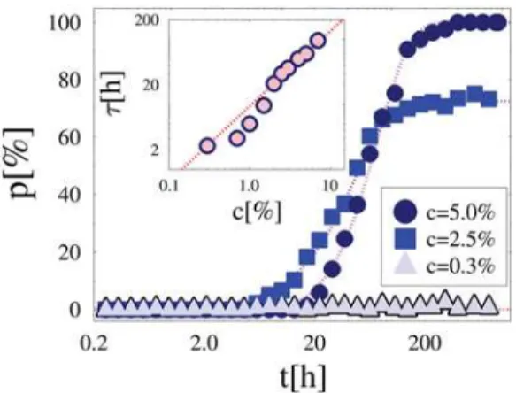
p(t), i.e., the change in time of p, for three values of the concentration which belong to the different regimes discussed above (here,E= 1.2kT). For c= 0.3%, i.e., below threshold,p(t) never rises above the background zero value. By increasingc to

c= 2.5% and 5%, close to and above the threshold, chromosomes ‘‘sense’’ each other [6], as p(t) grows to its non-zero equilibrium value,p(c), seen before. After an initial Brownian regime, where

p(t)/t, at long times an exponential dynamics is recorded (superimposed fit in Figure 5):

p tð Þ_^p cð Þ 1{e{t=t

wherep(c) is the equilibrium value discussed above. The parameter

t, a function ofcandE, is a measure of the average time to attain equilibrium (and pairing forc.c*) [Note: a full fit function forp(t)

is:p tð Þ~p cð Þ{ p cð Þz₁c:t zd:t

h i

e{t=t_{, wherecandd(such ast) are}

fit parameters depending on the values ofc andE. This fits our data very well, however, we prefer to report the simpler one-parameter exponential fit which is sufficient to estimate the characteristic time scale, t. The two fits provide approximately equal values oft].

Interestingly, tincreases when the number of MFs increases, approximately linearly inc(see inset Figure 5 and superimposed

also because other phenomena may affect the kinetics of chromosomes. Nevertheless, a dependence of the diffusion constant on the molecular factor concentration should be observed locally, at the scale of the pairing sequences.

The Distribution of Chromosome Distance

Further insight and direct comparisons to known experimental results [4–6] are obtained by studying the dynamics of the probability distribution, F, of the normalized distance, ND, between the X chromosomes (ND is normalized by the system volume linear size, so 0,ND#1). In these simulations, the two DNA segments are initially randomly scattered across the lattice, as much as the MFs. The typical shape of the functionFðNDÞ, in the region where pairing occurs, is reported in Figure 6A, at two time frames. Att= 0, F has the same shape, and approximately the same mean value, of the normalizedXicdistance distribution measured in mouse embryonic stem cells at the beginning of differentiation ([4] and inset of Figure 6A). In mice, Tsix/Xite

pairing is observed approximately within day two from differen-tiation [4–7]. In our simulations, a peak inFðNDv₀:₁Þ_{grows in} time and after around 48 h saturates to its final value (forc= 5% andE= 1kT). The final distribution is bimodal: superimposed to the peak inFðNDv₀:₁Þ_{, which corresponds to the chromosomes} bridged by MFs, there is a much broader distribution (very similar to the initial random one, with a peak approximately centered in

ND.0.5) which corresponds to independently floating chromo-somes. The cumulative frequency distribution of chromosomes with ND below 0.1, i.e., ‘paired chromosomes’, plotted in Figure 6B, shows the growth of the component of bridged chromosomes in the statistical population. The overall shape of the distribution, FðNDÞ, and its change with time, found in our simulations reproduce qualitatively very well those observed in the experiments (see inset of Figure 6A). This is intriguing when considering the simplicity of our model and the fact that we use just simple reasonable guess values for binding energy, E, and kinetic constant,r0(which have still to be experimentally found). A

number of further complexities are present in real experiments (e.g., averages over non uniform populations of cells, difficulties in resolving neighboring fluorescent spots, etc.), which could explain discrepancies in the details.

To estimate the fraction of pairing events in a given time window, it is also important to calculate the distribution of ‘collision’times: we measured the time, tcollision, needed by a

chromosome to encounter for the first time the other, i.e., to be located within a normalized distance,ND, less than 0.1 from it; Figure 6C illustrates the probability distribution,P, oftcollision(for

the same parameter values of Figure 6A and 6B). Note thattcollision

is the time for just a ‘collision’to occur, which could either result in a stable pairing or not.P is approximately exponential intcollision:

PðtcollisionÞ~P0expð{tcollision=t0Þ

Figure 5. System Dynamics. The average fraction of paired chromosomes,p, is plotted as a function of time,t, for three values of the concentration of molecular factors,c(hereE= 1.2kT), belonging to three different regimes: Brownian c= 0.3%; crossover c= 2.5%; Pairingc= 5%. After an initial diffusive behavior, chromosomes attain their equilibrium pairing state exponentially in time (superimposed fit:

p(t)/[12exp(2t/t)]). Inset: The average time scale, t, to attain the equilibrium pairing state is plotted as function ofc(forE= 1.2kT).t

P0andt0being fit parameters (for the case in Figure 6C we find

P0~31:5%andt0= 30h).

Heterozygous Deletions

Finally, we also explored the effects on pairing of heterozygous deletions, an issue of practical relevance to experimental studies. We consider the case where the BSs on oneXicare reduced to a fraction, f, of their original number n0 (for the same MF

concentration, c= 5%, and affinity E= 1.2kT, mostly discussed before). While a reduction of the pairing fraction,p, is expected in presence of a deletion, we find that the equilibrium value ofphas a non-linear behavior inf, a sigmoid with a threshold atf*,50% (see Figure 7): short deletions (say, preserving a fraction of BSsf$70%) do not result in a relevant reduction of p, while pairing is completely lost as soon as f gets smaller than about 30%. The sigmoid behavior stems from the non trivial thermodynamic origin of the MF mediated effective attraction between Xic’s. The threshold value, f*, is a decreasing function of E and c. While similar considerations to those mentioned when discussing p(c) apply, we find that an exponential fits p(f) (superimposed line in Figure 7):p(f) = 12exp[2(f/fp)

l

], wherelis a fitting parameter (for

the case discussed in Figure 7, we find l= 4.2) and fp is

proportional to the threshold f* discussed above f~fp l{l1

1=l

. While these results rationalize the observed length dependent effects ofTsix/Xitedeletions [4], the predicted behavior ofp(f) could be experimentally tested.

Interestingly, the time to approach the equilibrium state,t, is smaller the longer the deletion, as shown in the inset of Figure 7. Such a seemingly counterintuitive result stems from the fact that the smallerf, the smaller is the number of MFs attached to Xic segments and, thus, larger their effective diffusion constant (see above). The function t(f) is well fitted by: tð Þf ~ tð Þ0z_Dt1{e{ðf=ftÞg_{; for the case shown in the inset of} Figure 7, the fit parameters are t(0) = 3.6h, Dt= 56.4h,

ft= 59% and g= 3.5, but they are functions of E and c (as discussed above). The increasing behaviour oftas function off

results in a non-trivial prediction: the removal of a fraction of BSs within a chromosome should speedXicpairing with respect to the Wild Type case, although, the overall fraction of paired chromosomes would be reduced. As seen in the inset of Figure 5, an analogous phenomenon would be observed by decreasing the concentration of MFs.

Figure 6. Distance and collision times distribution.(A) The distributionF of the normalized distance,ND(0,ND#1), between the two X chromosomes is plotted at two time frames (in the phase where pairing occurs, herec= 5%,E= 1kT). The initial distribution corresponds to randomly located chromosome positions (t= 0 h); while colocalization progresses a peak inFðNDv_0:1Þbecomes visible and saturates at 48 h. In the inset the

corresponding experimental data (from [4]) are reported. (B) The cumulative frequency distribution of ‘paired chromosomes’(i.e., havingND,0.1), under the same conditions of (A), is shown. (C) Probability distributionPof the timetcollisionrequired by a chromosome to encounter for the first time the other (i.e., to be located within a normalized distance,ND, less than 0.1 from it) with the same values forEandcused in (A) and (B). An exponential behaviour is found (superimposed fit).

Discussion

Our polymer physics model gives quantitative foundations to the ‘molecular bridge’scenario [7] for X chromosome colocaliza-tion at XCI in theTsix/Xitelocus. In a process involving a phase transition from a ‘Brownian’to a ‘Pairing phase’, it shows that clusters of DNA sites can recognize each other on different chromosomes and come in physical proximity by interacting with diffusible binding molecular factors. Thermodynamics imposes, however, that X colocalization can be spontaneously attained only when the concentration, or affinity, of molecules is above a critical value. Weak biochemical interactions can be sufficient for pairing (when c is above threshold), as much as higher energies, e.g., related to specificity of binding. In real cells, a pairing initially based on weak interactions would have the advantage of avoiding topological entanglement by leaving space to adjustments.

From our calculated values of threshold concentrations we can roughly estimate the correponding molecular concentrations in real nuclei: in our modelcis the number of molecules per lattice site, so the number of molecules per unit volume isc

d3

0, whered0

is the linear lattice spacing constant. If this quantity is divided by the Avogadro numberNA, the molar concentrationris obtained.

Results from Figure 4 suggest that a typical value of threshold concentration could be around c= 0.1%. Under the rough assumption that d0 is a couple of orders of magnitude smaller

than the nucleus diameter (i.e., d0,10nm), a typical threshold

molar concentration would be r,1mmole/litre. In the case of CTCF molecule, this corresponds to a mass concentration of ,0.1mg/ml, a value which is compatible with typical values of nuclear protein experimental concentrations (see [12,13]). The above calculation is very rough (e.g., the critical value for concentration strongly depends on the value of binding energy

E, see Figure 4, and we made just a reasonable assumption about

lying the early stages of XCI [14,15], along with non-trivial predictions on colocalization kinetics and on the outcome of genetic deletions/insertions within theTsix/Xiteregion, such as the presence of threshold effects or the changes in the pairing kinetics. The present version of the ‘molecular bridge model’could, thus, guide the design of future experiments to elucidate X pairing at XCI. Open questions regard the specific molecular differences between the two pairing regions Tsix/Xite and Xpr, and, more generally, whether the thermodynamically robust mechanisms described here apply to other cell processes involving recognition and pairing of DNA sequences [11,16–22].

Methods

We describe DNA segments via a standard model of polymer physics [8] as directed chains ofn= 32 beads (see Figure 2);n0= 24

of them are binding sites for molecular factors (MFs). For computational purposes, in our Monte Carlo computer simula-tions [10] polymers and MFs are constrained to move on the vertexes of a square lattice of linear sizesLx= 2L,Ly=LandLz=L

(in units ofd0, the length of a single BS) withL= 32, under periodic

boundary conditions. These choices of parameters results from comparisons to experimental data on CTCF and its DNA binding sites at theTsix/Xitelocus [4,7] (e.g., we choose the BS number close to currently known number of CTCF binding sites in the

Tsix/Xiteregions xci_donohoe) and from computational feasibility requirements. While the robustness of our model is well established in polymer physics [8], we checked that our general results are unchanged by using different values of these parameters (we tested lattice sizes up toL= 128, and combinations ofnandn0

as large as 128). Real DNA pairing loci of the Xicare likely to differ in size (i.e.,n0) and arrangement of their binding sites with

respect to the simple case dealt with here. In the light of our investigation, such differences can affect the details of their behaviors, but the general picture we depict is not altered. In cases where detailed data on binding sequences and regulator chemistry is available, such information could be easily taken into account in the model to produce very detailed quantitative descriptions.

Polymers beads diffuse without overlapping and under the constraint that the ‘chromosome’is not broken, i.e., that two proximal beads must be on next or nearest next neighboring sites on the lattice. MFs diffuse as well without overlapping. A bond can be formed between a MF and a BS only if they are on neighboring sites. Sites and particles move to a neighboring lattice vertex with a probability proportional to the Arrhenius factorr0e2DE/kT, where DEthe energy barrier in the move andr0is the reaction kinetic

rate. The conversion factor from Monte Carlo time unit to real time is established [10] by imposing that chemical reactions involved in bond formation have the same rate of occurrence in Monte Carlo dynamics and in real dynamics. Since the exact value ofr0is unknown in the present case, we user0= 15s21, a typical

value for biochemical reactions. Changes to r0 would rescale,

inversely, the time axes in our Figures 5, 6, and 7. Our results

Figure 7. Binding sites deletions. The figure shows the pairing fraction,p, in heterozygous deletions, as a function of the remaining fraction,f, of original binding sites. In the ‘Wild Type’case (f= 1) the system is chosen to be in the ‘Pairing phase’(herec= 5%,E= 1.2kT) and the equilibrium value of the fraction of paired chromosomes is

p= 100%. The pairing fraction,p, has a non linear behavior as function off, with a crossover region aroundf_,50%. Short deletions, preserving a large fraction of BSs, say,f.70%, have tiny effects on the pairing fraction, while deletions withf,30% erase pairing. Inset: The average time,t, to approach the equilibrium pairing state is plotted as function off. Whenfis reduced,tis shorter, since less MFs are bound toXic’s

remain essentially unchanged within a broad range of biochemical values ofE(see Figure 4 and [11]).

In our description, we use the approximation whereby the X segments responsible for pairing are represented as directed polymers. The advantage of such an approximation is to permit comparatively faster simulations for our many body system (including a large number of degrees of freedom). It doesn’t affect, however, the overall system behaviour. In fact, in our model, pairing is based on a robust thermodynamic mechanism: when the concentration of MFs (or their chemical affinity) increases above a threshold value, the energy gain resulting from bond formations between paired chromosome sites compensates the corresponding entropic loss due to pairing. Thus, in absence of directed polymer constraint, chromosomes will pair as well, as a consequence of such a free energy minimization mechanism. If the constraint is

released, however, polymer sequences would pair in more disordered configurations, not perfectly aligned as in the case considered here.

The distance between the polymers in a given configuration is evaluated by averaging the distances between beads, at the same ‘height’z, belonging to different polymers.

Averages are over up to 2000 runs from different initial configurations.

Author Contributions

Conceived and designed the experiments: AS MN. Performed the experiments: AS MN. Analyzed the data: AS MN. Contributed reagents/materials/analysis tools: AS MN. Wrote the paper: AS MN.

References

1. Avner P, Heard E (2001) X-chromosome inactivation: counting, choice and initiation. Nat Rev Genet 2: 59–67.

2. Lucchesi JC, Kelly WG, Panning B (2005) Chromatin remodeling in dosage compensation. Annu Rev Genet 39: 615–651.

3. Wutz A, Gribnau J (2007) X inactivation Xplained. Curr Opin Genet Dev 17: 387–393.

4. Xu N, Tsai C, Lee JT (2006) Transient homologous chromosome pairing marks the onset of X inactivation. Science 311: 1149–1152.

5. Bacher CP, Guggiari M, Brors B, Augui S, Clerc P, et al. (2006) Transient colocalization of X-inactivation centres accompanies the initiation of X inactivation. Nat Cell Biol 8: 293–299.

6. Augui S, Filion GJ, Huart S, Nora E, Guggiari M, et al. (2007) Sensing X chromosome pairs before X inactivation via a novel X-pairing region of the Xic. Science 318: 1632–1636.

7. Xu N, Donohoe ME, Silva SS, Lee JT (2007) Evidence that homologous X-chromosome pairing requires transcription and Ctcf protein. Nat Genet 39: 1390–1396.

8. Doi M, Edwards S (1986) The Theory of Polymer Dynamics. Oxford, UK: Clarendon Press.

9. Donohoe ME, Zhang L, Xu N, Shi Y, Lee JT (2007) Identification of a Ctcf cofactor, Yy1, for the X chromosome binary switch. Mol Cell 25: 43–56. 10. Binder K (1997) Applications of Monte Carlo methods to statistical physics. Rep

Prog Phys 60: 487–559.

11. Nicodemi M, Panning B, Prisco A (2008) A thermodynamics switch for chromosome colocalization. Genetics 179: 717–721.

12. Handwerger K, Cordero J, Gall J (2005) Cajal bodies, nucleoli, and speckles in the Xenopus oocyte nucleus have a low-density, sponge-like structure. Mol Biol Cell 16: 202–211.

13. Hancock R (2007) Packing of the polynucleosome chain in interphase chromosomes: evidence for a contribution of crowding and entropic forces. Semin Cell Dev Biol 18: 668–675.

14. Nicodemi M, Prisco A (2007) Symmetry-breaking model for X-chromosome inactivation. Phys Rev Lett 98: 108104.

15. Nicodemi M, Prisco A (2007) Self-assembly and DNA binding of the blocking factor in X chromosome inactivation. PLoS Comput Biol 3: e210. doi:10.1371/ journal.pcbi.0030210.

16. Page SL, Hawley RS (2003) Chromosome choreography: the meiotic ballet. Science 301: 785–789.

17. McKee BD (2004) Homologous pairing and chromosome dynamics in meiosis and mitosis. Biochim Biophys Acta 1677: 165–180.

18. Zickler D, Kleckner N (1998) The leptotene-zygotene transition of meiosis. Annu Rev Genet 32: 619–697.

19. Nicodemi M, Panning B, Prisco A (2008) Colocalization transition of homologous chromosomes at meiosis. Phys Rev E 77: 061913.

20. Lanctoˆt C, Cheutin T, Cremer M, Cavalli G, Cremer T (2007) Dynamic genome architecture in the nuclear space: regulation of gene expression in three dimensions. Nat Rev Genet 8: 104–115.

21. Meaburn K, Misteli T (2007) Cell biology: chromosome territories. Nature 445: 379–781.