Novel Representation of
Multidimensional Datasets:
The Framework
n
D-EVM/Kohonen
Ricardo Pérez-Aguila Ricardo Ruiz-Rodríguez
Abstract - In this paper we are going to describe the steps that conform a novel approach for representation of multidimensional datasets through the proposed Framework nD-EVM/Kohonen. In this sense two phases are going to be taken in account: 1) the application of 1-Dimensional Kohonen Self-Organizing Maps (1D-KSOMs) in order to achieve (n-1)D hypervoxelizations' segmentations, n ≥ 2, taking in account their geometrical and topological properties to characterize the information contained in the datasets. 2) The segmented multidimensional datasets are specified as Orthogonal Polytopes whose n-th Dimension is associated to a 1D-KSOM classification. Subsequently, the nD representation is concisely expressed via the Extreme Vertices Model in the n-Dimensional Space (nD-EVM). There is presented a comparative analysis based on the use of False Color Maps in order to understand they way our considered 1D-KSOMs distribute appropriately their weights vectors along the classification space, even better than classifications based exclusively on color intensity. Additionally, we present some arguments to sustain that a 1D-KSOM is an adequate option in terms of temporal complexity and, on the other hand, that our representation is concise in terms of spatial complexity because of the nD-EVM properties.
Index Terms - Representation and Manipulation of Hypervoxelizations, Polytopes Representation Schemes, Geometrical and Topological Interrogations, 1-Dimensional Kohonen Self-Organizing Maps, False Color Maps
I.INTRODUCTION
The representation of a polytope through a scheme of Hyperspatial Occupancy Enumeration is a list of identical hyperspatial cells occupied by the polytope. Specific types of cells, called hypervoxels [10] are Hyper-Boxes (HBs) of a fixed size that lie in a fixed grid in the (n-1)-Dimensional space, n≥ 2. The collection of HBs can be codified as an (n-1)D array Cx x1,2,...,xn−1. The array represents the coloration
of each hypervoxel. If Cx x1,2,...,xn−1=0, the black hypervoxel 1,2,...,n1
x x x
C
− represents an unoccupied region. If Cx x1,2,...,xn−1=k,
where k > 0 is in a given color scale (black & white, grayscale, RGB, etc.), then the occupied hypervoxel
1,2,...,n1
x x x
C
− represents an used region from the (n-1)D space
with intensity k. In fact, the set of occupied cells defines an orthogonal polytope p whose vertices coincide with some of the occupied cells’ vertices.
Manuscript received December 17, 2014; revised April 10, 2015. Ricardo Pérez-Aguila is member of the Group for Multidisciplinary Research Applied to Education and Engineering (GIMAEI) at the Universidad Tecnológica de la Mixteca (UTM), Carretera Huajuapan-Acatlima Km. 2.5, Huajuapan de León, Oaxaca 69004, México (e-mail: [email protected]).
Ricardo Ruiz-Rodríguez is member of the Group for Multidisciplinary Research Applied to Education and Engineering (GIMAEI) at the Universidad Tecnológica de la Mixteca (UTM), Carretera Huajuapan-Acatlima Km. 2.5, Huajuapan de León, Oaxaca 69004, México (e-mail: [email protected]).
In the representation through an array, the spatial complexity of a (n-1)D hypervoxelization is at least 1
1 n i ni
− = ∏
where ni is the length of the grid along Xi-axis. Furthermore,
depending on the considered color scale hypervoxels would have additional storing requirement: if the color space is RGB then each one requires three bytes (four, if the alpha channel is considered) for codifying its corresponding intensity. Some capture devices represent natively datasets through hypervoxelizations. But sometimes their storing requirements make difficult their manipulation. Several efforts have been made in order to reduce the spatial complexity of datasets. In [11] is presented an algorithm for compression by means of quadtrees in order to encode slices of data. Such encodings are used for discovering similarities between consecutive slices. In [30], 3D medical datasets are compressed via a method sustained in the use of octrees. This pair of works share us evidence of the spatial conciseness provided by considering the use of Solid Representation Schemes.
There is also a critical point to be boarded which leads in turn to the proper steps to be followed by us: the consideration of an additional approach in such way the points in a dataset could be characterized by taking in account not only their color intensity. Due to the presence of scanning noise and artifacts, a classification based only in intensities is sometimes not enough. Let an intelligent approach, such as an Artificial Neural Network (ANN), be responsible for automatically identifying the classes of points present in a multidimensional dataset by taking in account their geometry, topology, neighborhood, etc. By considering more appropriate classification of points, a much better conciseness it is expected to be obtained.
approach has gained confidence among Image Processing researchers thanks to valuable properties such as robustness to noise, plasticity, parallelism, and computational efficiency. In the context of our proposed framework, we take an additional step: the specification of (n-1)D datasets, n ≥ 2, as nD polytopes where the n-th Dimension is
associated precisely to a 1D-KSOM's provided
classification. Then, the nD representation is concisely
expressed and manipulated through a polytopes’
representation scheme: the Extreme Vertices Model in the n-Dimensional Space (nD-EVM).
This work is structured as follows: The Section II will describe the fundamentals behind the nD-EVM. Section III
shows the basics behind the 1D-KSOMs. In Section IV it is described the way a 1D-KSOM assists us in the automatic non-supervised segmentation of a dataset. In the Section V
it is mentioned how the classification provided by our 1D-KSOMs sustain the methodology for conversion of a (n-1)D hypervoxelization dataset to a nD-EVM. There will be presented examples of datasets finally expressed under the nD-EVM. By comparing the storing requirements between the original and the nD-EVM representations it is established the power of conciseness of our proposal. In
Section VI we present a comparative analysis in order to sustain some claims related to our proposed 1D-KSOM based segmentation. Finally, Section VII presents conclusions and lines for future research.
II.POLYTOPES MODELING BY MEANS OF THE EXTREME VERTICES MODEL IN THE n-DIMENSIONAL SPACE (nD-EVM)
This section is a summary of results originally presented in [1] & [14]. For the sake of brevity, only the required concepts for the purpose of this work are presented and some propositions are only enunciated. Formal details and proofs can be found in the two abovementioned references.
A. The n-Dimensional Orthogonal Pseudo-Polytopes Definition 2.1: A nD Singular HB in the nD Euclidean Space is the continuous function
: [0,1] [0,1]
( )
n n n
n I
x I x x
→
=
Definition 2.2: For i = 1, 2, ...., n the (n-1)D singular HBs ( ,0)n
i
I and ( ,1)n i
I are stated as: If 1
[0,1]n
x∈ − then
• ( ,0)n ( ) ( ,...,1 1, 0, ,..., 1)
i i i n
I x = x x− x x−
• I( ,1)ni ( )x =( ,...,x1 xi−1,1, ,...,xi xn−1)
Definition 2.3: In a nD singular general HB c the (i,α)-cell is defined as ( , ) ( , )n
i i
c α =c I α .
Definition 2.4: Orientation of cell ( , ) n
i
c I α is set by ( 1)α +i
− .
Definition 2.5: An (n-1)D oriented cell is given by the scalar-function product
( , )
( 1)i n i c I
α α +
− ⋅ .
Definition 2.6: A formal linear combination of kD singular general HBs, 1 ≤k ≤n, for a closed set A is called a k-chain.
Definition 2.7 [31]: Given a nD singular HB In the (n-1)-chain, called the boundary of In, is given by
( , )
1 0,1
( ) ( 1)
n
n i n
i i
I α I α
α
+ = =
∂ = − ⋅
∑ ∑
Definition 2.8 [31]: Given a nD singular general HB c the (n-1)-chain, called boundary of c, is defined by
( , )
1 0,1
( ) ( 1)
n
i n
i i
c α c I α
α + = =
∂ = − ⋅
∑ ∑
Definition 2.9 [31]: The boundary of n-chain
∑
ci, whereeach ci is a nD singular general HB, is given by
(
ci)
( )ci∂
∑
=∑
∂Definition 2.10: A collection c1, c2, …, ck, 1 ≤k≤ 2n, of nD
singular general HBs is a combination of nD HBs iff
(
)
(
)
1
([0,1] ) (0,..., 0)
, , , 1 , ([0,1] ) ([0,1] )
k
n
n
n n
i j
c
i j i j i j k c c
α α =
= ∧
∀ ≠ ≤ ≤ ≠
The first part of the conjunction says the intersection between all the nD singular general HBs is the origin, while the second part states there are not overlapping nD HBs.
Definition 2.11: An nD Orthogonal Pseudo-Polytope p, or just an nD-OPP p, is an n-chain composed by nD HBs arranged in such way that by selecting a vertex, in any of these HBs, we have that such vertex describes a combination of nD HBs composed up to 2n HBs.
B. The nD-EVM: Foundations
Definition 2.12 [14]: Let c be a combination of HBs in the nD Euclidean Space. An Odd Edge is an edge with an odd number of incident HBs of c.
Definition 2.13 [14]: A Brink, or extended edge, is the maximal uninterrupted segment, built out of a sequence of collinear and contiguous odd edges of an nD-OPP.
Definition 2.14 [14]: The Extreme Vertices of an nD-OPP p are the ending vertices of all the brinks in p.
Definition 2.15 [14]: Let p be an nD-OPP. The Extreme Vertices Model of p, denoted by EVMn(p), is defined as the model as only stores to all the extreme vertices of p.
C. Sections and Slices of nD-OPPs
Definition 2.16: Let p be an nD-OPP. A kD couplet of p, 1 < k < n, is the maximal set of kD cells of p that lies in a kD space, such that a kD cell e0 belongs to a kD extended
hypervolume iff e0 belongs to an (n-1)D cell present in ∂(p). Definition 2.17: The Projection Operator for (n-1)D cells, points, and set of points is respectively defined as follows: • Let c I( ( , )niα ( ))x =( ,..,x1 xn) be an (n-1)D cell embedded in
the nD space.
(
)
( , )
( n ( ))
j c Iiα x
π will denote the projection of
the cell ( , )
( n ( ))
i
c I α x onto an (n-1)D space embedded in nD space whose supporting hyperplane is perpendicular to Xj-axis: πj
(
c I( ( , )niα ( ))x)
=( ,...,x1 xˆj,...,xn).• Let v=( ,...,x1 xn) a point in the nD space. The projection
of v in the (n-1)D space, denoted by πj( )v , is given by
1 ˆ
( ) ( ,..., ,..., )
j v x xj xn
π = .
• Let Q be a set of points in nD space whose projection, denoted by πj( )Q , is defined as the set in (n-1)D space
such that ( )
{
n1: ( ),}
j Q p p j x x Q
π − π
= ∈ ℜ = ∈ .
Where xˆj is the coordinate corresponding to Xj-axis to be
suppressed.
Definition 2.18: Consider an nD-OPP p:
• Let npi be the number of distinct coordinates present in
the vertices of p along Xi-axis, 1 ≤i≤n.
• Let i( )
k p
Theorem 2.1 [14]: The projection of the set of (n-1)D-couplets, πi
(
Φki( )p)
, of an nD-OPP p, can beobtained by computing the regularized XOR (⊗) between
the projections of its previous
(
)
1( ) i
i Sk p
π − and next
(
i( ))
i Sk p
π sections, i.e.,
(
( ))
(
1( ))
*(
( ) ,)
[1, ]i i i
i k p i Sk p i Sk p k npi
π Φ =π − ⊗ π ∀ ∈
Theorem 2.2 [14]: The projection of any section,
(
i( ))
i Sk p
π , of an nD-OPP p, can be obtained by computing
the regularized XOR between the projection of its previous
section,
(
)
1( ) i
i Sk p
π − , and the projection of its previous
couplet
(
i( ))
i k p
π Φ .
D. The Regularized XOR operation on the nD-EVM
Theorem 2.3 [1]: Let p and q be two nD-OPPs having EVMn(p) and EVMn(q) as their respective EVMs in nD
space, then EVMn(p⊗* )q =EVMn( )p ⊗ EVM qn( )
This result allows expressing a formula for computing nD-OPPs' sections from couplets and vice-versa, by means of their corresponding EVMs. These formulae are obtained by combining Theorem 2.3 with Theorem 2.1; and
Theorem 2.3 with Theorem 2.2, respectively:
Corollary 2.1 [1]: EVMn−1
(
πi(Φik( ))p)
(
)
(
)
1 ( 1( )) 1 ( ( ))
i i
n i k n i k
EVM − π S− p EVM − π S p
= ⊗
Corollary 2.2 [1]:
(
)
1 ( ( ))
i
n i k
EVM − π S p
(
)
(
)
1 ( 1( )) 1 ( ( ))
i i
n i k n i k
EVM − π S − p EVM − π p
= ⊗ Φ
Corollary 2.3 [1]: Let p and q be two disjoint or quasi disjoint nD-OPPs having EVMn(p) and EVMn(q) as their
respective Extreme Vertices Models, then
( ) ( ) ( )
n n n
EVM p∪q =EVM p ⊗EVM q
III.ASURVEY ON 1-DIMENSIONAL KOHONEN SELF-ORGANIZING MAPS (1D-KSOMS) A Kohonen Network with ψ inputs and O neurons may be used to classify points embedded in an ψ-Dimensional space into O categories ([5] & [23]). Input points have the form (x1, …, xi, …, xψ). Each neuron j, j = 1, 2, …, O, has
associated an ψ-Dimensional Weights Vector which has a representation of its corresponding class κj. All these vectors have the form Wj = (wj,1, …, wj,ψ), j = 1, 2, …, O.
A set of training points are presented to the network T times. According to [8], all values of Weight Vectors should be randomly initialized. In the t-th presentation, t = 1, 2, …, T, the neuron whose Weights Vector Wj,
1 ≤j≤O, is the most similar to the input point P is chosen as Winner Neuron. In the model proposed by Kohonen, such selection is based on the Squared Euclidean Distance. The selected neuron is that with the minimal distance between its Weights Vector and the input point P:
(
)
2, 1
( ) 1
j i j i
i
d P W t j O
ψ
=
=
∑
− ≤ ≤Once the -th Winner Neuron, 1 ≤ ≤ O, in the t-th presentation, has been identified each one of the network’s Weights Vectors is updated according to:
, , ,
1, 2,..., 1
( 1) ( ) ( , ) ( )
1, 2,..., 1
j i j i i j i
i
W t W t j P W t
j O
t
ψ
ϕ =
+ = + −
= +
Where the term 1/(t + 1) is the learning coefficient and
( , )j
ϕ is a neighborhood function that denotes the distance
between the Winner Neuron and the neuron j. For neurons close enough to the Winner Neuron, ϕ( , )j should be a value near to 1. On the other hand, ϕ( , )j is close to zero for those neurons characterized as distant to the Winner Neuron. When the T presentations have been achieved, the values of the Weights Vectors correspond to coordinates of the ‘gravity centers’ of the clusters of the O categories.
IV.MULTIDIMENSIONAL HYPERVOXELIZATIONS' SEGMENTATION ACHIEVED BY 1D-KSOMS
The automatic non-supervised segmentation based on the assistance of a 1D-KSOM shares to identify, during its training processes, the proper representations for a previously established number of classes. A dataset can be segmented in such way each type of region is appropriately identified. Many methods for description, object recognition or indexing are sustained on a preprocessing based on automatic segmentation [12], [34] & [35]. This Section
describes our methodology, also presented in [22], which is inspired in some facts established originally in [16].
It is clear each hypervoxel has an intensity which, it is understood, captures, or is associated, to a particular property (a type of tissue, material, etc.); however, it is important to consider the hypervoxels around it. The neighborhood surrounding a given hypervoxel complements the information about the properties to be identified [13] & [20]. Let v be a hypervoxel in an (n-1)D dataset, n ≥ 2. Given v it is possible to build a subdataset by taking those hypervoxels inside a hypercubical neighborhood of radius r and center at v. Hypervoxel v and its neighboring hypervoxels is called a (n-1)-Dimensional mask.
The network’s training set is composed by all the (n-1)D masks of radius r that can be generated in a given (n-1)D dataset. The total number of masks of radius r extracted from a (n-1)D dataset with size n1 × n2 × ... × nn-1 is given by
(n1 - 2r)⋅(n2 - 2r)⋅ ... ⋅(nn-1 - 2r)
Precisely this formula give us the size of our training sets. As commented in Section III a 1D-KSOM expects as input a vector, or point, embedded in the ψ-Dimensional Space. A (n-1)D mask is formerly seen as a (n-1)D array, but it is clear by stacking its columns on top of one another a vector is obtained. This straightforward procedure linearizes a (n-1)D mask making it a suitable input for the network. The resulting vectors, composed by
ψ = (2r + 1)(n-1)
components, preserve the properties associated to the original (n-1)D masks. Each component has the color intensity of the corresponding hypervoxel in its associated (n-1)D mask. By this way, we have specified the elements that conform our proposed approach for automatic segmentation of (n-1)D hypervoxelizations. We proceed now to describe some experiments and the obtained results.
Our study cases are based in 3D datasets described in
Table I. Such datasets were taken from The Volume Library [25], and the University of Iowa’s Department of Radiology [6]. Datasets’ visualizations shown in Table I were obtained via a volume rendering software available at [33].
The implemented 1D-KSOMs have the following topologies and training conditions:
According to previous Section we must define a neighborhood function. We will use following rule:
1 ( , )
0
j j
j
ϕ = =
≠
That is, once the Winner Neuron has been identified, only its weights are updated. In Table II we can see the corresponding cardinalities of the training sets associated to each considered voxelization.
TABLE I
VOLUME DATASETS TO BE CONSIDERED FOR AUTOMATIC SEGMENTATION VIA 1D-KSOMS.
Foot. Rotational C-arm x-ray scan of a human foot.
Tissue and bone are present in the dataset. Voxelization size: (256 × 256 × 256) ≡ 16,777,216
VL-Sheep. MRI scan of a heart's sheep.
Voxelization size: (352 × 352 × 256) ≡ 31,719,424
TABLE II
TRAINING SETS' CARDINALITIES FOR VOXELIZATIONS DESCRIBED IN TABLE I.
Dataset Voxelization Size
(Number of voxels)
Training Set's Cardinality
Foot 16,777,216 15,625,000
VL-Sheep 31,719,424 29,929,000
The Table III shows the obtained distribution of the training 3D masks in each one of the available 80 classes. According to this Table, for networks trained with 3D masks associated to datasets Foot and VL-Sheep only 72 and 58 classes are respectively used. A second observation arises: in the two proposed networks there is a class which has associated more than 65% of the elements in its corresponding training set. Seeing Table III it is possible to identify to such classes:
• Dataset Foot: class 32, 66.4553%
• Dataset VL-Sheep: class 54, 75.5389%.
As we will see with more detail in Section V, we can mention in advance these abovementioned classes grouped 3D masks corresponding to empty regions in the original datasets. Members in these classes are precisely part of the point of discussion relative to the fact hypervoxelizations' spatial complexities make sometimes difficult their
manipulation and storage: under hypervoxelization
representation we are also dealing with the processing and
'cargo space' of empty regions. However, we will see in next Section by considering the EVM model, how these regions can be taken in account in the representation without impacting spatial conciseness.
TABLE III
CLASSIFICATION OF 3D MASKS ACCORDING TO 1D-KSOMS WITH 343 INPUTS,80 OUTPUT NEURONS, AND 10 PRESENTATIONS.
Class Foot VL-Sheep Class Foot VL-Sheep
1 3,112 34 41 14,770 0
2 10,667 0 42 6,348 5
3 312 0 43 26,460 38,782
4 23,667 0 44 1,404 675
5 58,416 389,056 45 87 4
6 44,806 48,680 46 48,289 702,629
7 138,048 548 47 14 0
8 3,013,498 59,225 48 6,215 8
9 1,749 0 49 17 89,659
10 10,956 141,278 50 35,728 1
11 808 0 51 12,825 0
12 280 152,233 52 31,285 18,724
13 872,443 430 53 63,299 1
14 53 21 54 10 22,608,065
15 8,376 29,684 55 277 8
16 2,801 24 56 898 0
17 2,122 3 57 3,037 0
18 456 1 58 60,161 0
19 129 1 59 8 13
20 73,284 1 60 14 0
21 8,177 0 61 2 47
22 111,767 0 62 102 0
23 56 530,516 63 1,306 0
24 21,907 1 64 638 222,877
25 5 133 65 659 0
26 555 1189 66 1 56,789
27 25 0 67 11 7
28 17 1,322,902 68 77 20,987
29 454 3 69 44 1,979
30 6 1 70 225 14
31 1,955 111,352 71 3,449 0
32 10,383,656 0 72 23,700 1
33 44 71,241 73 363 3
34 1,143 1 74 166,745 1,035,368
35 113,825 0 75 263 51
36 2,847 33,647 76 1,397 127
37 148,771 595 77 153 0
38 356 235 78 13,226 239,181
39 37,209 0 79 145 2
40 2,533 30 80 57 1,999,928
We conclude this Section by giving some words about time complexity associated to 1D-KSOMs' training process. As seen in Section III the training algorithm is by definition iterative and the number of executed steps depends on the following parameters: the number T of presentations, the number O of classes, the number ψ of input neurons, the chosen neighborhood function, and finally, the training set's size s = (n1 - 2r)⋅(n2 - 2r)⋅ ... ⋅(nn-1 - 2r). We suppose the
Winner Neuron is identified by a linear search and because of our used neighborhood function only the Winner Neuron has its weights updated. Then, the total number of steps executed for training a 1D-KSOM in order to process one of our multidimensional datasets is given by:
Time(s, T, O, ψ) = T⋅s⋅O⋅ψ
Factor ψ tightly bounds the time required for computing the Euclidean Distance between input and weights vectors and also the time for updating the Winner Neuron's weights. The number ψ of inputs for the 1D-KSOM depends on the radius r and the dimensionality of the source hypervoxelization. Hence, function Time(s, T, O, ψ) is rewritten as:
Time(s, T, O, r, n) = T⋅s⋅O⋅(2r + 1)(n-1)
application context, is in fact impacted mainly by the training sets' sizes and the considered radius r. Considering sufficiently large values for (n-1)D datasets' lengths n1, n2, ... , nn-1 and by taking in account in the practice values
for 1D-KSOMs parameters T and O are lower, and constant, then we have the required time for training a 1D-KSOM in order to classify a set of (n-1)D masks is given by:
Time(r, n1, n2, ..., nn-1)
= (n1 - 2r)⋅(n2 - 2r)⋅ ... ⋅(nn-1 - 2r)⋅(2r + 1)(n-1)
In other words, the operations performed during a 1D-KSOM's training are in fact simple and efficient and it is the hypervoxelization's size which establish the final required time. Hence, these observations give us arguments to sustain the claim a 1D-KSOMs is an adequate choice, in terms of time complexity, for building, in an automatic scheme, a segmentation for our working datasets.
V.THE FRAMEWORK BASED ON 1D-KSOMS AND THE nD-EVM
The 1D-KSOMs, defined in the above Section, for processing multidimensional datasets have provided us with segmentations by establishing a number of classes and a size for the (n-1)D masks that describe the used training sets. As commented previously, each one of these (n-1)D masks describes in fact a subdataset by considering a hypervoxel of interest and its hypercubical neighborhood of radius r. Then, the masks are sent as input to a 1D-KSOM and through the corresponding training process there are determined their associated classes. Once the training has finished given a (n-1)D mask as input it is obtained as output the number of its corresponding class. Our hypervoxelizations were originally expressed with K color intensities, however, we have now through a 1D-KSOM these K intensities have been mapped onto a set of O elements: the number of classes established for training the 1D-KSOM. Therefore, the color intensity value for a hypervoxel can now be replaced by its corresponding number of associated class given as output by the network. The hypervoxelization's original size is not affected except on its boundaries because masks of radius r cannot be completed. For instance, to consider a hypervoxelization again as the appropriate representation for storing the segmentation achieved by means of a 1D-KSOM does not provides a reduction in terms of spatial complexity.
Now we introduce our process, also mentioned in [22] for expressing (n-1)D hypervoxelizations using the nD-EVM, the representation scheme described in Section II. The conversion of a (n-1)D hypervoxelization to a nD polytope, and therefore to a nD-EVM, is in fact a straight procedure. Some aspects of the methodology to be described in the next two paragraphs were originally presented, for the 4D case, in [18].
A nD hyperprism is a polytope generated by the parallel motion of an (n-1)D polytope; it is bounded by the (n-1)D polytope in its initial and final positions and by several (n-1)D hyperprisms [4] & [29]. Then, each hypervoxel in a (n-1)D dataset is extruded towards the n-th Dimension, that is, it is converted in a nD hyperprism whose bases are precisely the original hypervoxel and its height is given by its corresponding class number which was generated as output by the corresponding 1D-KSOM. The vertices’ coordinates X1, X2, ..., Xn-1 in the hyperprism’s bases
correspond to the original hypervoxel's coordinates. The inferior base’s points have their Xn coordinate equal to zero,
while in the remaining vertices the Xn coordinate is equal to
the 1D-KSOM class number value. Let us call xf to the set
composed by the nD hyperprisms (the extruded
hypervoxels) of the extruded (n-1)D dataset.
Let pri be a nD hyperprism in xf and npr the number of
hyperprisms in that set: npr is in fact equal to the number of hypervoxels in the original dataset. Since all hyperprisms in xf are quasi disjoint nD-OPPs, the extreme vertices, of the whole nD extruded dataset, can be easily obtained by computing the regularized union of all the hyperprisms in xf. Hence, Corollary 2.3 is applied in the following way:
1
( ) ( )
npr
n n i
i
EVM F EVM pr xf
=
=
⊗
∈Where Fis the nD-OPP that represents the union of all the hyperprisms in xf. Therefore, it is obtained a representation for a (n-1)D Dataset through a nD-OPP and the EVM.
Our proposed Framework nD-EVM/Kohonen takes
place when a dataset's segmentation achieved by a
1D-KSOM is represented by using the nD-EVM,
considering the conversion methodology abovementioned taking in account the class numbers generated as output by the corresponding 1D-KSOM. From a 'nD point of view', the Xn-axis refers to the number of class which is associated a
hypervoxel respect to the segmented dataset.
Summarizing, the following is the workflow, also presented in [22], for our Framework nD-EVM/Kohonen: Input: A (n-1)D hypervoxelization under K color
intensities, n≥ 2, K≥ 3.
Step 1: Given value r for radius of (n-1)D masks it is built a training set.
Step 2: Given values T and O for number of presentations and number of classes, respectively, it is trained a 1D-KSOM using as training set all the masks generated in the previous step.
Step 3: The training set is used again as input for the 1D-KSOM with adjusted weights. Each (n-1)D mask is sent as input to the 1D-KSOM and it is obtained the corresponding output: the number of its associated class. Coordinates, respect to the original hypervoxelization, of central hypervoxel in the input mask, are used together with class number for building a nD hyperprism. Step 4: All generated hyperprisms are integrated in such
way it is obtained the corresponding whole nD-OPP which in turn is expressed in the nD-EVM.
Output: The final nD-EVM.
The importance behind a dataset is the information can be obtained from it. If the datasets are represented through the nD-EVM, via the Framework nD-EVM/Kohonen, then the extraction of its couplets perpendicular to Xn-axis
corresponds to the classification of the elements in the original model according to their output provided by the corresponding 1D-KSOM. Given a 1D-KSOM trained for characterization in O classes, then it is possible to obtain at most, from its corresponding nD-OPP, O+1 (n-1)D couplets perpendicular to Xn-axis. The 'extra' couplet is the result of
the union of all the inferior bases of the nD hyperprisms in xf: the n-th coordinate in the points of such bases is zero.
The Tables IV and V show some 3D couplets, perpendicular to X4-axis, obtained from our 3D datasets,
Foot and VL-Sheep, respectively, after the application of
vo co Ta (sp In co an co th be Ta bl sa vo no pr or re co m di co th Co Fr ca vo hy an ap Se (2 16 2,4 th th pr ex Nu m
voxels that we corresponding
Table IV, ho specifically 14 n contrast, T
couplet 33, desc and nail tissue,
In Section
considered 1D-the elements in be visually ap
Tables IV and block-like struc same dimension volume remove not be comple precisely the re original voxeliz regarding the considered in mentioned this disadvantages contributes to sp the purpose o
omplexity o
Framework nD
cardinalities for voxelizations. Le hypervoxelizati and with EVM application of o
ee model Foot (256 × 256 × 2 16,777,216 vox 2,460,266 extre the value 6.819 that belong to precisely 6.819 extreme vertic Number-of-vox models describe
were grouped g 1D-KSOM. how it is po 14, 42, 79) wh
Table IV's re escribe particu , among others
ion IV we mad -KSOMs wer in their training appreciated in
d V, respective ructure whose m sions that the or
ved by those 3D leted at the d regions that co lizations. In Se
e observation in our 4D-EV his empty spa s behind a v spatial comple of touching
of the repre
D-EVM/Koho
for the 4D-EVM . Let p be a da ation with size Mn(p) as its
f our framework
1 2
(
x Size x Si Card E
⋅
ot (Table IV). 256) which im oxels. The 4D treme vertices. H 192 which tell to the original 192 times great rtices. The T
oxels/Number-o ibed in Table I.
SOME 3DCOUPLE
3D Couplet 6
3D Couplet 42
d inside the sa . We can see, possible to ap here bone tissu remaining 3D cular groupings
rs.
ade mention of ere grouping m ng sets in just o n 3D couplets vely. These 3D se minimal boun
original voxeli 3D masks of r datasets' boun correspond to e
Section IV we n that these EVM represen space is preci voxelization plexity. Our arg g a crucial p
resentations a
honen. The Ta
Ms obtained fo dataset expresse e (x1Size ×x2Si
s corresponding rk. Consider the
1
... ( ( ))
n
n
Size x Size
EVM p
− ⋅ ⋅
). Its source vo implies that it i D-EVM associ s. Hence, the pr ll us the numbe l representation ater than the nu
Table VI s of-Extreme-Ve .
PLETS, PERPENDICU
same class by see, for exampl
appreciate cou ssue is only pre D couplets, ex
s of skin, mu
of the fact tha more than 65% st one class. Thi
ts 33 and 41 D couplets prese unding box ha elizations minu f radius 3 that c undaries. These empty space i e gave an argu 3D couplets sentation. We
cisely one of because it argument serve
point: the Sp achieved by
Table VI show for expressing ssed under a (n
Size× ... × xn-1
ing EVM after the ratio ze
voxelization has t is required to ssociated to Foot
proposed ratio g ber of stored vo ion of the obje number of obta shows the Vertices for the
ICULAR TO X4-AXIS
3D Couplet 9
3D Couplet 54 by the ple, in ouplets resent. except muscle,
hat our 5% of This can 1 from esent a has the nus the t could ese are in the gument ets are e also of the t only ves for Spatial y the ws the g our 2 n-1)D
1Size)
ter the
as size to store ot has o gives voxels bject is btained ratio the two O origi the with We consi empt same but mode powe 1D-K prop appro datase W our train asym (n-1) in tu 1D-K very evalu time We r the n the 1D-K of th of Co
Whic XOR perfo and belon any More proce runn
TABLE IV
IS, EXTRACTED FRO
Our other stud iginal voxelizati
Framework
th 4,870,178 ex e should take nsidering the st
pty space. This me representatio
t without affec dels. These resu wer achieved
KSOMs are operties: spatia propriate segm tasets' elements We attack the r proposed Fra ining of a 1D symptotical poin 1)D dataset's si turn defines its KSOMs for th ry good choice aluation algorit
e required for b e recall pri is a
nD hyperprism extruded (n
KSOM has be the correspondi
Corollary 2.3 p
EV
hich in turns d R. In Section
rforming an XO d [26] this is longing to eithe y vertex that b oreover, since ocedure consist
ning on linear t
FROM THE 4D-EVM
3D Couplet 14
3D Couplet 75
udy case comes ation is formed
k nD-EVM/Ko
extreme vertic e in account o storing of th This give us an tion both the oc fecting the me results share us d when the re combined tial complexity gmentation is
ts are classified he issue related Framework. Pre
1D-KSOM for oint of view, 's size and the ch
ts training set. F he purpose of ice because th rithms are tim r building the fi a nD hyperpris isms, formerly t
n-1)D datase been queried. W ding nD-EVM
producing the 1 ( ) npr n i
VM F EV
= =
⊗
s depends of Re
on II, Theorem
XOR between is implemente her EVMn(p) or
belongs to bo e the EVM is sists on a sim
r time [1], estab
M ASSOCIATED TO
es from datase ed by 31,719,42
Kohonen share tices: giving th t our represent the regions co n advantage by occupied and t memory neede us evidence of t he grouping
d with nD-EV
ity is reduced is achieved, i ed and for instan ed to Temporal Previously we or our purpose
, dominated b chosen radius fo . For this reason of automatic se
their associate me efficient. W final nD-EVM rism in xf: the s y the extruded set once the . We remember is sustained in he formula:
( )
n i
EVM pr∈xf
Regularized Bo
em 2.3 served n two nD-EVM ted by keepin or EVMn(q) an
both EVMn(p)
is a sorted m simple merging stablishing tempo
TO DATASET FOOT.
3D Couplet 33
3D Couplet 79
set VL-Sheep: t 424 voxels, wh ared a 4D-EV the ratio 6.512 ntations are al corresponding by storing in t the empty spa ded to store t f the concisene properties
EVM's stori ed and a mo
impacting ho stance accessed.
ral Complexity e made menti ses is, from by the origin s for the mask th son, adjustment segmentation is
ted training a What about t M representatio set composed d hypervoxels, e correspondi er the generati in an applicati
)
f
Boolean Operat ed as support f Ms. In [1], [14 ping all vertic
and by discardi ) and EVMn(
model, the fin ng-like algorith poral efficiency
.
: the hile VM 129. also g to the space the ness' of ring ore how d. ty of
tion an ginal
po co ba we co of V EVM Th in on Th re co po ex th in th se re se S 3D Cou 3D Coup
THE RATIO NUM FOR DAT VIA Object p Vox (Nu of
Foot 16
VL-Sheep 31
However, b possible to r complexity by based on Trie were originally coordinates of a of length n. C Vertices in a 4D EVM4(h) = {(0
(0,1,0,0), (0,1 (1,0,1,0), (1,0 Then, our seque introduce these one of its node
he structure ha The node 0 represents to al coordinate is 0. points to the su extreme vertice these two refer in the first coup the second sub second couplet At this poin representing nD sequence can b
SOME 3DCOUPLETS
ouplet 3
uplet 35
TA UMBER-OF-VOXELS
TASETS SHOWN IN VIA FRAMEWORK
Voxelization Size (Number of voxels) Card o 16,777,216 31,719,424
because of o reduce even by recurring to
e Trees such as ly introduced in f an Extreme V Consider for 4D unit hypercu (0,0,0,0), (0,0,0
,1,0,1), (0,1,1,0 ,0,1,1), (1,1,0,0 uences have le se 16 points in odes stores thei has height give 0 in the first all the values o s 0. In a similar
subtree that r ices whose first
erred subtrees c uplet perpendicu ubtree contains et perpendicular int makes sense D-EVMs. Sea be performed
PLETS, PERPENDICULA
3D Couplet
3D Couplet 3
ABLE VI
ELS/NUMBER-OF-E
N TABLE I AFTER PR
K nD-EVM/KOHO
Card(EVM4(p))
(Number of Extreme
Vertices)
2,460,266 4,870,178
our specific n more the
to a nD-EVM as discussed in in the classic p Vertex can be se
r example the rcube h. We hav ,0,1), (0,0,1,0), ,0), (0,1,1,1), (1 ,0), (1,1,0,1), (1 length n = 4. N in a Trie Tree heir correspond ven by n = 4 lev
st level points s of extreme ve ar way, node 1 t represents to irst coordinate s contains the v icular to X1-axis
ns the vertices lar to X1-axis, i.
se Trie Trees ar earching, addin ed in constant
LAR TO X4-AXIS, EX
let 8
let 37
EXTREME-VERTICE FTER PROCESSING
OHONEN.
1 2 3
4
( (
x Size x Size x S
Card EVM p
⋅ ⋅
6.8192 6.5129
c application e XOR's tem
M implement n [14] (Trie T c paper by [7]). e seen as a sequ the set of Ext
ave: ), (0,0,1,1), (1,0,0,0), (1,0,0 (1,1,1,0), (1,1,1 Now we proce
e in such way nding Xi-coordi
levels. See Figu
ts to a subtree vertices whose 1 in the same to all the value
e is 1. The fir e vertices embe
xis, i.e. 1 1( )h
Φ ; w
es embedded in i.e., 1
2( )h
Φ .
are a native wa ding, and deleti t time provided
TABLE V
EXTRACTED FROM
3D Couplet 21
3D Couplet 41
RTICES
3
( ))
x Size p
it is mporal ntation e Trees ). The quence Extreme 0,0,1), 1,1,1)} ceed to y each rdinate.
gure 1. ee that se first e level es of first of bedded ; while in the
way for eting a ed the
lengt us su prop numb addin const abov access copy a poi EVM acco abou R for prop acco proce are E nD-E Trie EVM perfo adde chec impl ment time domi proce Th proce over
M THE 4D-EVM A
3
3
gth of the seque s support for an
operly our stored mber n of dim ding, and delet nstant time. Ot ove paragraphs: cess to couplets. py of an extract
ointer to the ro M-based algo count this tree out nD-EVM im
Returning to th r building the oposed Framew count the Trie Tr ocess each hype
Extreme Vert EVM F. There ie associated t EVMn(F) then it i
rforming an XO ded to the struc ecking vertices plemented in
ntioned, these e given by n minated, once ocess, that is, the
VI.THE FRAM COLOR-INT
A The 1D-KSOM ocesses of traini
er the ψ-Dime
ASSOCIATED TO D
3D Couplet 24
3D Couplet 45
uences is alway n advantage: t red Extreme Ve dimensions. Th leting an Extre Other advantag hs: a Trie Tre ts. According t cted subtrie cou root of the subt gorithms can
e structure. Re implemented vi the question re he final nD-EV ework, we can
Tree implemen perprism pri in
ertices and also erefore, each ve to EVMn(F).
t is removed fro OR. If v is not ucture. We see ces against EVM n a Trie Tre se operations ar n, then the e again, by the the size of the o
AMEWORK nD-E NTENSITY BAS ACOMPARATIVE OMs we imple ining and classi ensional Space
DATASET VL-SHEEP
3D Co
3D Co
ays constant [3 : the length of Vertices, is const Then, by insta
treme Vertex i tages were mad
ree provide us to the operatio ould be not nec btrie would be be implemen
efer to [14] f via Trie Trees. related to temp EVM represe an see now tha
entation all we in the set xf. Al lso the vertices vertex v is searc
. If v is alre from EVMn(F)
ot present in EVM e the whole pro EVMn(F) whic
ree. Due to, are performed e time comple the number of e original hyperv
EVM/KOHONE
ASED SEGMENT IVE ANALYSIS lemented use a ssification the Eu
ace. Because e
EEP.
D Couplet 32
D Couplet 58
3]. This fact gi of our sequence
nstant, that is, t stance, searchin is performed
ade clear in t us an immedia tion to perform ecessary and on e enough. Henc ented taking for more deta
poral complexi sentation in o that by taking
e have to do is All vertices of p ces in the part
arched in the Tr lready present
because we a VMn(F) then it
rocess reduces hich is assum o, as previous
d in the consta lexity is final f hyperprisms ervoxelization.
OHONEN VERSUS TATION:
se as part of the Euclidean metr each one of t
give nces, the hing, d in the diate m, a only nce, g in tails
exity our g in is to f pri
rtial Trie
t in e are it is es to med usly stant nally s to
representatives of the classes in the networks are themselves vectors then we can determine the Euclidean distance between any pair of representatives. We proceed to define a False Color Map (FCM) that represents the distribution of the Weights Vectors in the subspace [0, 1]ψ. Upper and lower bounds for Euclidean distance between any two Weights Vectors are dmax= ψ and dmin = 0, respectively.
Every Euclidean distance d between two Weights Vectors is related with a grayscale intensity through
(
d dmax)
⋅255.Hence, if d = 0 then it has associated the black color while if d = dmax then it has associated the white color.
1
2nd coordinate
0 0 0
1
1 0
1
1 0 0
1
1 0
1 3th coordinate 4th coordinate
/
/
/
/
/
/
/
/
0 0 0
1
1 0
1
1 0 0
1
1 0
1 /
/
/
/
/
/
/
/ 0
1st coordinate
Fig. 1. The Trie Tree associated to the EVM of a 4D unit hypercube.
For purposes of comparative analysis, now we face the situation related to the fact that a segmentation exclusively based on intensities only considers the color intensity of the hypervoxel of interest and nothing more. This is the critical
aspect that differentiates Color-Intensity Based
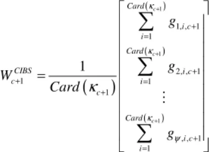
Segmentation (CIBS) from our proposal because the fundament behind the use of (n-1)D masks is to take in account geometrical and topological properties such that a 1D-KSOM use them in order to achieve and to enhance the classification. On the other hand, because of simplicity in implementing CIBS the notion of a representative, a Weights Vector, for a class is absent: the hypervoxels included in a CIBS class share the same intensity. In order to also apply our proposed FCMs to classification achieved by CIBS we build a vector representative for elements in a same class. Consider a hypervoxel v with color intensity c+1, then, it is located in class κc+1. Now, we will consider
the neighborhood of radius r for the given hypervoxel v respect to the original hypervoxelization. Then, we are
defining a (n-1)D mask whose center is v. Given value for r, the corresponding (n-1)D mask also have (2r + 1)(n-1) elements. The mask is also linearized in such way we obtain
the vector representation 1, , 1 2, , 1 , , 1 T
i c i c i c
g + g + gψ +
.
Index i only refers to an arbitrary position assigned to the mask belonging class κc+1. One of the elements in the vector
is precisely color intensity c+1 of central hypervoxel v while the rest are the color intensities of the hypervoxels inside its neighborhood. Given the above elements we build a vector representative of class κc+1, but under CIBS, as follows:
(
)
( )
( )
( )
1
1
1
1, , 1 1
2, , 1
1 1
1
, , 1 1
1
c
c
c Card
i c i
Card
CIBS i c
c i
c
Card
i c i
g
g W
Card
g
κ
κ
κ ψ
κ
+
+
+
+ =
+
+ =
+
+ =
=
∑
∑
∑
That is, given the members of class κc+1, under CIBS, its
representative has as components the average color intensity for each one of the (2r + 1)(n-1) positions in each one of the (n-1)D masks defined for the class' members. We have now representatives in order to apply them over our FCMs.
One of the aims behind the use of 1D-KSOMs for classification of points is the proper distribution of the Weights Vectors along the subspace defined by the hypercube [0, 1]ψ. We expect the Minimal Bounding Box for Weights Vectors (MBBWV) extends as much as possible over such hypercube. However, we are dealing, in our experiments, with ψ = 343 dimensions so the proposed FCMs provide us a way for analyzing, in a 2D context, how good are distributed the Weights Vectors along hypercube [0, 1]ψ. If it is false our asseveration related to the fact geometry and topology described by a neighborhood enhances classification, in particular with our 1D-KSOMs, then intensities for FCMs associated to CIBS would tend towards whiter colors than those intensities in FCMs related to 1D-KSOMs classifications. In other words, CIBS's Weights Vectors distributions should be as good, or even better, than those Weights Vectors distribution reported by the use of our proposed 1D-KSOMs.
The Table VII shows FCMs for Weights Vectors distributions associated to 1D-KSOMs described in Section IV. In these cases the maps show distribution for 80 Weights Vectors. The Table also shows FCMs for Weights Vectors, as specified in the above paragraphs, associated to CIBS. In this situation we deal with 256 Weights Vectors because, as abovementioned, CIBS takes in account all the available intensities in the grayscale. The main diagonal for the hypercube [0, 1]343, the one defined for the classification space in our experiments, has a length dmax= 343≈18.52.
Let us comment in first place observations regarding dataset VL-Sheep. The maximum distance between any two Weights Vectors under 1D-KSOM segmentation is 13.2839 while under CIBS we have a maximum distance with value 7.9367. On the other hand, minimal distances reported for 1D-KSOM segmentation and CIBS are 1.1346 and 0.0039, respectively. These values lead us to infer CIBS' MBBWV can be easily embedded in 1D-KSOM segmentation's MBBWV. Moreover, because dmax ≈ 18.52, we determine
extended over hypercube [0, 1]343 than Weights Vectors for CIBS. The average distance under 1D-KSOM segmentation is 7.7369 while it is 2.8018 under CIBS. This implies Weights Vectors for CIBS are nested in such way we cannot expect a clear differentiation of the regions occupied by the 256 classes. A simple inspection over the corresponding FCMs visually corroborates our claims by observing how intensities for FCM associated to 1D-KSOM tend towards whiter colors than those intensities in FCM related to CIBS.
In the case related to dataset Foot we found maximum distances with values 11.0783 and 3.3166 for 1D-KSOM segmentation and CIBS, respectively. Minimal distance for 1D-KSOM segmentation has value 0.1139 while for CIBS is 0.0039. Finally, 1D-KSOM segmentation's average distance is 8.1409 while it is 1.0644 under CIBS. A set of similar conclusions, just as the ones in the above paragraph, can be obtained from this case leading to effectively conclude Weights Vectors for 1D-KSOM segmentation are much better distributed in [0, 1]343 than Weights Vectors for CIBS. Our analysis based on the use of FCMs has provided us elements for concluding, in terms of the presented experiments, the validity of our asseveration related to the fact geometry and topology described by a neighborhood enhances classification of elements in a dataset.
VII.CONCLUSIONS
In this work we have listed the elements that conform to our Framework nD-EVM/Kohonen for representing in a very concise way higher dimensional hypervoxelizations. The application of 1D-KSOMs shares us an intelligent classification of the elements in a dataset in such way it is obtained a segmentation which in turn is expressed with one additional dimension under the nD-EVM. This additional dimension together with the concepts accompanying the EVM provide a representation in such way elements belonging to the same class are stored in the same geometrical entity: a couplet. Because of the way the EVM represents an orthogonal polytope it is obtained an advantage respect to spatial complexity. Our pair of experiments serves as evidence of this aspect by showing ratios Number-of-Voxels/Number-of-Extreme-Vertices 6.51 and 6.81. Moreover, we have low time complexity required for training 1D-KSOMs and the generation of the final nD-EVM representation, because these processes are achieved by means of very efficient methods and structures, such as Trie Trees in the EVM case. Thus, the dominating time is imposed precisely by the sizes of the original hypervoxelizations.
TABLE VII
FALSE COLOR MAPS ASSOCIATED TO SEGMENTATIONS FOR DATASETS VL-SHEEP AND FOOT(SEE TEXT FOR DETAILS).
FCM - 1D-KSOM for Dataset VL-Sheep (80 classes) FCM - 1D-KSOM for Dataset Foot (80 classes)
FCM - CIBS for Dataset VL-Sheep (256 classes) FCM - CIBS for Dataset Foot (256 classes)
In all maps: Maximum Distance
max 18.52
d = ψ ≈
The Framework nD-EVM/Kohonen is also the object of study and analysis in [22]. In that work there are presented five study cases where voxelizations were manipulated by 1D-KSOMs with 40 output neurons and whose training sets were specified in terms of mask radius r = 2. In [22] we report ratios Number-of-Voxels/Number-of-Extreme-Vertices were located in the range from 5.64 to 32.43, showing once again the power of conciseness our proposal has. Moreover, in [22] there are presented some error functions whose objective is to measure the quality of the representatives obtained once the corresponding 1D-KSOMs have been trained. The results are encouraging in the sense the 1D-KSOMs' Weights Vectors are better positioned than those representatives built in terms of CIBS. For more details refer to [22].
It is possible to compute other geometrical and topological interrogations over an EVM. By this way it can be obtained more information and properties about the represented datasets. There are well specified procedures under the nD-EVM which allow performing Regularized
Boolean Operations, Polytopes Splitting, Discrete
Compactness Computation, Morphological Operations, Connected Components Labeling, Boundary Extraction, among others. In [1], [14], [17], [18], [19] & [24] there are described with enough detail algorithms based in the nD-EVM which are useful and efficient for performing these interrogations and/or manipulations.
Our immediate line of future research considers certain elements presented originally in [21]. The idea is to apply
Framework nD-EVM/Kohonen in the representation and manipulation of Computer Tomography scans. We also aim to incorporate other metrics, besides the Euclidean Distance, for identifying the Winner Neuron in 1D-KSOMs' training in order to observe how it is impacted Framework
nD-EVM/Kohonen's conciseness and classification.
REFERENCES
[1] A. Aguilera, Orthogonal Polyhedra: Study and Application, PhD Thesis, Universitat Politècnica de Catalunya, 1998.
[2] M. Awad, "An Unsupervised Artificial Neural Network Method for Satellite Image Segmentation", The International Arab Journal of
Information Technology, Vol. 7, No. 2, April 2010.
[3] F. Bodon. "Surprising results of trie-based FIM algorithms", IEEE ICDM Workshop on Frequent Itemset Mining Implementations
(FIMI'04), CEUR Workshop Proceedings, Vol. 90, Brighton, United
Kingdom, November 2004.
[4] H.S.M. Coxeter, Regular Polytopes, Dover Publications, Inc., 1963. [5] E. Davalo, P. Naïm, Neural Networks, Macmillan Press Ltd, 1992. [6] Department of Radiology, University of Iowa. Web Site (February
2015): http://www.medicine.uiowa.edu/radiology/
[7] E. Friedkin, "Trie Memory", Communications of the ACM, Vol. 3, Number 9, pp. 490-499, 1960.
[8] J. Hilera, V. Martínez, Redes Neuronales Artificiales (Artificial Neural Networks), written in Spanish, Alfaomega, 2000, México. [9] J. Jiang, P. Trundle, J. Ren, "Medical image analysis with artificial
neural networks", Computerized Medical Imaging and Graphics, 34, pp. 617–631, 2010, Elsevier.
[10] A. Jonas, N. Kiryati, “Digital Representation Schemes for 3-D Curves”, Technical Report CC PUB #114, The Technion - Israel Institute of Technology, Haifa, Israel, 1995.
[11] G. Klajnsek, B. Rupnik, D. Spelic, “An Improved Quadtree-based Algorithm for Lossless Compression of Volumetric Datasets”, 6th WSEAS Int. Conference on Computational Intelligence, Man-Machine
Systems and Cybernetics, 1:264-270, Spain, December 2007.
[12] S. Marchand-Maillet, Y.M. Sharaiha, Binary Digital Image
Processing: A Discrete Approach, Academic Press, 1999.
[13] R. Pérez Aguila, P. Gómez-Gil, A. Aguilera, "Non-Supervised Classification of 2D Color Images Using Kohonen Networks and a Novel Metric", Lecture Notes in Computer Science, Vol. 3773, pp. 271-284. Springer-Verlag Berlin Heidelberg, 2005.
[14] R. Pérez-Aguila, Orthogonal Polytopes: Study and Application, PhD Thesis, Universidad de las Américas - Puebla (UDLAP), 2006. http://catarina.udlap.mx/u_dl_a/tales/documentos/dsc/perez_a_r/ [15] R. Pérez-Aguila, “Modeling and Manipulating 3D Datasets through
the Extreme Vertices Model in the n-Dimensional Space (nD-EVM)”, Research in Computer Science, Special Issue:
Industrial Informatics, México, 31:15-24, 2007.
[16] R. Pérez-Aguila, "Brain Tissue Characterization Via Non-Supervised One-Dimensional Kohonen Networks", Proc. of the XIX International Conference on Electronics, Communications and Computers
CONIELECOMP 2009, pp. 197-201. IEEE Computer Society.
February 26-28, 2009. Cholula, Puebla, México.
[17] R. Pérez-Aguila, “Computing the Discrete Compactness of Orthogonal Pseudo-Polytopes via Their nD-EVM Representation”,
Mathematical Problems in Engineering, vol. 2010, Article ID
598910, 28 pages, 2010. doi:10.1155/2010/598910
[18] R. Pérez-Aguila, "Towards a New Approach for Modeling Volume Datasets Based on Orthogonal Polytopes in Four-Dimensional Color Space", Engineering Letters, Vol. 18, Issue 4, pp. 326-340, ISSN: 1816-0948 (online), 1816-093X (print), IAENG, November 2010. [19] R. Pérez-Aguila, "Efficient Boundary Extraction from Orthogonal
Pseudo-Polytopes: An Approach Based on the nD-EVM", Journal of
Applied Mathematics, vol. 2011, Article ID 937263, 29 pages, 2011,
doi: 10.1155/2011/937263. ISSN: 1110-757X, e-ISSN: 1687-0042. [20] R. Pérez-Aguila, Una Introducción al Cómputo Neuronal Artificial
(An Introduction to Artificial Neural Computing), written in Spanish, El Cid Editor, Argentina, First Edition, September 2012, ISBN (Print): 978-1-4135-2424-6, ISBN (Digital): 978-1-4135-2434-5. [21] R. Pérez-Aguila, "Enhancing Brain Tissue Segmentation and Image
Classification via 1D Kohonen Networks and Discrete Compactness: An Experimental Study", Engineering Letters, Vol. 21, Issue 4, pp. 171-180, ISSN: 1816-0948 (online), 1816-093X (print), IAENG, Nov. 2013.
[22] R. Pérez-Aguila, R. Ruiz-Rodríguez, "Concise and Accessible Representations for Multidimensional Datasets: Introducing a Framework Based on the nD-EVM and Kohonen Networks",
Applied Computational Intelligence and Soft Computing,
Vol. 2015, Hindawi Publishing Corporation, 2015. Web Site: http://www.hindawi.com/journals/acisc/2015/676780
[23] H. Ritter, T. Martinetz, K. Schulten, Neural Computation and
Self-Organizing Maps, An introduction, Addison-Wesley, 1992.
[24] J. Rodríguez, D. Ayala, “Erosion and Dilation on 2D and 3D Digital Images: A new size-independent approach”, Vision Modeling and
Visualization 2001, Germany, 1:143–150, 2001.
[25] S. Roettger, The Volume Library. Web Site (last visit in September, 2014): http://www9.informatik.uni-erlangen.de/External/vollib/ [26] R. Ruiz-Rodríguez, Implementación del EVM (Extreme Vertices
Model) en Java, M.Sc Thesis, UDLAP, 2002.
http://catarina.udlap.mx/u_dl_a/tales/documentos/msp/ruiz_r_r/ [27] R. Ruiz Rodríguez, "A 3D Editor for Orthogonal Polyhedra Based on
the Extreme Vertices Model", Décimo Congreso Internacional de
Investigación en Ciencias Computacionales CIICC 03, Oaxtepec,
Morelos, México, Octubre 2003. ISBN: 968-5823-02-2.
[28] R. Ruiz Rodríguez, "Using the Ordered Union of Disjoint Boxes Model for the Visualization as Solid Objects of Orthogonal Pseudo Polyhedra Defined in the Extreme Vertices Model", II Congreso
Internacional de Informática y Computación de la ANIEI, ANIEI
2003, Zacatecas, Zacatecas, México, Octubre 2003.
[29] D.M.Y. Sommerville, An Introduction to the Geometry of N
Dimensions, Dover Publications Inc., 1958.
[30] W. Song, S. Hua, Z. ou, H. An, K. Song, “Octree Based Representation and Volume Rendering of Three-Dimensional Medical Data Sets”, International Conference on BioMedical
Engineering and Informatics 2008, 1:316-320, 2008.
[31] M. Spivak, Calculus on Manifolds: A Modern Approach to Classical
Theorems of Advanced Calculus, HarperCollins Publishers, 1965.
[32] N. Torbati, A. Ayatollahi, A. Kermani, "An efficient neural network based method for medical image segmentation", Computers in
biology and medicine, 44:76-87, 2014.
[33] University of Tübingen. The Official Volren and Volvis Homepage. Web Site (last visit in September, 2014): http://www.gris. uni-tuebingen.de/edu/areas/scivis/volren/software/software.html [34] K. Yuan, F. Peng, S. Feng, W. Chen, "Pre-Processing of CT Brain
Images for Content-Based Image Retrieval", Proc. International
Conference on BioMedical Engineering and Informatics 2008, Vol. 2,
pp. 208-212.
[35] J. Zerubia, S. Yu, Z. Kato, M. Berthod, "Bayesian Image Classification Using Markov Random Fields", Image and Vision