Citizen Science Program Shows Urban Areas
Have Lower Occurrence of Frog Species, but
Not Accelerated Declines
Martin J. Westgate1*, Ben C. Scheele1, Karen Ikin1,2, Anke Maria Hoefer3, R. Matthew Beaty4, Murray Evans5, Will Osborne6, David Hunter7, Laura Rayner1, Don A. Driscoll2,8
1Fenner School of Environment and Society, The Australian National University, Canberra, ACT, 2601, Australia,2ARC Centre of Excellence for Environmental Decisions, The Australian National University, Canberra, ACT, 2601, Australia,3ACT and Region Frogwatch, Ginninderra Catchment Group, Canberra, ACT, 2615, Australia,4CSIRO Land and Water, Canberra, ACT, 2601, Australia,5Environment and Planning Directorate, ACT Government, Canberra, ACT, 2601, Australia,6Institute for Applied Ecology, University of Canberra, Canberra, ACT, 2601, Australia,7NSW Office of Environment and Heritage, Queanbeyan, NSW, 2620, Australia,8School of Life and Environmental Sciences, Centre for Integrative Ecology, Deakin University, Melbourne Burwood Campus, Burwood, VIC, 3125, Australia
Abstract
Understanding the influence of landscape change on animal populations is critical to inform biodiversity conservation efforts. A particularly important goal is to understand how urban density affects the persistence of animal populations through time, and how these impacts can be mediated by habitat provision; but data on this question are limited for some taxa. Here, we use data from a citizen science monitoring program to investigate the effect of urbanization on patterns of frog species richness and occurrence over 13 years. Sites sur-rounded by a high proportion of bare ground (a proxy for urbanization) had consistently lower frog occurrence, but we found no evidence that declines were restricted to urban areas. Instead, several frog species showed declines in rural wetlands with low-quality habi-tat. Our analysis shows that urban wetlands had low but stable species richness; but also that population trajectories are strongly influenced by vegetation provision in both the ripar-ian zone and the wider landscape. Future increases in the extent of urban environments in our study area are likely to negatively impact populations of several frog species. However, existing urban areas are unlikely to lose further frog species in the medium term. We recom-mend that landscape planning and management focus on the conservation and restoration of rural wetlands to arrest current declines, and the revegetation of urban wetlands to facili-tate the re-expansion of urban-sensitive species.
OPEN ACCESS
Citation:Westgate MJ, Scheele BC, Ikin K, Hoefer AM, Beaty RM, Evans M, et al. (2015) Citizen Science Program Shows Urban Areas Have Lower Occurrence of Frog Species, but Not Accelerated Declines. PLoS ONE 10(11): e0140973. doi:10.1371/ journal.pone.0140973
Editor:Benedikt R. Schmidt, Universität Zurich, SWITZERLAND
Received:January 18, 2015
Accepted:October 2, 2015
Published:November 18, 2015
Copyright:© 2015 Westgate et al. This is an open access article distributed under the terms of the
Creative Commons Attribution License, which permits unrestricted use, distribution, and reproduction in any medium, provided the original author and source are credited.
Data Availability Statement:All data necessary to duplicate our findings are available from Dryad (Title: Data from: Citizen science program shows urban areas have lower occurrence of frog species, but not accelerated declines. DOI: doi:10.5061/dryad.75s51).
Introduction
The majority of the human population now lives in urban areas [1], and the total area devoted to urban land uses continues to rise in many regions of the world [2]. Although this process is considered to be broadly detrimental to biodiversity [3,4], urban areas are capable of sustaining diverse plant and animal assemblages in many instances [5,6]. Further, biodiverse cityscapes provide a range of ancillary benefits, including greater integration with water-sensitive urban design [7], mitigation of urban heat island effects [8], and improved human well-being through greater association and engagement with nature [9]. While maintaining diverse plant commu-nities may be achieved through preservation or revegetation, conservation of urban animal populations is much more challenging. Therefore, a valuable goal for ecology is to identify cir-cumstances where landscape planning can be used to facilitate the persistence of threatened or valued animal species in urban and peri-urban areas. This goal requires identification of attri-butes of those areas (such as the quality and availability of suitable habitats) that are associated with declines or expansions of biodiversity.
While the study of urban biodiversity has expanded significantly in recent years [5], consid-erable gaps remain in our knowledge of how urbanization drives ecosystem change. As such, it is often unclear how new and existing urban environments can be planned and managed to facilitate the persistence of biodiversity. For example, studies of urban bird populations have shown that retention of keystone structures such as large old trees can have a strong, positive effect on suburban biodiversity [10], but this effect is also dependent on urban density [11]. Further, some threatened species respond negatively to the rate of expansion of urbanization, irrespective of whether their home range is directly impacted [12]. These studies highlight that urbanization has a range of correlated impacts on animal populations, meaning that it can be difficult to predict which management or planning activities will be of greatest benefit to biodi-versity. They also suggest that piecemeal changes to urban density, the rate of urban expansion, or the attributes of urban parks and gardens are unlikely to be effective at retaining biodiversity in urban locations when implemented in isolation [11].
A further reason it is difficult to quantify the effects of urban planning on biodiversity is that these effects can manifest over several years or even decades, a time-scale for which com-prehensive survey data are rarely available [13,14]. Consequently, studies of the effects of urbanization typically involve short-term studies of differences in biotic assemblages across an urbanization gradient [15], or between towns or cities of differing age [16]. While these approaches provide valuable results in many cases, space-for-time substitution can confound site and treatment effects, and does not allow the trends of individual populations to be observed through time [17,18]. An effective alternative is to use long-term datasets collected through citizen science initiatives, which often provide much higher spatial and temporal repli-cation than expert surveys at lower cost [19,20]. These datasets have potentially enormous util-ity for investigating questions about the patterns and drivers of biotic change [21], provided that potential sampling biases are addressed in a rigorous statistical framework [22]. Citizen monitoring of plant or animal populations is particularly valuable in urban areas where volun-teers (and therefore records) are proportionally more common [23,24].
In this paper, we use a 13-year citizen science dataset to investigate how urbanization influ-ences the occurrence or trajectory of frog populations, and the extent to which these effects are altered by vegetation structure at (or around) wetland habitats. Quantifying trends in urban frog populations is important because changes in the type and intensity of human land use rep-resent one of the most significant threats to amphibian biodiversity [25]. Further, while the effect of urbanization on frog populations is generally thought to be negative [26], some urban areas sustain high densities of frog populations [27,28], in some cases even preserving relictual
research. The funders had no role in study design, data collection and analysis, decision to publish, or preparation of the manuscript.
populations of species that have been devastated by disease [29]. Finally, although factors such as vegetation cover have been shown to influence frogoccurrencein urban ecosystems [30–33], there has been less work to understand how these variables interact to influence population tra-jectories(although see ref [34]). Here, we seek to address these knowledge gaps via a case study from a temperate, modern city in southeastern Australia (Canberra).
We made severala prioripredictions as to the kinds of patterns that we expected to observe during our analysis, based on prior research in our study region and elsewhere. In particular, we did not anticipate a decreasing trend in species richness over our study period, as unlike many other locations [35,36], the disease chytridiomycosis no longer appears to be causing declines in our study region, despite previous extinctions and ongoing high prevalence [37]. However, important population-level processes such as breeding and dispersal are impeded by the loss of wetlands and terrestrial habitat that occurs during urbanization [30]. Our metric of urban land cover–the percentage cover of bare ground within the landscape surrounding each survey location–is a proxy for several such processes. Therefore, we expected to observe faster declines of some frog species in areas of high urbanization; i.e. that there would be an interac-tion between urban land cover and survey year as predictors of frog occurrence. We also antici-pated that several hydrological wetland attributes–including their size, water flow rate, and spatial arrangement–would influence their probability of occupation by frog species, and so controlled for these effects by including them as covariates in our analyses.
Materials and Methods
Ethics statement
This field study was established under the direction of the Australian Capital Territory (ACT) Government Environment and Sustainable Development Directorate and the University of Canberra. Sampling was strictly observation-only and no animal handling was involved. The study was conducted on public and privately-owned land, and access permission was granted by landowners prior to establishing the field sites.
Study area and species
Our study was undertaken in the Canberra region of the Australian Capital Territory (ACT) and included surrounding areas of New South Wales (NSW), southeastern Australia (Fig 1). This relatively small geographic area (~2,500 square kilometres, 37.3’S, 149.1’E) contains a population of ~380,000 people, and has low precipitation relative to adjacent coastal and mountain regions (mean annual precipitation = ~690mm). Importantly, our study began dur-ing the severe Australian Millennium drought, which ended in 2009 [38]. Consequently, our results must be interpreted considering the potential for climate-based fluctuations in water availability–and therefore in frog populations–over our study period.
initiatives that regularly monitor bird and frog populations throughout the Canberra region (e.g. see [41]), providing a valuable source of information on population trajectories.
Eighteen species of frogs are known from the ACT and nearby regions [42]; however only ten species currently occur in or near urban areas. We had sufficient data to investigate the occurrence of eight species from three families (Hylidae:Litoria peroniiandLitoria verreauxii; Limnodynastidae:Limnodynastes dumerilii,Limnodynastes peroniiandLimnodynastes tasma-niensis; Myobatrachidae:Crinia signifiera,Crinia parinsigniferaandUperoleia laevigata). The remaining two species (Litoria auraandNeobatrachus sudelli) were exceptionally rare in our Fig 1. Map of Frogwatch survey locations.Sealed roads are solid blue lines.
dataset, and so we restricted our investigation of species richness to the same eight species dis-cussed above.
The Frogwatch dataset
We built our models of frog species occurrence and richness using data generated by the Frog-watch ACT and Region Program (hereafter referred to as‘Frogwatch’), a citizen science initia-tive that has been run by the Ginninderra Catchment Group since 2002. Sites were selected by volunteers, and consisted of a single surveyable portion of the wetland edge. This definition ensures compatibility between vegetation and frog attributes, but also means that our data rep-resents a subset of the total habitat available in large lakes or rivers. Fieldwork in the Frogwatch program uses auditory sampling to record occurrence of calling males, following a standard-ized procedure. Surveys may be taken at any time during October each year (during the austral spring when most species are breeding), although the majority of surveys occur during the des-ignated‘census week’(beginning from the third Sunday in October). All volunteers make an initial site visit during the day to record attributes of the pond or waterway that they are inves-tigating. This is followed by an evening visit (between sunset and 10pm) to identify calling frog species, along with associated weather and water and air temperature. Surveys include taking audio recordings of the frog chorus which are validated by the Frogwatch coordinator (AMH) prior to inclusion in the dataset.
For the purpose of this analysis, we used data collected between 2002 and 2014 (inclusive), incorporating 3,967 visits to 486 unique sites (Fig 1). However, we removed 148 sites as they were visited on<3 occasions during the study period, which can increase the difficulty of
fit-ting mixed models in analyses such as ours [43]. We excluded a further 18 sites because they lacked data on one or more site-level covariates. This left us with data from 3,633 visits to 320 sites for further analysis. Sites were visited an average of 11.3 times over the 13 years
(median = 8 visits), in an average of 5.2 of the 13 survey years, while 28 sites (9%) were visited in ten or more years.
Site-level predictor variables
We investigated the effects of seven site-level predictor variables, derived from three distinct sources. The first was a set of general hydrological or vegetation attributes for each site, which we quantified using volunteer responses to site survey questionnaires. The first of these was a binary variable (waterbody type) that described whether a site contained still or flowing water. We chose the most common response amongst all visitors to each site as the‘correct’value for this variable. The second was a continuous variable describing the estimated size of each water-body, calculated as the mean of all reported, log10-transformed waterbody areas (in metres
squared) for each site. Finally, we used volunteer descriptions of terrestrial and aquatic vegeta-tion to estimate the quality of local vegetavegeta-tion at each site. Aquatic vegetavegeta-tion was scored as zero if50% of visitors to that site reported no vegetation, one if only algae was reported, two if aquatic or emergent vegetation was present, and three if both aquatic and emergent vegeta-tion were reported. Terrestrial vegetavegeta-tion was recorded as the number of reported vegetavegeta-tion strata (under-, mid- and over-storey) at each site. Our final variable (local vegetation) summed these two metrics to give a continuous, numerical variable describing vegetation extent. For all of the volunteer-derived covariates, high variability in volunteer responses forced us to assume no change in these variables over time at each site.
variables (described below) from all pixels within a buffer of 500 metre radius, excluding any pixels that were recorded as water. The first variable, representing urbanization, gave the pro-portional area of bare ground, which we use as a proxy of percent urban land cover. Bare ground was a useful proxy for urbanization because it was strongly correlated with a more direct measure of urban density (i.e. road length within a 500 metre buffer) in our study region, and was available for all study years. Although this variable was continuously distributed (rang-ing from 1% to 35% bare ground cover), we refer to sites with extreme values of this variable as either‘rural’(tenth percentile) or‘urban’(ninetieth percentile). We categorized sites in this way for clarity; but as Canberra is a low density city by global standards [1], readers should not consider‘urban’sites in our analysis as comparable to high density urban locations in other cit-ies. The second variable gave the percent cover of canopy vegetation. As both variables were skewed towards very low values, we logit-transformed both covariates prior to including them in our analysis. Unlike our volunteer-derived variables, we used annual data for MODIS-derived variables, and so our analysis investigates the effect of urbanization and canopy cover while allowing both values to change at each site over the study period.
The third set of variables was included to account for potential statistical anomalies in our dataset. We derived a factorial variable describing the identity of each site for use as a random effect. We also calculated a spatial autocovariate for each response variable using the autocov_-dist function from the spdep R package [45], to account for spatial structuring of species rich-ness or occurrence patterns. In datasets where survey effort is inconsistent, a variable
describing the number of species observed per visit (the‘list length’) is often informative [46]; however this was not necessary in our case as survey effort per visit is standardised in the Frog-watch program.
Prior to our analysis, we scaled all continuous predictor variables (i.e. local vegetation, % urban, % canopy and all spatial autocovariates) to a mean of zero and a standard deviation of one. As a result, all coefficients presented can be compared between each other, or between models for different species.
Statistical analysis
We used generalized linear mixed models (GLMMs) to model variation in species richness and occurrence, including a list of site identifiers as a random effect to account for non-indepen-dence caused by repeat visits to each site [43]. We were unable to fit models that account for variable detection rates (e.g. [47]) because sites were not visited consistently each year, and because some species were too rare to parameterize such a model. Consequently, our approach confounds occupancy and detection, meaning that we are unable to identify what proportion of change in observation rates resulted from change in species distributions, rather than changes in detectability. Further, interpreting our results purely in terms of occupancy rates requires the assumption that detection does not vary systematically in relation to our predictor variables, which may be unrealistic. However, simulations have shown [48] that the data collec-tion, cleaning and analysis methods that we used–including consistent effort per visit, removal of rarely visited sites from the dataset, and accounting for site-specific observation probabili-ties–results in a model that has low risk of systematic bias, and only marginally increased type I error (i.e. mistakenly identifying strong effects that are not present) without an increase in type II error (likelihood of missing strong effects when they are present). We therefore report our results without further reference to detection probabilities, while acknowledging that such research would be informative.
species richness model will be strongly related to the sum of the eight individual species models that we also present; however we include it in our analysis for completeness, and because rich-ness is a common summary statistic of use in the management of frog populations in our study region. We used these models to test a range of hypotheses regarding the influence of urbaniza-tion and vegetaurbaniza-tion on occurrence or trajectory of frog populaurbaniza-tions using a model selecurbaniza-tion approach (Table 1). We calculated all models using the lme4 package [49] in the R statistical program [50], and selected the‘best’model as that with the lowest AICc[51], while treating all
models within two AICcof the best model as plausible.
Results
Model selection by AICcshowed that complex models were nearly always selected to describe
frog population trajectories in our study region, with models that included interactions being strongly weighted for six of eight species, as well as for species richness (Table 2). This consti-tutes strong support for the hypothesis that frog population trajectories vary between sites with differing urban land cover and vegetation attributes. However, we were unable to conclusively determine a final model for half of our eight species. Model selection was particularly equivocal for two species from the genusLimnodynastes; namelyLim.dumerilii(four models withΔAICc
<2) andLim.peronii(five models withΔAICc<2). We were also unable to discriminate
between very similar models forC.signiferaandLim.tasmaniensis(Table 2).
We found strong, negative effects of urban land cover on the occurrence of six of the eight species that we studied (i.e. all species exceptLim.peroniiandLit.verreauxii), as well as lower species richness in urban than rural wetlands (Fig 2). Further, large wetlands were more likely to contain individuals from all species exceptLim.peronii, while half of the eight species we studied were more likely to be found in still than flowing water (in contrast,Lim.dumeriliiwas
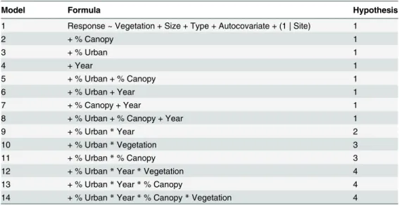
Table 1. Outline of all models tested for relative fit to frog occurrence or richness patterns.
Model Formula Hypothesis
1 Response ~ Vegetation + Size + Type + Autocovariate + (1 | Site) 1
2 + % Canopy 1
3 + % Urban 1
4 + Year 1
5 + % Urban + % Canopy 1
6 + % Urban + Year 1
7 + % Canopy + Year 1
8 + % Urban + % Canopy + Year 1
9 + % Urban*Year 2
10 + % Urban*Vegetation 3
11 + % Urban*% Canopy 3
12 + % Urban*Year*Vegetation 4
13 + % Urban*Year*% Canopy 4
14 + % Urban*Year*% Canopy*Vegetation 4
All models include all terms in model 1, plus those terms listed in the‘formula’column for that model. Hypotheses: 1. Occurrence or richness of frog species is affected by waterbody attributes, and/or is changing over time; 2. The effect of time on frog occurrence or richness varies across the urbanization gradient; 3. The effect of time on frog occurrence or richness varies across the urbanization gradient; 4. The effect of time on frog occurrence or richness is influenced by urbanization and one or more vegetation-related attributes.
less likely to occur in still water). Finally, site-level vegetation was positively related to the likeli-hood of observing the majority of frog species, while percentage canopy cover within 500m had either no effect or a moderate negative association with frog occurrence.
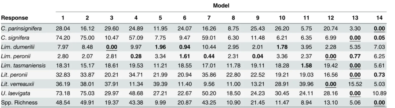
Although most frog species were less likely to be found in urban than rural wetlands, our model selection results (Table 2) suggested that the effect of urbanization on population trajec-tories was complex, and interacted with site-level and landscape-wide vegetation patterns. Plot-ting results from all‘best’models that included an effect of time (i.e. for all species exceptLim. Table 2. Change in AICcfrom the‘best’model of frog species occurrence or richness.
Model
Response 1 2 3 4 5 6 7 8 9 10 11 12 13 14
C.parinsignifera 28.04 16.12 29.60 24.89 11.95 24.07 16.26 8.75 25.43 26.20 5.75 20.74 3.30 0.00
C.signifera 74.20 75.00 10.47 57.09 7.75 9.47 59.01 6.30 11.48 6.21 6.35 6.99 0.00 0.05
Lim.dumerilii 7.97 8.48 0.00 9.97 1.96 0.94 10.44 2.95 2.01 1.78 3.95 2.28 5.35 7.03
Lim.peronii 2.80 2.07 2.81 0.28 3.34 1.61 0.44 2.31 0.04 3.36 2.37 0.00 0.77 6.25
Lim.tasmaniensis 18.31 15.17 18.61 19.53 11.21 18.55 17.01 11.78 19.11 18.28 1.58 19.42 0.00 5.61
Lit.peronii 32.83 33.87 20.21 34.71 21.99 20.94 35.86 22.80 22.52 19.21 19.03 16.56 0.00 0.73
Lit.verreauxii 36.19 38.01 37.91 11.34 39.39 11.40 9.56 11.00 13.21 28.91 39.96 0.00 15.52 5.03
U.laevigata 73.18 75.03 29.97 48.68 27.21 22.67 50.20 18.50 24.23 30.45 24.11 28.16 0.00 10.89
Spp. Richness 48.54 49.91 19.37 43.38 9.99 20.87 43.25 10.90 21.45 11.47 8.94 13.10 5.06 0.00
All models with AICc<2 shown in bold, with‘top’model for each species underlined. Note that model formulae are given inTable 1.
doi:10.1371/journal.pone.0140973.t002
Fig 2. Coefficient estimates from final models for each species.Plots are ordered by mean effect size (calculated as the coefficient divided by the standard error of that coefficient) across all models, with highest effect size on the left and lowest on the right. Species are shown in increasing order of prevalence (top to bottom). Colours are to distinguish between plots only, and do not have any inherent meaning. Only variables included in the final model are shown (hence missing values in panel f), while interactions are not shown. Axes vary in scale between subplots.
dumerilii) supported this expectation, showing that none of the species that we studied have declined consistently within urban areas (Fig 3). Instead, the fastest declines in our study region appear to be occurring in rural areas. For example,Lit.peronii(Fig 3F) andU.laevigata(Fig 3G) are both declining in rural areas with low canopy cover, but increasing in prevalence in rural areas with high canopy cover. Similarly,Lim.peronii(Fig 3A) appears to be declining only in rural wetlands with high site-level vegetation; but this is the result of a model with low weight and should not be considered conclusive. In contrast, every species showed increases in prevalence in at least a subset of urban areas, although these increases were generally small and from a low baseline. Overall, therefore, our results show that frog trajectories in urban areas are highly conditional on the amount of vegetation at the pond and in the surrounding landscape.
Discussion
In this study, we investigated trends in the composition and richness of frog assemblages from an urban landscape in southeastern Australia, using a citizen science dataset of high spatial and temporal resolution. Consequently, our results provide a comprehensive insight to the viability Fig 3. Modelled frog occurrence and species richness over time in the ACT region.
of frog populations in our study region, showing that several species occur at lower incidence in urban areas. However, urban populations were relatively stable over the 13 years of observa-tion, suggesting that many frog species may be able to persist in these locations in the medium-to long- term (albeit at a low proportion of available wetlands; seeFig 3). Even more encourag-ingly, the majority of species in our study were increasing in prevalence in well-vegetated urban wetlands. This suggests that local conservation and remediation activities might be capa-ble of sustaining both urban and rural frog populations. We further discuss these results and their implications in the remainder of our paper.
Influence of urban density on frog assemblages
Our results clearly show that urban areas within the Canberra region support lower richness and incidence of frog species than their rural equivalents. In particular, six of the eight species that we studied (i.e. all exceptLim.peroniiandLit.verreauxii) showed strong, negative effects of urban density on their probability of occurrence (Fig 2). While the precise mechanism by which urbanization influences frog populations remains unclear, it is likely that urbanization influences frog dispersal rates, as well as the quality of aquatic habitats for frog survival and reproduction [52]. For example, urban environments strongly reduce the rate of frogs’ inter-pond movements [53], and may increase the probability that frogs will suffer predation from pets [54], reducing the chance that local populations can be maintained via colonization (and thereby reducing the overall occupancy rate; see [55]). This supports earlier research showing that urban wetlands display a series of correlated attributes that reduce habitat suitability for many frog species [30].
Despite lower richness and incidence of frog species in urbanized areas, our results indicate that urban sites can sustain some frog species through time [52]. In particular, we found no evi-dence of ongoing declines in urban areas for any species (Fig 3). This finding supports research from other locations showing persistence of frog populations in cities that are older than Can-berra by several decades [30] or even centuries [56], and suggests that urbanization may not induce the long extinction lags that have been recorded in other taxonomic groups such as plants [16] or butterflies [15]. However, the lower incidence and diversity of frog species in urban areas indicates that urban-sensitive species may have already gone extinct in highly urbanised sites. Our results therefore suggest that increasing urbanization over time–either by expansion of the urban boundary, or increasing density of existing suburbs–is likely to be asso-ciated with further declines in frog populations in our study region.
Contrary to our predictions, we found that several frog species (Lit.peronii,U.laevigataand possiblyLim.peronii) appear to have declined rapidly in some rural wetlands around Canberra (Fig 3D and 3E). Why declines should be largely restricted to rural areas during our study period, and to these species in particular, is unclear. One possibility is that–as our data are collected in the same month each year–changes in breeding phenology could appear as declines in our analy-sis, suggesting a potential influence of climate change on our results [57]. Alternatively, undocu-mented changes to rural ponds may have occurred near Canberra during our study period. For example, changes to agricultural practices such as fertilizer use or stocking rates could potentially have influenced occupancy rates of these two species (see [58]). Finally–and in common with all forms of statistical investigation–our results are subject to error, and so some caution is required in interpreting the precise rate and location of population declines that we report. Nonetheless, identifying the relative importance of these processes for driving changes in frog assemblages should be a priority for future research, to allow targeted activities to prevent any such declines.
our results suggest that increases in landscape-wide canopy cover (forLim.tasmaniensis,C. sig-nifera and Lit.peronii), site-level vegetation cover (forLim.peronii), or both (forC. parinsigni-fera), can reduce or even reverse population declines. However, two important caveats to these conclusions should be made. First, our results are correlative and should not be confused with experimental results; it is possible that some unmeasured attribute of urban wetlands is respon-sible for the changes in frog populations that we have documented (although see [59]). Second, the effects of each vegetation variable varied enormously between species, between locations, and in relation to their respective effects on occupancy rates or population trajectories. For example, high canopy cover was associated with increases in prevalence ofU.laevigatain rural areas, but led to decreased prevalence in urban areas (Fig 3G). Similarly, sites with low canopy cover and low site-level vegetation had the highest occupancy rates ofC.parinsigniferain rural areas, but the lowest occupancy rates in urban areas (Fig 3D). Therefore, planners seeking to facilitate the survival of frog populations in our study region should consider the habitat requirements of those species they most wish to benefit, as any single intervention will benefit some species more than others.
Overall, our results suggest that large, still, well-vegetated wetlands in rural areas are most likely to sustain diverse frog assemblages in our study region. In particular, high levels of aquatic vegetation always had a positive effect on species occurrence, and for five of our study species (C.signifera,Lit.verreauxii, and all threeLimnodynastesspp.) this effect was stronger than the negative effect of urbanization. This is encouraging, as it suggests that prevalence of frogs in urban areas may be increased by revegetation of frog breeding sites. Our work also con-tradicts evidence [60] that permanent flooding is largely detrimental to frog populations (Fig 2), possibly because most large, still wetlands in our study region are artificial and so lack diverse assemblages of predatory fish. In combination, these results suggest that comparably straightforward management interventions (such as stock exclusion in rural areas, and revege-tation in urban wetlands) could provide large benefits to frog populations across our study region [61].
Future directions
Citizen science initiatives are becoming increasingly common in a number of disciplines, and our results highlight both the strengths and potential pitfalls of such datasets (see also [20]). In particular, citizen science programs typically provide good data on common species [62], which are valuable for assessing long-term changes in biodiversity resulting from climate change or land use shifts. Long-term datasets–and long-term public engagement with nature– also help to counteract the‘shifting baselines’problem, whereby management goals become less stringent with time due to altered perception of the‘ideal’ecosystem state [63]. In contrast, a widely recognized limitation of citizen science is that there is limited scope to customize mon-itoring to focus on particular locations, species, or trends [64]. For example, species of conser-vation concern often require specialised, intensive monitoring programs [65], and so their population status can be difficult to assess using citizen-based approaches. Similarly, attributes of ecosystems that are undetectable through passive observation require specialist assessment, of which an important example in our study is the distribution and impact of chytrid fungus [37]. Consequently, it is important when assessing the value of citizen science initiatives to con-sider both the strengths and weaknesses of this method of monitoring biodiversity.
of these declines. This is indicative of a broader issue with studies such as ours, namely that sta-tistical power to detect long-term, shallow declines in animal populations is typically low [66], and can only be achieved through monitoring over longer periods than Frogwatch has achieved to date [67]. Further, our process of removing rarely visited sites from the dataset prior to anal-ysis is known to reduce statistical power for detecting trends (i.e. to increase type II error [48]). Finally, the structure of our data necessitated that we confound occupancy and detection in our analysis, with the result that we are unable to report estimates of absolute occupancy rates. These considerations are important from a management perspective because they reduce our capacity to identify and intervene in population declines. Fortunately, the problems that we have outlined above could be substantially addressed by focussing available research effort on a smaller number of sites, while ensuring that each site was consistently visited on more than one occasion per year. Although direction of research effort is difficult in any volunteer pro-gram [64], this strategy has now been adopted as a guiding principle for future work in the ACT Frogwatch program.
In addition to statistical issues, the distribution of research effort in the Frogwatch program also biased our conclusions towards species that were tolerant of urban environments. This meant that we were unable to reach any conclusions regarding the trajectory of several species in our study region, including any species that were restricted to riverine or montane environ-ments. For example, we were able to verify the documented expansion ofLit.verreauxiiin our study region over recent years (seeFig 3E, [37]), but were unable to test anecdotal suggestions thatLitoria latopalmatamay also be expanding (W. Osborne, pers. obs.). Similarly, Neobatra-chus sudellidisplays explosive breeding following high rainfall events, and so is rarely detected by Frogwatch volunteers, reducing our knowledge of the distribution and trajectory of this spe-cies. Despite these knowledge gaps, we do not advocate the expansion of the existing program to accommodate a wider range of survey sites and seasons, as this strategy would be inconsis-tent with our call for more targeted data collection at a smaller number of sites (see above). Instead, we suggest that if there is a strong need for data on cryptic or rarely detected species, then that data should be collected by professional ecologists as part of a targeted monitoring program [58,64].
Conclusions
Using a long-term citizen science dataset, we have quantified the association between wetland attributes and the distribution and trajectory of frog populations in an urban landscape. Our results show that the effects of urbanization are mediated by wetland vegetation structure and canopy cover in the surrounding landscape. Frog declines in the Canberra region are largest in the rural hinterland, with urban frog populations persisting at a comparatively small propor-tion of available wetlands (see also [68]). However, there was little evidence of widespread declines in urban wetlands, with populations of some species marginally increasing in preva-lence in urban areas with suitable site-level or landscape-wide vegetation. These findings pro-vide robust support for landscape planning and management to sustain diverse frog
assemblages in our study region. We suggest that the greatest opportunity for frog conservation in our study region is through the conservation and restoration of rural wetlands to arrest cur-rent declines. In comparison, revegetation of urban wetlands has strong potential as a method to facilitate the re-expansion of urban-sensitive species.
Acknowledgments
Rochelle McConville, Beth Mantle and Emma Keightley for their past work in the establish-ment and continuation of this program.
Author Contributions
Conceived and designed the experiments: AMH ME WO. Analyzed the data: MJW RMB KI LR. Wrote the paper: MJW BCS KI AMH RMB ME WO DH LR DAD.
References
1. United Nations Department of Economic and Social Affairs: Population Division (2014) World urbaniza-tion prospects: The 2014 revision.
2. Seto KC, Fragkias M, Güneralp B, Reilly MK (2011) A meta-analysis of global urban land expansion. PLoS ONE 6: e23777. doi:10.1371/journal.pone.0023777PMID:21876770
3. Pautasso M (2007) Scale dependence of the correlation between human population presence and ver-tebrate and plant species richness. Ecol Lett 10: 16–24. PMID:17204113
4. Radeloff VC, Stewart SI, Hawbaker TJ, Gimmi U, Pidgeon AM, Flather CH, et al. (2010) Housing growth in and near United States protected areas limits their conservation value. Proc Natl Acad Sci U S A 107: 940–945. doi:10.1073/pnas.0911131107PMID:20080780
5. Aronson MFJ, La Sorte FA, Nilon CH, Katti M, Goddard MA, Lepczyk CA, et al. (2014) A global analysis of the impacts of urbanization on bird and plant diversity reveals key anthropogenic drivers. P Roy Soc B—Biol Sci 281.
6. Schwartz MW, Jurjavcic NL, O'Brien JM (2002) Conservation's disenfranchised urban poor. Bioscience 52: 601–606.
7. Kazemi F, Beecham S, Gibbs J (2011) Streetscape biodiversity and the role of bioretention swales in an Australian urban environment. Landsc Urban Plan 101: 139–148.
8. Feyisa GL, Dons K, Meilby H (2014) Efficiency of parks in mitigating urban heat island effect: An exam-ple from Addis Ababa. Landsc Urban Plan 123: 87–95.
9. Shanahan DF, Fuller RA, Bush R, Lin BB, Gaston KJ (2015) The health benefits of urban nature: How much do we need? Bioscience 65: 476–485.
10. Stagoll K, Lindenmayer DB, Knight E, Fischer J, Manning AD (2012) Large trees are keystone struc-tures in urban parks. Conserv Lett 5: 115–122.
11. Ikin K, Beaty RM, Lindenmayer DB, Knight E, Fischer J, Manning AD (2013) Pocket parks in a compact city: how do birds respond to increasing residential density. Landsc Ecol 28: 45–56.
12. Rayner L, Ikin K, Evans MJ, Gibbons P, Lindenmayer DB, Manning AD (2015) Avifauna and urban encroachment in time and space. Divers Distrib 21: 428–440.
13. Jenkins M, Green RE, Madden J (2003) The challenge of measuring global change in wild nature: Are things getting better or worse? Conserv Biol 17: 20–23.
14. Wilson HB, Kendall BE, Possingham HP (2011) Variability in population abundance and the classifica-tion of extincclassifica-tion risk. Conserv Biol 25: 747–757. doi:10.1111/j.1523-1739.2011.01671.xPMID: 21480994
15. Soga M, Koike S (2013) Mapping the potential extinction debt of butterflies in a modern city: Implica-tions for conservation priorities in urban landscapes. Anim Conserv 16: 1–11.
16. Hahs AK, McDonnell MJ, McCarthy MA, Vesk PA, Corlett RT, Norton BA, et al. (2009) A global synthe-sis of plant extinction rates in urban areas. Ecol Lett 12: 1165–1173. doi:10.1111/j.1461-0248.2009. 01372.xPMID:19723284
17. Johnson EA, Miyanishi K (2008) Testing the assumptions of chronosequences in succession. Ecol Lett 11: 419–431. doi:10.1111/j.1461-0248.2008.01173.xPMID:18341585
18. Walker LR, Wardle DA, Bardgett RD, Clarkson BD (2010) The use of chronosequences in studies of ecological succession and soil development. J Ecol 98: 725–736.
19. Dickinson JL, Shirk J, Bonter D, Bonney R, Crain RL, Martin J, et al. (2012) The current state of citizen science as a tool for ecological research and public engagement. Front Ecol Environ 10: 291–297. 20. Dickinson JL, Zuckerberg B, Bonter DN (2010) Citizen science as an ecological research tool:
Chal-lenges and benefits. Annu Rev Ecol Evol Syst 41: 149–172.
22. Szabo JK, Fuller RA, Possingham HP (2012) A comparison of estimates of relative abundance from a weakly structured mass-participation bird atlas survey and a robustly designed monitoring scheme. Ibis 154: 468–479.
23. Barrett G, Silcocks A, Barry SC, Cunningham R, Poulter R (2003) The new atlas of Australian birds. Melbourne: Birds Australia (Royal Australasian Ornithologists Union).
24. Cooper CB, Dickinson J, Phillips T, Bonney R (2007) Citizen science as a tool for conservation in resi-dential ecosystems. Ecol Soc 12: 11.
25. Hof C, Araujo MB, Jetz W, Rahbek C (2011) Additive threats from pathogens, climate and land-use change for global amphibian diversity. Nature 480: 516–519. doi:10.1038/nature10650PMID: 22089134
26. Pillsbury FC, Miller JR (2008) Habitat and landscape characteristics underlying anuran community structure along an urban-rural gradient. Ecol Appl 18: 1107–1118. PMID:18686575
27. Gagne SA, Fahrig L (2010) Effect of time since urbanization on anuran community composition in rem-nant urban ponds. Environ Conserv 37: 128–135.
28. Brand AB, Snodgrass JW (2010) Value of artificial habitats for Amphibian reproduction in altered land-scapes. Conserv Biol 24: 295–301. doi:10.1111/j.1523-1739.2009.01301.xPMID:19681986 29. Darcovich K, O'Meara J (2008) An olympic legacy: Green and golden bell frog conservation at Sydney
Olympic Park 1993–2006. Aust Zool 34: 236–248.
30. Hamer AJ, Parris KM (2011) Local and landscape determinants of amphibian communities in urban ponds. Ecol Appl 21: 378–390. PMID:21563570
31. Ficetola GF, De Bernardi F (2004) Amphibians in a human-dominated landscape: the community struc-ture is related to habitat feastruc-tures and isolation. Biol Conserv 119: 219–230.
32. Smallbone LT, Luck GW, Wassens S (2011) Anuran species in urban landscapes: Relationships with biophysical, built environment and socio-economic factors. Landsc Urban Plan 101: 43–51.
33. Van Buskirk J (2005) Local and landscape influence on amphibian occurrence and abudance. Ecology 86: 1936–1947.
34. Heard GW, Thomas CD, Hodgson JA, Scroggie MP, Ramsey DSL, Clemann N (2015) Refugia and connectivity sustain amphibian metapopulations afflicted by disease. Ecol Lett 18: 853–863. doi:10. 1111/ele.12463PMID:26108261
35. Hunter DA, Speare R, Marantelli G, Mendez D, Pietsch R, Osborne W (2010) Presence of the amphib-ian chytrid fungusBatrachochytrium dendrobatidisin threatened corroboree frog populations in the Australian Alps. Dis Aquat Org 92: 209–216. doi:10.3354/dao02118PMID:21268983
36. Vredenburg VT, Knapp RA, Tunstall TS, Briggs CJ (2010) Dynamics of an emerging disease drive large-scale amphibian population extinctions. Proc Natl Acad Sci USA 107: 9689–9694. doi:10.1073/ pnas.0914111107PMID:20457913
37. Scheele BC, Guarino F, Osborne W, Hunter DA, Skerratt LF, Driscoll DA (2014) Decline and re-expan-sion of an amphibian with high prevalence of chytrid fungus. Biol Conserv 170: 86–91.
38. van Dijk AIJM, Beck HE, Crosbie RS, de Jeu RAM, Liu YY, Podger GM, et al. (2013) The Millennium Drought in southeast Australia (2001–2009): Natural and human causes and implications for water resources, ecosystems, economy, and society. Water Resour Res 49: 1040–1057.
39. Osborne W (1990) Declining frog populations and extinctions in the Canberra region. Bogong 11: 4–7. 40. Osborne W, Littlejohn MJ, Thompson SA (1996) Former distribution and apparent disappearance of
the Litoria aurea complex from the Southern Tablelands of New South Wales and the Australian Capital Territory. Aust Zool 30: 190–198.
41. Rayner L, Lindenmayer DB, Wood JT, Gibbons P, Manning AD (2014) Are protected areas maintaining bird diversity. Ecography 37: 43–53.
42. Bennett R (1997) Reptiles and frogs of the Australian Capital Territory. Canberra: National Parks Association of the ACT.
43. Bolker BM, Brooks ME, Clark CJ, Geange SW, Poulsen JR, Stevens MHH, et al. (2009) Generalized linear mixed models: a practical guide for ecology and evolution. Trends Ecol Evol 24: 127–135. doi: 10.1016/j.tree.2008.10.008PMID:19185386
44. Land Processes Distributed Active Archive Center (2014) Vegetation Continuous Fields Yearly L3 Global 250m. NASA EOSDIS Land Processes DAAC, USGS Earth Resources Observation and Sci-ence (EROS) Center, Sioux Falls, South Dakota (https://lpdaac.usgs.gov).
46. Szabo JK, Vesk PA, Baxter PWJ, Possingham HP (2010) Regional avian species declines estimated from volunteer-collected long-term data using List Length Analysis. Ecol Appl 20: 2157–2169. PMID: 21265449
47. MacKenzie DI, Nichols JD, Hines JE, Knutson MG, Franklin AB (2003) Estimating site occupancy, colo-nization and local extinction when a species is detected imperfectly. Ecology 84: 2200–2207.
48. Isaac NJB, van Strien AJ, August TA, de Zeeuw MP, Roy DB (2014) Statistics for citizen science: extracting signals of change from noisy ecological data. Methods Ecol Evol 5: 1052–1060. 49. Bates D, Maechler M, Bolker B, Walker S (2014) lme4: Linear mixed-effects models using Eigen and
S4. pp. R package version 1.1–6.
50. R Core Development Team (2014) R: A Language and Environment for Statistical Computing, Version 3.1.0. Vienna, Austria: R Foundation for Statistical Computing.
51. Burnham KP, Anderson DR (2002) Model selection and multi-model inference: a practical information-theoretic approach: Springer-Verlag.
52. Hamer AJ, McDonnell MJ (2008) Amphibian ecology and conservation in the urbanising world: A review. Biol Conserv 141: 2432–2449.
53. Hitchings SP, Beebee TJC (1997) Genetic substructuring as a result of barriers to gene flow in urban Rana temporaria (common frog) populations: implications for biodiversity conservation. Heredity 79: 117–127. PMID:9279008
54. Baker PJ, Bentley AJ, Ansell RJ, Harris S (2005) Impact of predation by domestic cats Felis catus in an urban area. Mamm Rev 35: 302–312.
55. Parris KM (2006) Urban amphibian assemblages as metacommunities. J Anim Ecol 75: 757–764. PMID:16689958
56. Piper PJ, O'Connor TP (2000) Urban small vertebrate taphonomy: A case study from Anglo-Scandina-vian York. Int J Osteoarchaeo 11: 336–344.
57. Parmesan C, Yohe G (2003) A globally coherent fingerprint of climate change impacts across natural systems. Nature 421: 37–42. PMID:12511946
58. Jansen A, Healey M (2003) Frog communities and wetland condition: relationships with grazing by domestic livestock along an Australian floodplain river. Biol Conserv 109: 207–219.
59. Shulse CD, Semlitsch RD, Trauth KM, Gardner JE (2012) Testing wetland features to increase amphib-ian reproductive success and species richness for mitigation and restoration. Ecol Appl 22: 1675–
1688. PMID:22908722
60. Skelly DK (2001) Distributions of pond-breeding anurans: An overview of mechanisms. Isr J Zool 47: 313–332.
61. Hazell D, Cunningham R, Lindenmayer DB, Mackey B, Osborne W (2001) Use of farm dams as frog habitat in an Australian agricultural landscape: factors affecting species richness and distribution. Biol Conserv 102: 155–169.
62. Devictor V, Whittaker RJ, Beltrame C (2010) Beyond scarcity: citizen science programmes as useful tools for conservation biogeography. Divers Distrib 16: 354–362.
63. Miller JR (2005) Biodiversity conservation and the extinction of experience. Trends Ecol Evol 20: 430–
434. PMID:16701413
64. Tulloch AIT, Mustin K, Possingham HP, Szabo JK, Wilson KA (2013) To boldly go where no volunteer has gone before: Predicting volunteer activity to prioritize surveys at the landscape scale. Divers Distrib 19: 465–480.
65. MacKenzie DI, Nichols JD, Sutton N, Kawanishi K, Bailey LL (2005) Improving inferences in population studies of rare species that are detected imperfectly. Ecology 86: 1101–1113.
66. Lindenmayer DB, Likens GE (2010) The science and application of ecological monitoring. Biol Conserv 142: 1317–1328.
67. Magurran AE, Baillie SR, Buckland ST, Dick JM, Elston DA, Scott EM, et al. (2010) Long-term datasets in biodiversity research and monitoring: assessing change in ecological communities through time. Trends Ecol Evol 25: 574–582. doi:10.1016/j.tree.2010.06.016PMID:20656371