www.hydrol-earth-syst-sci.net/15/1819/2011/ doi:10.5194/hess-15-1819-2011
© Author(s) 2011. CC Attribution 3.0 License.
Earth System
Sciences
Long term variability of the annual hydrological regime and
sensitivity to temperature phase shifts in Saxony/Germany
M. Renner and C. Bernhofer
Dresden University of Technology, Faculty of Forestry, Geosciences and Hydrosciences, Institute of Hydrology and Meteorology, Department of Meteorology, Dresden, Germany
Received: 13 January 2011 – Published in Hydrol. Earth Syst. Sci. Discuss.: 21 January 2011 Revised: 22 May 2011 – Accepted: 26 May 2011 – Published: 16 June 2011
Abstract. Recently, climatological studies report
observa-tional evidence of changes in the timing of the seasons, such as earlier timing of the annual cycle of surface temperature, earlier snow melt and earlier onset of the phenological spring season. Also hydrological studies report earlier timing and changes in monthly streamflows. From a water resources management perspective, there is a need to quantitatively de-scribe the variability in the timing of hydrological regimes and to understand how climatic changes control the seasonal water budget of river basins.
Here, the timing of hydrological regimes from 1930–2009 was investigated in a network of 27 river gauges in Sax-ony/Germany through a timing measure derived by harmonic function approximation of annual periods of runoff ratio se-ries. The timing measure proofed to be robust and equally applicable to both mainly pluvial river basins and snow melt dominated regimes.
We found that the timing of runoff ratio is highly variable, but markedly coherent across the basins analysed. Differ-ences in average timing are largely explained by basin eleva-tion. Also the magnitude of low frequent changes in the sea-sonal timing of streamflow and the sensitivity to the changes in the timing of temperature increase with basin elevation. This sensitivity is in turn related to snow storage and release, whereby snow cover dynamics in late winter explain a large part of the low- and high-frequency variability.
A trend analysis based on cumulative anomalies revealed a common structural break around the year 1988. While the timing of temperature shifted earlier by 4 days, accompanied by a temperature increase of 1 K, the timing of runoff ratio
Correspondence to:M. Renner ([email protected])
within higher basins shifted towards occurring earlier about 1 to 3 weeks. This accelerated and distinct change indicates, that impacts of climate change on the water cycle may be strongest in higher, snow melt dominated basins.
1 Introduction
1.1 Motivation
In nival and pluvial catchments and river basins of Central Europe (CE) we observe a variable but distinct seasonal hy-drological regime. This hyhy-drological regime is a result of several processes induced by meteorological forcing and the properties of the receiving catchments. Looking at the water balance of typical basins in CE, precipitation has a small sea-sonal cycle compared to its variation and would alone not ac-count for the distinctive seasonality of runoff. This is mainly introduced by basin evapotranspiration, resulting in lower flows during summer and early autumn. Also at catchments at higher elevations, snow accumulation and snow melt pro-duce higher flows in late winter and early spring. Besides the local climate, catchment properties such as water storage in soils, evaporative demand of vegetation and human water management moderate the resulting hydrological regime.
annual cycle in design studies for water resources manage-ment. However, there is increasing evidence for changes in the timing of the seasons from various disciplines. Ear-lier streamflow timing and snow melt have been reported e.g. by Stewart et al. (2005); D´ery et al. (2009); Stahl et al. (2010). Further, phenological studies provide evidence of earlier spring season, e.g. Dose and Menzel (2004). Based on station and gridded data of surface temperature, Thomson (1995) and Stine et al. (2009) found tendencies of advanced seasonal timing.
Consequently, there is a need to estimate the timing of hy-drological regimes, its variability and to check for long term changes, which could possibly violate the stationarity as-sumption of the annual cycle of hydrologic records. Further-more, the sensitivity of the timing of hydrological regimes to changes in the phase of temperature needs to be assessed. This is especially important when considering the regional impacts of climate and land use change.
1.2 Seasonal changes in hydrologic records
Hydrological studies concerned with changes in streamflow within regions throughout CE usually analyse annual runoff and seasonal changes by monthly data (KLIWA, 2003; Fi-ala, 2008; Stahl et al., 2010). The majority of annual flow records in CE do not show significant trends, but spatially coherent trends in separate months have been reported. Re-markable is that positive streamflow trends have been found in winter months, which are followed by negative trends in spring (Stahl et al., 2010). Mostly it is concluded that these trends are a result of warmer winters which in turn lead to an earlier onset of snow melt. Mote et al. (2005) emphasise that the natural storage of water in snow affects greater water volumes than any human made reservoir and thus changes in snow pack directly affect river runoff.
There is a range of measures that can be used to directly estimate the timing of annual streamflow regimes, such as the timing of the annual maximum, the fraction of annual discharge in a given month or half flow dates (Court, 1962; Hodgkins et al., 2003; Regonda et al., 2005; Stewart et al., 2005). Even though these measures are relatively simple and easily understood, these metrics are only useful for hydro-logical regimes with distinct seasonality such as those dom-inated by snowmelt. D´ery et al. (2009) note that synoptic events, e.g. warm spells in winter or late season precipitation may dominate such measures rather than long term changes in climate.
Relatively few studies have studied changes in the vari-ability of the annual cycle, being the strongest signal in many climate records at mid to high latitudes (Huybers and Curry, 2006). By using a harmonic representation of the annual cy-cle, this variability has been studied for long records of sur-face temperatures (Thomson, 1995; Stine et al., 2009) and precipitation (Thompson, 1999). The resulting annual phases and amplitudes describe the timing of the annual cycle and its
range based on the whole cycle instead of considering each month separately.
1.3 Regional climate in Saxony
The Free State of Saxony is situated at the south-eastern bor-der of Germany, covering an area of 18 413 km2. In this study 27 river basins within Saxony have been analysed, which all belong to the Elbe River system. The climate is char-acterised by two main factors. First, there is a transition of the maritime western European climate to the continental cli-mate of eastern Europe, which leads to a temperate warm and humid climate with cool winters and warm summers. Second, there is an orographic influence due to the moun-tain ranges at the southern border with elevations gradually increasing from 100 m up to 1200 m. Recently, the climate and observed trends have been described in detail by Bern-hofer et al. (2008) and summarised by Franke et al. (2009). From the observed changes they deduce that climate change effects are more pronounced in Saxony than in other regions in Germany. They report long term shifts in observed global radiation and dependent variables such as potential evapo-transpiration. These phenomena, also known as global dim-ming and brightening (Wild et al., 2005), have been very pro-nounced in Saxony due to reduced industrial and domestic emissions after German unification in 1990. Also with re-gard to air pollution, especially the ridge region of the Ore Mountains has been severely effected by tree die-off since the 1960s peaking in the 1980s (Kubelka et al., 1993; Fanta, 1997). With regard to precipitation Bernhofer et al. (2008) observed a positive trend in the number of droughts during growing season, combined with intensified heavy precipita-tion. These effects are partly compensated at the annual level by increased winter precipitation. However, at the same time winter snow depth and snow cover duration decreased, high-lighting the effects of increasing temperatures especially dur-ing winter and sprdur-ing.
1.4 Objective and structure
The objectives of this paper are (1) to derive a climatology of the timing of the annual hydrological regimes for a range of river basins throughout Saxony; (2) to evaluate their inter-decadal variability and trends; and (3) to determine the prox-imal processes governing the locally coherent patterns of the observed changes in timing.
in Stine et al. (2009) and the resulting annual phases repre-sent a timing measure of the regime of the runoff ratio. The climatologic behaviour of the timing, being an angular vari-able, is then analysed by circular descriptive statistics. The interdecadal variability of the timing is being addressed by a qualitative method, namely cumulative departures of the average. Together with a correlation analysis to observed cli-mate variables, such as timing of temperature, annual mean temperatures and monthly snow depths, we aim to identify the driving processes governing the changes in the timing of the runoff ratio.
2 Methods
2.1 Annual periodic signal extraction
The aim is to estimate the timing of the annual cycle from a geophysical time series without a subjective definition of the seasons. Therefore, methods are necessary to extract the annual cycle signal from the data and to gain a time variant parameter, which defines the timing of the seasons.
In general, there are two ways to accomplish this task. First, there are form free models, which use some seasonal factor to describe a periodic pattern. This yields a good approximation to the periodic signal, at the cost, however, of estimating many parameters. The second approach are Fourier form models which are based on harmonic func-tions. These are generally defined by two parameters per frequency: phase (φ) and amplitude. These parameters are a natural representation of the seasonal cycle and are eco-nomic in terms of parameter estimation (West and Harrison, 1997). Using several long temperature series, Paluˇs et al. (2005) compared four different methods for estimating the temporal evolution of the annual phase (sinusoidal model fit-ting, complex demodulation via Hilbert Transform, Singular Spectrum Analysis and the Wavelet transform). They found good agreement between these methods and concluded that the annual phase is a robust and objective way to estimate the onset of seasons.
Recently, Stine et al. (2009) analysed trends in the phase of surface temperatures on a global perspective. They used the Fourier transform to compute annual phases and amplitudes:
Yx = 2 12
11.5
X
t=0.5
e2π it /12x(t +t0), (1)
wherex(t+t0)are 12 monthly observations of one year with
the series average removed. The offsett0denotes the middle
of the month. Phaseφx and amplitudeAx are derived for each yearx, by computing the argument and modulus from
Yx:
φx = tan−1 Im(Yx)Re(Yx) (2)
Ax = |Yx|. (3)
Equation (1) is applied separately for each calendar year in the record to gain a series of annual phases and amplitudes. This method is based on the assumption that the annual cy-cle follows a sinusoidal function. Qian et al. (2011) note that such a-priori defined seasonal structures might underestimate nonlinear climatic variations and propose the usage of adap-tive and temporally local methods such as empirical mode decomposition (EMD) and ensemble EMD. In an analysis of seasonal components of temperature records, Vecchio et al. (2010) showed that there has been a good agreement of the estimated phase shift of temperature using EMD and the es-timate of Stine et al. (2009). Because of the simplicity of the method of Stine et al. (2009) and good agreement with more complex methods, this method has been used to esti-mate the annual phases of temperature and the runoff ratio in this analysis.
2.2 The runoff ratio and its annual phase
Generally, the runoff regime in Central Europe has distinct seasonal features, but it is not very balanced and can be quite different from an harmonic such as a cosine function. In contrast, the ratio of runoff and basin rainfall, the runoff ra-tio (RR) has a more distinct seasonal course. It represents the fraction of runoff observed at the basin outlet from the amount of precipitation for a certain period. The regime of the runoff ratio naturally reflects key processes of the basin water balance. Most important are the seasonal characteris-tics of precipitation, the actual basin evapotranspiration and the storage and release of water in soil or snow pack. Over the year these processes form a marked seasonal cycle.
Moreover, the runoff ratio is a direct measure of water availability of a basin, and thus an important quantity in water management. Lastly, the runoff ratio is a normalisa-tion which allows to compare quite different hydrological regimes.
To illustrate the procedure of deriving a timing measure for the annual cycle of the runoff ratio, Fig. 1 (top) depicts monthly rainfall and runoff sums over a period of 5 years for an example basin. In the bottom graph, the resulting monthly runoff ratio (Q/P) is shown. Due to snow melt the ratio is larger than 1 in late winter time, also heavy rain events in summer may induce spikes in the record. Therefore, three-monthly running runoff ratios RR3= RRt=QPt−1+Qt+Qt+1
t−1+Pt+Pt+1
for each montht have been computed. These are generally smoother and better suitable for estimation of the annual cy-cle.
The estimated cosine functions are depicted in the bottom graph of Fig. 1. Geometrically the phase angleφcorresponds to the maximum of the cosine function. Further,φis in fact a circular variable within the range of[−π, π]. For conve-nience the phase angles are transformed to represent the day of year (doy): doy = 365φ/2π.
rain, r
unoff [mm/mon]
2000 2001 2002 2003 2004 2005 2006
50
150
250
Q50=73 Q50=101 Q50=104 Q50=11 Q50=111 Q50=78 catchment rainfall runoff
runoff r
atio Q/P
2000 2001 2002 2003 2004 2005 2006
0.0
0.5
1.0
1.5
2.0
2.5
φ =68 R2=0.87
φ =44 R2=0.8
φ =30 R2=0.83
φ =57 R2=0.75
φ =51 R2=0.71
φ =70 R2=0.65 monthly runoff ratio 3−month moving average RR fitted annual sinusoid
Fig. 1.Top: monthly data of precipitation and runoff of a sample period from the station at Lichtenwalde. The vertical dotted lines depict the half-flow date (Q50) of the respective year and its value is denoted as doy. Bottom: monthly runoff ratio, three-monthly moving runoff ratio
and the resulting annual sinusoidal fits. The annual phasesφRRare computed as doy and the annual explained variance (R2) by the fitted
sinusoids to the three-monthly running runoff ratios is given below.
several temporal aggregation levels (daily, weekly, 14 days, monthly and 3 months windows). For temperature no es-sential change was found at all levels. For runoff ratio the annual phase estimates tend to a common annual phase esti-mate when increasing the aggregation window.
To compare the derived timing of runoff ratio, an inde-pendent metric, the half-flow dates (Q50) have been chosen.
Half-flow dates are for example used by Stewart et al. (2005) to analyse streamflow timing changes and their link to sea-sonal temperature changes in Northern America. To compute
Q50, the streamflow is accumulated over a period, e.g. one
hydrological year, starting at 1 November. The half-flow date is defined as the day that 50 % of the annual sum have passed the river gauge. The derived half-flow dates of the illustrative example are shown in the upper plot of Fig. 1. Already for this short period, it can be seen, that both timing measures can have large differences in some years, whereby the phase estimate shows less fluctuations thanQ50.
2.3 Descriptive circular statistics
To statistically analyse the timing estimates, one has to recall that the timing is a circular variable. Circular variables have certain properties, such as the arbitrary choice of origin and the coincidence of “beginning” and the “end”. Therefore,
linear statistics may be inappropriate and special treatment is needed to derive correct conclusions from the data (Jam-malamadaka and Sengupta, 2001).
Considering a set of angular observationsα1,α2, ...,αn,
the circular meanα¯and varianceσα2are computed as follows:
¯
α = arctan n
X
i=1
sin (αi)
, n X
i=1
cos(αi)
!
(4)
σα2 = 1 − 1 n
v u u t
n
X
i=1
sin (αi)
!2
+
n
X
i=1
cos(αi)
!2
. (5)
To quantify the statistical relationship between the vari-ability of the timing of temperature and the timing of runoff ratio, both being angular variables, circular correlation co-efficients have been computed. The circular correlationρcc
between two circular vectorsαandβ is defined as follows (Jammalamadaka and Sengupta, 2001):
ρcc =
Pn
i=1 sin (αi − ¯α) sin βi − ¯β
q Pn
i=1 sin(αi − ¯α)2 Pni=1 sin βi − ¯β2
, (6)
To compute the correlationρc−lbetween a linear variable
Xand a circular variableα, Jammalamadaka and Sengupta (2001) suggest to transform the circular variable vector α
into a linear variable vectorw: wi= cos(αi−α0). Whereby
α0= arctan (C2/C1), whereC1andC2are the regression
co-efficients derived using using ordinary least squares from the expression:
X = M +C1cosα +C2sinα. (7)
Then the transformed variablewand the linear variable X
can be correlated using linear correlation measures, such as Pearson’s product moment correlation coefficient.
Generally, significance testing of the derived correlation coefficients is based on the test statistic of the Pearson’s cor-relation coefficient, which follows a t-distribution withn−2 degrees of freedom (R Development Core Team, 2010, func-tion cor. test).
For a full treatment of circular statistics the reader is re-ferred to Jammalamadaka and Sengupta (2001).
2.4 Detection of nonstationarities, trends and change
points
To analyse the variability of the estimated annual phase an-gles, it is necessary to check for nonstationarities, such as trends or structural changes of the mean or variance. As decadal changes of the mean may be expected from climatic variables, simple linear trends and significance testing may be not useful here. Another drawback is the sensitivity of the linear trend to the estimation period. Therefore, it is neces-sary to look for more complex trend patterns and analyse the low-frequency variability.
There are many simple graphical methods available for this purpose, with simple moving averages and cumulative sums of standardised variables (CUSUM) used in this paper. The CUSUM method is often used in econometric studies (Kleiber and Zeileis, 2008), where the focus is on the analy-sis of regression residuals and parameter stability over time. The method is also suitable to detect change points of a time series.
Zeileis and Hornik (2007) presented a general framework for the assessment of parameter instability, which is based on empirical estimating functions. These estimating functions, e.g. the mean of a series, must have the property that the sum of its residuals is equal to 0. To test for non-stationary be-haviour, tests have been developed for these so-called empir-ical fluctuation processes (e.g. a CUSUM) based on Standard Brownian Motion or “Brownian bridge” processes, (Brown et al., 1975; Zeileis et al., 2002). Usually the resulting test statistic is a threshold level (dependent on the chosen signifi-cance level) that needs to be crossed by the CUSUM estimate to indicate a significant deviation from stationarity. However, Brown et al. (1975) state that these threshold levels “should be regarded as yardsticks”, to emphasise that visualising the
CUSUM lines may be more important than just applying the test.
To assess the stationarity of the mean of a circular variable the following steps are necessary to calculate the CUSUM. As the circular mean (Eq. 4) is the estimation function, we need to estimate the residuals ofα¯. To fulfil the condition that the sum of the residuals must be 0, the angular deviations fromα¯ are transformed into linear variables using the sine function:
yi = sin (αi − ¯α),whereby n
X
i=1
sin (αi − ¯α) = 0. (8)
Then the CUSUMCiat time stepiis computed as follows (Zeileis and Hornik, 2007):
Ci = i
X
j=1
yj σy ×√n (i = 1, ..., n) (9)
whereby σy is the estimated standard deviation of y with length of the seriesn. In the case of linear dataxi the resid-uals of the series meanyi areyi=xi− ¯x.
The estimated CUSUMCi is a standardised, dimension-less quantity and is usually plotted over time. Some notes on how to interpret a CUSUM chart: a horizontal line fluc-tuating around 0, would imply a temporal stationary process. Segments of the CUSUM chart with upward slopes indicate above average conditions, while downward slopes indicate below average conditions. Peaks are an indication of the time of a change in the mean, which can be steady or abrupt. If the process under consideration changes positively, the residuals are negative and a negative CUSUM peak is shown, while under decreasing conditions a positive peak occurs. As the deviations from the estimation function (e.g. the long term average) are standardised, the magnitude and time of changes is comparable between different series. Last, a note to the sensitivity of the method to the choice of the interval. The method is sensitive to the starting and ending date, only with respect to the magnitude of the CUSUM, which is partly ac-counted for by the test statistic. However, the shape of the CUSUM line, i.e. the slopes and peaks remain at the same temporal positions, which allows for structural change test-ing without any sensitivity to the selected time interval.
3 Data
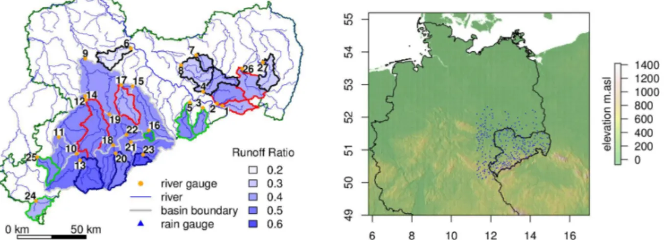
Fig. 2. Left panel: map of the study area and long term average basin runoff ratios of the basins investigated. The bold numbers depict the id (cf. Table 1) of the river gauges (orange dots). The colour of the basin boundary refers to the 4 basin groups as used in Fig. 6. Grey boundaries indicate that the respective basin does not belong to any of these groups. Right panel: simple topographic map (geographical coordinates) of northern Germany with hillshading and terrain colours depicting elevation (Jarvis et al., 2008). The borders of Germany and Saxony are drawn as black lines and rain gauges used for interpolation are shown as blue triangles.
description of these processing steps can be found in the ap-pendix. All procedures are based on monthly data, as the method to filter the annual periodic components of the time series does not need higher temporal resolution data.
Due to extensive hydraulic engineering projects since the industrial revolution in the 19th century, a dense network of hydrologic gauging stations has been established in Saxony. We have chosen 27 river gauge stations, which almost fully cover the period 1930–2009. The stations cover large parts of Saxony, with catchment areas ranging between 37 and 5442 km2. Most stations are within the Mulde River basin (15) or are tributaries of the Upper Elbe (6). Note that a range of basins are part of a common river network and are there-fore physically and statistically not independent. However, 18 out of 27 are head water basins, which can be regarded as independent in terms of watershed properties. Detailed information may be found in Table 1 and the map in Fig. 2.
The discharge data have been converted to areal monthly runoff (mm month−1) using the respective catchment area. Then the data have been subject to a homogeneity test proce-dure based on the catchments runoff ratio. Thereby, the Pet-titt homogeneity test (PetPet-titt, 1979) has been performed on annual data as well as in a seasonal setting, where for each calendar month the test statistic has been computed sepa-rately, but only the largest test statistic of all months has been taken for significance testing. The significance levels have been determined by a Monte-Carlo simulation with normal N(0, 1)distributed random numbers. The details of 7 sig-nificant (α= 0.05) inhomogeneous series are reported in Ta-ble 2. Note, that the reported year of the maximal test statis-tic does not necessarily identify the correct change point. However, in three cases dam constructions may be the prob-able cause of the inhomogeneity. For the other runoff series,
no obvious reason has been found for the detected inhomo-geneities. These are probably related to measurement errors (for example changes in the rating curve due to cross section changes) or the changes in catchment characteristics.
4 Results and discussion
4.1 Estimation and variability of the timing of the
runoff ratio
To gain some insight in the general spatial behaviour of the runoff ratio of the selected basins, a map of the long term av-erage runoff ratio is presented in Fig. 2. There is generally a higher runoff ratio in southern mountainous basins, having a runoff ratio up to 0.6, which is mainly due to higher precipita-tion (up to 1030 mm annually). The basins in the hilly North have lower runoff ratios ranging between 0.2 and 0.4 and are characterised by lower precipitation (down to 630 mm), higher evapotranspiration and in contrast to the higher basins, larger bodies of groundwater due to unconsolidated rock.
As an example, a time series of the runoff ratio is shown for the gauge at Lichtenwalde in Fig. 3. The three-monthly running runoff ratio shows a distinct seasonal pattern, while the 2-year running runoff ratio exhibits some low-frequency variability. Looking at the spectra of the runoff ratio series, two distinct peaks are generally found, one at an annual and the other at the half-year frequency (not shown).
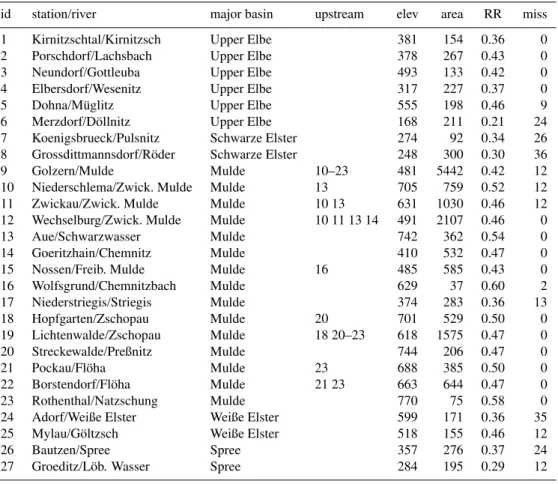
Table 1.River stations analysed over the period 1930–2009. The column elev denotes the mean basin elevation in meters above sea level, area denotes catchment area in km2, RR denotes the long term average runoff ratio and miss gives the number of missing months.
id station/river major basin upstream elev area RR miss
1 Kirnitzschtal/Kirnitzsch Upper Elbe 381 154 0.36 0
2 Porschdorf/Lachsbach Upper Elbe 378 267 0.43 0
3 Neundorf/Gottleuba Upper Elbe 493 133 0.42 0
4 Elbersdorf/Wesenitz Upper Elbe 317 227 0.37 0
5 Dohna/M¨uglitz Upper Elbe 555 198 0.46 9
6 Merzdorf/D¨ollnitz Upper Elbe 168 211 0.21 24
7 Koenigsbrueck/Pulsnitz Schwarze Elster 274 92 0.34 26
8 Grossdittmannsdorf/R¨oder Schwarze Elster 248 300 0.30 36
9 Golzern/Mulde Mulde 10–23 481 5442 0.42 12
10 Niederschlema/Zwick. Mulde Mulde 13 705 759 0.52 12
11 Zwickau/Zwick. Mulde Mulde 10 13 631 1030 0.46 12
12 Wechselburg/Zwick. Mulde Mulde 10 11 13 14 491 2107 0.46 0
13 Aue/Schwarzwasser Mulde 742 362 0.54 0
14 Goeritzhain/Chemnitz Mulde 410 532 0.47 0
15 Nossen/Freib. Mulde Mulde 16 485 585 0.43 0
16 Wolfsgrund/Chemnitzbach Mulde 629 37 0.60 2
17 Niederstriegis/Striegis Mulde 374 283 0.36 13
18 Hopfgarten/Zschopau Mulde 20 701 529 0.50 0
19 Lichtenwalde/Zschopau Mulde 18 20–23 618 1575 0.47 0
20 Streckewalde/Preßnitz Mulde 744 206 0.47 0
21 Pockau/Fl¨oha Mulde 23 688 385 0.50 0
22 Borstendorf/Fl¨oha Mulde 21 23 663 644 0.47 0
23 Rothenthal/Natzschung Mulde 770 75 0.58 0
24 Adorf/Weiße Elster Weiße Elster 599 171 0.36 35
25 Mylau/G¨oltzsch Weiße Elster 518 155 0.46 12
26 Bautzen/Spree Spree 357 276 0.37 24
27 Groeditz/L¨ob. Wasser Spree 284 195 0.29 12
Table 2.Results of homogeneity tests of runoff ratio and information of larger dam constructions with the respective volume of the reservoirs given in hectometres (hm3). The column Inhomogeneity reports the year and the month the maximal Pettitt test statistic and their respective significance levels.
Station Inhomogeneity Additional information
Streckewalde annual: 1952∗∗∗, seasonal: Jun 1970∗∗ dam construction 1973–1976, 55 hm3a Goeritzhain annual: 1953∗∗∗, seasonal: Apr 1959∗
Niederstriegis annual: 1962∗∗∗, seasonal: Apr 1957∗∗
Neundorf annual: 1967∗∗, seasonal: Mar 1976∗ dam construction 1976, 14 hm3b Groeditz annual: 1948∗, seasonal: Apr 1948∗
Pockau annual: 1980∗, dam construction 1967, 15 hm3c
Rothenthal seasonal: Feb 1981∗∗
∗α= 0.05,∗∗α= 0.01,∗∗∗α= 0.001.
ahttp://de.wikipedia.org/wiki/Talsperre Pre{\OT1\ss}nitz,bhttp://en.wikipedia.org/wiki/Gottleuba Dam,chttp://de.wikipedia.org/wiki/Talsperre Rauschenbach
of the monthly runoff ratio series are explained by this fit. However, as we are interested in the smooth seasonal signal, we used three-monthly running runoff ratios RR3to filter the
annual cycle. Between 71 and 84 % of the variability of RR3
is explained by the fitted cosines. Another positive effect is that the standard deviation of the annual phases estimated for
monthly runoff ratios decreased from 18.5–27.6 to 12.7–20.1 days, when using three-monthly moving runoff ratios. This is mainly due to less extreme years, while keeping the overall phase average (54.4 to 55.3).
runoff r
atio
, Q / P
1940 1960 1980 2000
0.2 0.4 0.6 0.8 1.0 1.2 1.4
3 − month MA 2 − year MA
Fig. 3. Time series of smoothed monthly runoff ratio at Lichten-walde, Zschopau.
computed. We find that there are no significant (α= 0.05) correlations in any series at lags from 1 to 10 years. Further the empirical distributions have been plotted vs. the “Von Mises” distribution (Jammalamadaka and Sengupta, 2001; Lund and Agostinelli, 2010), which showed no substantial deviations from the 1:1 line. The “Von Mises” distribution may be regarded as equivalent to the normal distribution for circular data. Thus, the timing estimates do not violate dis-tribution and independence assumptions for trend and corre-lation assessment.
Next, average characteristics of the timing of runoff ra-tio over Saxony are analysed. We already discussed that the runoff ratio shows a north to south gradient corresponding to increasing basin elevation (Fig. 2), which is confirmed by the left panel of Fig. 4, depicting the relationship between the runoff ratio and basin elevation. We find that the annual phase is even more dependent on the basin elevation, cf. the right panel of Fig. 4, with a strong linear relation of 5.5±0.3 days per 100 m elevation change. Naturally, lower basins ap-pear to have an earlier timing than higher basins, which is due to earlier snow melt in winter/spring.
To generalize the results and because of the strong link to altitude, we chose to group the basins according to their aver-age elevation, which resulted in 4 groups. For each group the phase average has been computed for each year using circular means (Eq. 4). Further, only non-connected basins are used, to achieve a set of independent basins. The respective height intervals and corresponding basins are presented in Table 3. Descriptive statistics such as circular average and standard deviations for each elevation group are given in columnφ¯RR.
As independent comparison to the annual phases estimated from RR3, the basin average half-flow date and its standard
deviation are shown in columnQ¯50 of Table 3. Generally,
the half flow dates appear later than the annual phase es-timates, with about 44 days in the lowest basin group and about 30 days in highest elevated basins. So half-flow dates do not show such a clear difference between high and low basins as annual phases do. Further, as lower basins do not have such a distinct seasonal pattern as higher basins, half
● ● ● ● ● ● ● ● ● ● ● ● ● ● ● ● ● ● ● ● ● ● ● ● ● ● ●
200 300 400 500 600 700
0.2
0.3
0.4
0.5
0.6
basin average elevation [m asl]
a ver age r unoff r atio [−] ● ● ● ● ● ● ● ● ● ● ● ● ● ● ● ● ● ● ● ● ● ● ● ● ● ● ● ● ● ● ● ● ● ● ● ● ● ● ● ● ● ● ● ● ● ● ● ● ● ● ● ● ● ●
200 300 400 500 600 700
40 45 50 55 60 65 70 75
basin average elevation [m asl]
a
ver
age streamflo
w timing [do
y] ● ● ● ● ● ● ● ● ● ● ● ● ● ● ● ● ● ● ● ● ● ● ● ● ● ● ●
Fig. 4. Height dependence of long term average runoff ratio (left panel) and dependence of the average streamflow timing (right panel).
flow dates are less able to discern the correct timing (D´ery et al., 2009).
Comparing the different measures using the timing aver-age for all series and years, the phase estimate for the runoff ratio is smallest (φRR= 55), while the half-flow dates are
largest (Q50= 93). However, if we compute the phase
di-rectly from monthly streamflow we yieldφQ= 70, which is in between. So a part of the differences found betweenQ50
andφRR are due to the fact that half-flow dates are based
solely on streamflow, while the phase estimate of the runoff ratio is normalised by precipitation. The other part of the dif-ferences is due to the different timing estimation techniques. There are also differences in standard deviationσ between both measures. WhileQ50 shows aσ of about 19 days, the
timing measure using runoff ratios has aσ of about 14 days. The larger variability inQ50 can probably be attributed to
larger uncertainties in its estimation, e.g. owing to single events (D´ery et al., 2009).
4.2 Temporal variability of the timing
As the timing estimate has been computed for each calen-der year, it is now possible to investigate the high and low-frequency temporal variability.
Figure 5 presents annual phase estimates (converted into doy) of the runoff ratio of the lowest and the highest basin group, respectively. In general, there is a natural difference in timing between lower basins and more mountainous basins. However, from Fig. 5 it is apparent that these differences changed over time with much larger differences in the pe-riod 1950 to 1980. Also the year-to-year variability ofφRR
is larger as well. In contrast to the low basins, there is a trend towards earlier timing in the higher basins since the late 1960s, decreasing the differences between low and high basins. We further note that the difference observed in the last two decades is now smaller than it has been observed before 1950. All other basins at medium elevations show a behaviour somewhere in between the both groups.
Table 3.Average statistics of the river gauge stations, grouped according to basin average elevation without connected basins. The columns denote in order of appearance: the respective elevation interval, group member basin id, the phase averageφ¯RR as calender day with
respective circular standard deviation in days, the average half-flow dateQ¯50, circular correlation coefficientsρccbetweenφRRandφT,
the linear regression coefficientTcoefand its standard deviation and the circular-linear correlationρsnowbetween snow depths in March and
φRR.
elevation id φ¯RR Q¯50 ρcc Tcoef ρsnow
160–320 4 6 7 8 27 11 Feb±14 28 Mar±19 0.23 0.93±0.45 0.53 360–420 1 2 14 17 26 14 Feb±14 29 Mar±19 0.31 1.27±0.45 0.64 500–620 3 5 16 24 25 25 Feb±13 1 Apr±20 0.55 2.01±0.34 0.50 740–780 13 20 23 11 Mar±16 10 Apr±18 0.59 2.64±0.41 0.72
phase as do
y
1940 1960 1980 2000
0
50
100
150 elevation interval 160 − 320 740 − 780
Fig. 5.Time series of the annual phase of runoff ratio for two groups of stations at high and low elevations, respectively. The shaded area shows the within group range and the bold lines depict the 11-year moving average of the group average annual phase.
streamflow in winter, especially in March, while decreasing discharge is observed from April to June. These trends imply a change in the phase of the cycle towards earlier timing of streamflow. So, considering the same period (1962–2004) as Stahl et al. (2010), we can confirm a decreasing trend in the phase of runoff ratio in mountainous basins, see Fig. 5.
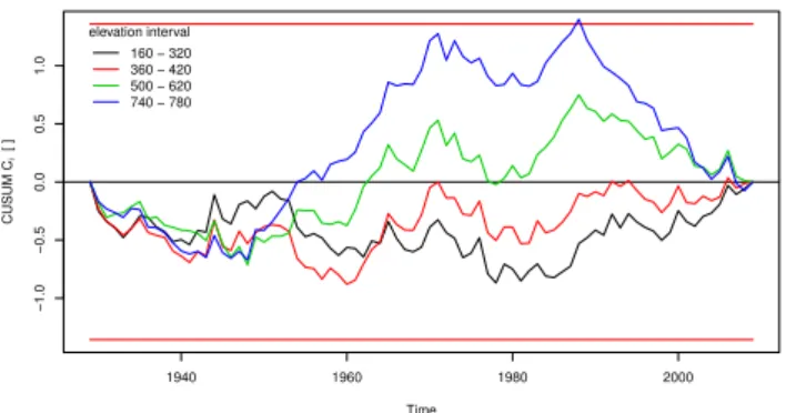
In the following, the decadal variability, trend patterns and change points of the timing of the runoff ratio will be anal-ysed. Since we did not expect a linear trend prevailing over this long period from 1930–2009, we chose to analyse the data using CUSUM graphs, which display the low-frequency variability and structural deviations from the long term aver-age over time. Figure 6 shows CUSUM lines based on the group average timing of the runoff ratio. The graph shows that with the beginning of the 1950s different trend directions in the particular basin groups have evolved. Basins above 500 m show upslope sections until 1971 and again from 1980 to 1988, exhibiting above average behaviour. This pattern is modulated by elevation and reveals that the low-frequency changes in timing are largest in the highest basins, where the CUSUM line hits theα= 0.05 significance level of a station-ary process in the year 1988. Another peak, although lower, is found in 1971. The peaks mark changes in trend directions
Time
CUSUM
Ci
[ ]
1940 1960 1980 2000
−1.0
−0.5
0.0
0.5
1.0
elevation interval 160 − 320 360 − 420 500 − 620 740 − 780
Fig. 6.CUSUM Analysis of the annual phase of runoff ratio. Basins have been grouped according to their altitude and then a group av-erage phase has been computed and used for the CUSUM analysis. The significance levels (α= 0.05) for a stationary process are de-noted as horizontal lines at the top and bottom of the graph.
and because they are positive, they reveal decreasing condi-tions. Both peaks are found in all CUSUM graphs, which is an indication that the low-frequency variability is mainly driven by a larger scale process.
Considering the year 1988 as a probable change point, the average shift in timing before (1950–1988) and after (1988– 2009) is assessed. While the lowest basins show a delay of 7 days, there is no shift in the second elevation group. The basins above 500 m show negative shifts, i.e. an earlier tim-ing of 10 and 22 days, respectively. Causes of the negative trend patterns will be discussed in the next subsections.
4.3 Does temperature explain trends in seasonality of runoff ratio?
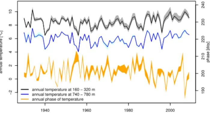
Having analysed the phase of the runoff ratio, it is interesting to check for direct links to climatic variables, especially tem-perature. In Fig. 7 time series of the annual average tempera-tures for the lowest and highest basin groups are shown. The depicted range is drawn from single basin temperature se-ries. The apparent temperature difference between the basin groups of about 2.5 K reflects the typical elevation gradient of temperature.
In the temperature series of basins at low elevations, a positive linear trend is detected in the order of 0.01 K per year (Kendall test p-value 0.02). Here, we applied the non-parametric trend test procedure for autocorrelated data sug-gested by Yue et al. (2002). In the higher basins the lin-ear trend is weaker with 0.003 K per ylin-ear (Kendall test p-value 0.22) and not significant. Instead, there is a period of lower temperatures from 1960 to 1990. Since then an in-crease is found.
The timing of the annual cycle of temperature for the basins investigated is also shown in Fig. 7. The differences between the basins are small (1.5 days between lowest and highest basins) compared to the standard deviation (on aver-age 3.5 days). The long term variability of the annual phase of temperature is relatively constant. However, since the end of the 1980s, there is a decline in the average of about 4 days, concluding with the most extreme years (2006 very late, and 2007 very early) observed.
To visualise the temperature timing influence on the sea-sonality of runoff ratio, we classified the 80 years of data into early years, having annual phases below the first quar-tile (before doy 198) and late years, having phases in the last quartile (after doy 204). Then we used this classification to bin the series of runoff ratio for every month over the year. The resulting boxplots in Fig. 8 depict the seasonal runoff ra-tio distribura-tion of each group over the year. As can be seen for the river gauge Koenigsbrueck, larger runoff ratios and larger variability from February to April are observed in late years, than in early years. At the river gauge Lichtenwalde, the differences between early and late years are even more distinct, with significant differences for the months April till August, with late years having an higher runoff ratio than earlier ones. The opposite is true for the months October till December. The average monthly temperatures superimposed in Fig. 8, reflect the actual differences between early and late years on temperature, which are larger during the first half of the year.
To quantify the link between these angular variables, cir-cular correlation coefficients have been computed from the annual phase of the basin runoff ratio and the annual phase of the basin average temperature. The results are detailed for each basin elevation group in Table 3, columnρcc. The
cor-relation coefficients tend to increase with elevation. A linear regression allows to assess the average effect of a change in
ann
ual temper
ature [°C]
1940 1960 1980 2000
−2
0
2
4
6
8
10
190
200
210
220
230
240
phase [do
y]
annual temperature at 160 − 320 m annual temperature at 740 − 780 m annual phase of temperature
Fig. 7. Range and mean of annual average temperatures of basins in the lowest and highest basin group. Orange shading: the range of annual phases of basin temperatureφT of all 27 basins (units on
right axis).
the phase of temperature on the timing of the runoff ratio. The slope coefficient and its standard deviation of the regres-sion line for each basin group is reported in Table 3, column
Tcoef. Note that in this case the timing has been treated as
linear variable. The coefficient is also plotted against av-erage basin elevation for all basins in Fig. 9. Again, there is a distinct height dependence, which is increasing with 0.36±0.01 per 100 m basin height. For mountainous basins, we find a coefficient of about three in magnitude, which means that a decrease of the phase of temperature of 5 days, amounts to a decrease of 15 days in the timing of the runoff ratio.
The increased sensitivity of hydrological regimes to tem-perature at higher altitudes has been often cited in literature. E.g. Barnett et al. (2005) state that rising temperatures possi-bly lead to earlier timing of the hydrologic regime. We find indeed that the annual basin temperature is correlated with the annual phase of runoff ratio. In fact, there is a linear-circular correlation of−0.37 in the highest basins, which is linearly increasing with decreasing basin elevation to 0.13 in the lowest basins. However, this correlation is only half in magnitude compared to the phase of temperature. Consider-ing the whole annual cycle, the timConsider-ing relationship between temperature and runoff ratio is stronger and more relevant than the one with annual temperatures.
4.4 Trend analysis in snow dominated basins
Jan Mar May Jul Sep Nov 0 1 2 3 runoff r
atio Q / P
Koenigsbrueck / Pulsnitz 275 m
0 1 2 3 early late −20 −10 0 10 20 temper ature [°C]
Jan Mar May Jul Sep Nov
0
1
2
3
runoff r
atio Q / P
Lichtenwalde / Zschopau 619 m
0 1 2 3 early late −20 −10 0 10 20 temper ature [°C]
Fig. 8. Box-whisker plots of monthly values of runoff ratio. The data are grouped according to early years with the annual phase of temperature below the 1st quartile and late years beyond the 3rd quartile. The bold grey and black lines denote the average monthly temperature for late and early years, with the corresponding axis on the right. The difference in temperature is shown as dashed line. The whiskers show the largest/lowest values within 1.5 – times of the interquartile range (IQR). Values outside 1.5×IQR, if any, are denoted as outliers and are not shown for display reasons. There are quite a few outliers, but these are equally distributed among the groups.
● ● ● ● ● ● ● ● ● ● ● ● ● ● ● ● ● ● ● ● ● ● ● ● ● ● ●
200 300 400 500 600 700
0
1
2
3
4
basin average elevation [m asl.]
slope phase RR vs
. phase T [da
y/da y] _ _ _ _ _ _ _ _ _ _ _ _ _ _ _ _ _ _ _ _ _ _ _ _ _ _ _ _ _ _ _ _ _ _ _ _ _ _ _ _ _ _ _ _ _ _ _ _ _ _ _ _ _ _
Fig. 9. Height dependence of the regression slope coefficient (±standard deviation) between annual phases of streamflow and temperature.
Winter average snow depths and snow cover are poorly correlated to the annual phase of runoff. For the basin Lichtenwalde and station data at Fichtelberg, ρc−l is not very high and also not significantly different from 0 at the
α= 0.05 level (ρc−l= 0.2 for winter average snow depths and
ρc−l= 0.29 for snow cover duration). However, the average snow depth in March appears to have a significant correlation (ρc−l= 0.55). Therefore, for each basin the March average snow depth has been computed. Regarding the basin groups, we found positive and significant correlations, that are largest in the highest basins, see also Table 3, columnρsnow.
Having identified the links of temperature, snow depth and runoff ratio in snow melt influenced basins, we investigated whether these variables might explain the trend patterns
Time
CUSUM
Ci
[ ]
1940 1960 1980 2000
−1.5 −1.0 −0.5 0.0 0.5 1.0 1.5
phase runoff ratio phase temperature march snow depth annual average temperature
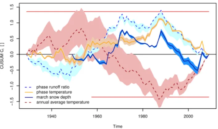
Fig. 10. CUSUM Analysis of the 3 highest head water basins sit-uated in the Ore Mountains. The bold lines denote the particular group average series, while the shaded areas depict the range of the single CUSUM lines. The significance levels (α= 0.05) for a sta-tionary process are denoted as horizontal lines at the top and bottom of the graph.
however, does not influence the general behaviour, with the negative peak in the year 1988, revealing a significant change in the mean towards higher temperatures. Also the phase of temperature shows a peak in 1988, but in opposite direction, indicating decreasing conditions. Besides, the low-frequency behaviour of the phase of temperature is not influenced by the change in station density, showing the robustness of this measure.
The CUSUM graph of the annual phase of runoff ratio (Fig. 10) also shows this peak in 1988, reaching the signifi-cance levelα= 0.05. Moreover, there is another peak appar-ent in 1971, where there is no indication from both temper-ature related series. But, we found a striking similarity of the CUSUM graph for March snow depths, which displays both peaks and even though the significance levels are not reached, they provide evidence, that late winter snow cover may also explain the low-frequency variability ofφRR.
These statistical links underline the strong influence of late winter snow cover on the timing ofφRRand subsequently on
the annual hydrological regime. This influence naturally in-creases with elevation (cf. columnρsnowof Table 3). Under
the assumption that there is no limitation of winter precipita-tion, snow cover is to a large part controlled by temperatures below or above 0◦C. This argument might be an explanation that with increasing basin elevation, also increasing correla-tion and linear slopes (cf. Fig. 9) have been found between the timing of temperature and the timing of the runoff ratio (cf. Table 3). Still, late winter snow cover is a better predictor than the phase of temperature.
The coincidence of peaks in the CUSUM graphs in Fig. 10 indicates that the respective elements undergo structural changes at the same time. Especially the apparent 1988 change point in all series investigated may be related to dis-tinct changes towards less air pollution with aerosols over CE since 1980 (Philipona et al., 2009). So probably, the in-creasing incoming short wave radiation resulted in increased temperatures, earlier snow melt and, eventually, also in the advance of the timing of temperature.
Air pollution also impacted forest vegetation, with sub-sequent tree-die off since the 1960s and with major clear cuts in the 1980s ( ˇSr´amek et al., 2008) at the mountain ridge in southern Saxony. Thus especially the headwaters of some rivers analysed here have been affected. Such dra-matic changes in vegetation cover may have also influenced hydrologic processes and subsequently the timing of runoff ratio. However, quantifying such effects is out of the scope of this study, and remains open for further research.
4.5 Uncertainty and significance of the results
For the interpretation of the results it is necessary to list the sources of uncertainty and to examine their relevance.
First of all, there may be measurement errors or inhomo-geneities in the observed runoff and rainfall series. When we assume that these errors lead to an abrupt but constant change
of the mean at a given location, the cyclic behaviour and thus the phase is unlikely to be affected systematically.
In 7 basins inhomogeneities in the runoff ratio series have been detected. Without detailed information, it is impossi-ble to correct for such changes. Therefore, these records have been kept in the dataset without a correction. We per-formed some cross checking by subsequently removing the suspect series from the computation of the group averages. The resulting differences to the original group average are of comparable magnitude than the standard deviation of the averaged series, but small with respect to the assessed corre-lations and long term shifts.
Another source of uncertainty is the estimation of basin precipitation. Apart from the spatial interpolation error, which is assumed to average out, we had to face the problem of changes of the observation network over time. To check for effects of this inhomogeneity, three different sets of in-put stations have been prepared (cf. the Appendix). When comparing the resulting annual phases of these different pre-cipitation input sets, only marginal differences for the timing estimates have been found.
Then there is some uncertainty in the estimation of the timing of the annual cycle using the approximation of a har-monic function to the data. We quantified this uncertainty by calculating the explained variance of the original series. This is not possible for traditional timing measures, such as half-flow dates. Further we showed that the year-to-year variabil-ity could be reduced by smoothing the data before applying the annual filter.
Finally, the overall uncertainty in the phase estimates and their low-frequency variability was assessed by grouping the data according to basin elevation. The range within a group is a measure of the accuracy of our estimates. As these ranges were generally smaller than the temporal variability, we can conclude that the averaging method was robust. Moreover, the main features are repeated within this large set of river basins distributed over several elevation levels. This last ar-gument underlines that the change points found in the phase of runoff ratio are not random or catchment specific, but a result of changing climate conditions.
5 Conclusions
deviation of the harmonic measure is generally lower and thus less influenced by single events.
A climatology of the timing of the dimensionless runoff ratio (RR) was established, covering 27 river basin at dif-ferent elevation levels. Basin elevation was found to be the most important catchment characteristic, controlling (i) av-erage timing, (ii) the magnitude of observed long-term shifts in timing and (iii) the apparent sensitivity to the timing of temperature. All mentioned characteristics increase with el-evation.
Analysing the temporal variability, we observed a shift of the seasonal cycle towards occurring earlier in the year in basins being on average above 500 m, with the largest changes in the highest basins. This long-term shift in tim-ing of runoff ratio represents a trend towards earlier timtim-ing of about 10 to 22 days in the last two decades, relative to the prevailing conditions between 1950 and 1988.
The interannual variability of runoff ratio timing records is in the same order as the apparent long term shifts, but independent from elevation. There is, however, a remark-able coherence of the year-to-year changes across all basins analysed. Also, the long-term change patterns revealed by a CUSUM analysis of the standardised anomalies showed a similarity in slopes and peaks between elevation groups. Presumably, the observed changes are driven by larger scale physical processes, which have similar effects at the annual, as well as at the decadal time scale.
As expected, a large fraction of the observed variability may be explained by the low and high frequency variability of temperature records. Indeed, the annual timing of temper-ature, which can be estimated with high confidence, showed significant positive correlations with the timing of the runoff ratio. Again, the correlation as well as the linear regression coefficient showed to be dependent on basin elevation. More-over, the timing of the temperature cycle has more influence on the timing of the runoff ratio than the magnitude of annual average temperatures.
However, the apparent low-frequency variability of RR could not be explained by temperature observations alone. The main cause of the observed high and low frequency vari-ability in higher elevated basins is the varivari-ability of late win-ter snow cover. It explained a larger fraction of the variability than the timing of temperature and matched the low frequent departures from the average of the timing of runoff ratio quite well.
The climatic changes observed by the temperature regime are most likely the major cause of the observed changes in hydrological variables. There is evidence of a structural change of the average behaviour of several observation vari-ables in the year 1988. The CUSUM related stationarity test revealed (i) a significant shift in the timing of runoff ratio in high basins, (ii) a marked but not significant change in late winter snow depths, accompanied by (iii) a significant in-crease of annual temperature of about 1 K and (iv) a marked
but not significant advance of the timing of temperature of 4 days.
We believe that this chain of changes has been triggered by the drastic changes in industrial and domestic air pollution, because the dimming and brightening of the atmosphere over Saxony resulted in remarkable changes in solar insolation. Further, this accelerated and distinct change in the timing of both, temperature and runoff ratio indicates that impacts of climate change on the water cycle are stronger in mountain-ous areas.
If the trends in the phase and average of temperature per-sist, a range of potential problems for water resources man-agement will evolve. The most critical problem is that the de-lay between natural water supply and demand will increase and subsequently a larger artificial storage volume may be needed to maintain the same security level of supply. Next, the shift in both, mean and variability of monthly streamflow will alter traditional assumptions used for predicting seasonal water availability. This underlines the importance for main-taining and improving the existing observational network.
Appendix A
Preparation of basin input data
A1 Precipitation
The geographical domain (11.5◦–16◦E, 50◦–52◦N) has been chosen for the spatial interpolation and station data selection. The station network density has changed dramatically throughout time. Currently there is one station available in the database since 1858, 12 stations since 1891 rising up to 111 in the 1930s. Due to World War II only 20 stations were available in 1945. From the 1950s, the network has improved from 374 in 1951 to a maximum of 873 in 1990. Since 2000, the network density decreased to 354 in 2008.
To check for influences of the changing network, three data sets have been prepared. One set only with stations cov-ering the full period without longer missing periods, another set which consists of all observations available at a time step and another set which has been used in the analysis. This last set is a compromise between the other two sets, meeting the requirement that the respective series covers at least 40 years, i.e. from 1950–1990. This set contains 368 stations.
previous test, (ii) best correlation of the differenced series (Peterson and Easterling, 1994), (iii) cover most of the record of the candidate station and (iv) are close to the candidate. Then the Alexandersson homogeneity test and the Pettitt test have been applied. If both tests reject the hypothesis of sta-tionarity at theα= 0.01 level, then the series has been flagged as suspect. Finally, a set of 299 precipitation series have been left for spatial interpolation, i.e. without any suspect series. The stations can be found in the right panel of Fig. 2. There are 83 stations during the 1930s, about 290 from 1950–1990 with 170 in the last decade.
Based on the station dataset a spatial interpolation for each month has been computed. First, a linear height relation-ship using a robust median based regression (Theil, 1950) has been established. Then the residuals have been inter-polated onto an aggregated SRTM grid (Jarvis et al., 2008) of 1500 m raster size using an automatic Ordinary Kriging (OK) procedure (Hiemstra et al., 2009). Monthly basin av-erage precipitation is then computed by the avav-erage of the respective grid cells. The method of height regression and OK of the residuals has been chosen, as this method showed to have the lowest root-mean-square errors (RMSE) among other methods in a cross-validation based on monthly station data sets.
A2 Temperature and snow depth data
The network of climate stations in the domain has also changed during time. Since 1930, 9 long temperature se-ries have been available, this increased to 47 in 1961 and again reduced to 38 in 2008. A few snow depth observations are available from climate stations. Additionally, a dense network of snow depths has been established in the region since 1950. On average, 163 series are available. For both elements, the basin averages have been computed using the methods already described for precipitation in Sect. A1. Acknowledgement. This work was kindly supported by Helmholtz Impulse and Networking Fund through Helmholtz Interdisci-plinary Graduate School for Environmental Research (HIGRADE) (Bissinger and Kolditz, 2008). We further acknowledge LfULG for providing the runoff time series and the German Weather Service (DWD), Czech Hydro-meteorological Service (CHMI) for provid-ing climate data. Micha Werner (UNESCO-IHE), Klemens Barfus and Kristina Brust (TU Dresden) are gratefully acknowledged for reading and correcting the manuscript. Boris Orlowsky (reviewer), two anonymous reviewers and Bart van den Hurk (editor) greatly helped to improve the manuscript.
Edited by: B. van den Hurk
References
Barnett, T., Adam, J., and Lettenmaier, D.: Potential impacts of a warming climate on water availability in snow-dominated re-gions, Nature, 438, 303–309, 2005.
Bernhofer, C., Goldberg, V., Franke, J., H¨antzschel, J., Harmansa, S., Pluntke, T., Geidel, K., Surke, M., Prasse, H., Freydank, E., H¨ansel, S., Mellentin, U., and K¨uchler, W.: Sachsen im Klimawandel, Eine Analyse, S¨achsisches Staats-Ministerium f¨ur Umwelt und Landwirtschaft (Hrsg.), p.211, 2008.
Bissinger, V. and Kolditz, O.: Helmholtz Interdisciplinary Graduate School for Environmental Research (HIGRADE), GAIA-Ecol. Persp. Sci. Soc., 17, 71–73, 2008.
Brown, R., Durbin, J., and Evans, J.: Techniques for testing the con-stancy of regression relationships over time, J. Roy. Stat. Soc. B, 37, 149–192, 1975.
Court, A.: Measures of Streamflow Timing, J. Geophys. Res. 67, 4335–4339, doi:10.1029/JZ067i011p04335, 1962.
D´ery, S., Stahl, K., Moore, R., Whitfield, P., Menounos, B., and Burford, J.: Detection of runoff timing changes in pluvial, ni-val, and glacial rivers of western Canada, Water Resour. Res. 45, W04426, doi:10.1029/2008WR006975, 2009.
Dose, V. and Menzel, A.: Bayesian analysis of climate change im-pacts in phenology, Global Change Biol., 10, 259–272, 2004. Fanta, J.: Rehabilitating degraded forests in Central Europe into
self-sustaining forest ecosystems, Ecol. Eng., 8, 289–297, 1997. Fiala, T.: Statistical characteristics and trends of mean annual and monthly discharges of Czech rivers in the period 1961-2005, J. Hydrol. Hydromech., 56, 133–140, 2008.
Franke, J., Goldberg, V., and Bernhofer, C.: Sachsen im Klimawan-del Ein Statusbericht, Wissenschaftliche Zeitschrift der TU Dres-den, 58, 32–38, 2009.
Hiemstra, P., Pebesma, E., Twenh¨ofel, C., and Heuvelink, G.: Real-time automatic interpolation of ambient gamma dose rates from the dutch radioactivity monitoring network, Comput. Geosci., 35, 1711–1721, 2009.
Hodgkins, G., Dudley, R., and Huntington, T.: Changes in the tim-ing of high river flows in New England over the 20th century, J. Hydrol., 278, 244–252, 2003.
Huybers, P. and Curry, W.: Links between annual, Milankovitch and continuum temperature variability, Nature, 441, 329–332, 2006. Jammalamadaka, S. and Sengupta, A.: Topics in circular statistics,
World Scientific Pub Co Inc, 2001.
Jarvis, A., Reuter, H., Nelson, E., and Guevara, E.: Hole-filled seamless SRTM data version 4, International Center for Tropical Agriculture (CIAT). Available at: http://srtm.csi.cgiar.org (last access: 10 January 2011), 2008.
Kleiber, C. and Zeileis, A.: Applied econometrics with R, 1. edition, Springer Verlag, New York, USA, 2008.
KLIWA: Langzeitverhalten der mittleren Abfl¨usse in Baden-W¨urttemberg und Bayern, Institut f¨ur Wasserwirtschaft und Kul-turtechnik (Karlsruhe). Abteilung Hydrologie, Mannheim, http:// www.kliwa.de/download/KLIWAHeft3.pdf (last access: 10 Jan-uary 2011), 2003.
Loucks, D., van Beek, E., Stedinger, J., Dijkman, J., and Villars, M.: Water Resources Systems Planning and Management: An Introduction to Methods, Models and Applications, UNESCO, Paris, 2005.
Lund, U. and Agostinelli, C.: circular: Circular Statistics, http: //CRAN.R-project.org/package=circular, R package version 0.4 (last access: 10 January 2011), 2010.
Mote, P., Hamlet, A., Clark, M., and Lettenmaier, D.: Declining mountain snowpack in western North America, B. Am. Meteo-rol. Soc., 86, 39–49, 2005.
Paluˇs, M., Novotn´a, D., and Tichavsk`y, P.: Shifts of seasons at the European mid-latitudes: Natural fluctuations correlated with the North Atlantic Oscillation, Geophys. Res. Lett, 32, L12805, doi:10.1029/2005GL022838, 2005.
Peterson, T. and Easterling, D.: Creation of homogeneous compos-ite climatological reference series, Int. J. Climatol., 14, 671–679, 1994.
Pettitt, A.: A non-parametric approach to the change-point problem, Appl. Stat., 28, 126–135, 1979.
Philipona, R., Behrens, K., and Ruckstuhl, C.: How declin-ing aerosols and risdeclin-ing greenhouse gases forced rapid warmdeclin-ing in Europe since the 1980s, Geophys. Res. Lett., 36, L02806, doi:10.1029/2008GL036350, 2009.
Qian, C., Fu, C., Wu, Z., and Yan, Z.: The role of changes in the annual cycle in earlier onset of climatic spring in northern China, Adv. Atmos. Sci., 28, 284–296, 2011.
R Development Core Team: R: A Language and Environment for Statistical Computing, R Foundation for Statistical Computing, Vienna, Austria, http://www.R-project.org/, last access: 10 Jan-uary 2011, ISBN 3-900051-07-0, 2010.
Regonda, S., Rajagopalan, B., Clark, M., and Pitlick, J.: Seasonal cycle shifts in hydroclimatology over the western United States, J. Climate, 18, 372–384, 2005.
Stahl, K., Hisdal, H., Hannaford, J., Tallaksen, L. M., van Lanen, H. A. J., Sauquet, E., Demuth, S., Fendekova, M., and J´odar, J.: Streamflow trends in Europe: evidence from a dataset of near-natural catchments, Hydrol. Earth Syst. Sci., 14, 2367–2382, doi:10.5194/hess-14-2367-2010, 2010.
Stewart, I., Cayan, D., and Dettinger, M.: Changes toward earlier streamflow timing across western North America, Journal of Cli-mate, 18, 1136–1155, 2005.
Stine, A., Huybers, P., and Fung, I.: Changes in the phase of the an-nual cycle of surface temperature, Nature, 457, 435–440, 2009. ˇSr´amek, V., Slodiˇc´ak, M., Lomsk`y, B., Balcar, V., Kulhav`y, J.,
Hadaˇs, P., Pulkr´ab, K., ˇSiˇs´ak, L., Pˇeniˇcka, L., and Sloup, M.: The Ore Mountains: Will successive recovery of forests from lethal disease be successful, Mountain Research and Development, 28, 216–221, 2008.
Theil, H.: A rank-invariant method of linear and polynomial regres-sion analysis, (Parts 1–3), Nederlandse Akademie Wetenchappen Series A, 53, 386–392, 1950.
Thompson, R.: A time-series analysis of the changing seasonality of precipitation in the British Isles and neighbouring areas, J. Hydrol., 224, 169–183, 1999.
Thomson, D.: The seasons, global temperature, and precession, Sci-ence, 268, 59–68, 1995.
Vecchio, A., Capparelli, V., and Carbone, V.: The complex dy-namics of the seasonal component of USA’s surface temperature, Atmos. Chem. Phys., 10, 9657–9665, doi:10.5194/acp-10-9657-2010, 2010.
West, M. and Harrison, J.: Bayesian forecasting and dynamic mod-els, 2nd edition, Springer Verlag, New York, USA, 1997. Wild, M., Gilgen, H., Roesch, A., Ohmura, A., Long, C., Dutton,
E., Forgan, B., Kallis, A., Russak, V., and Tsvetkov, A.: From dimming to brightening: decadal changes in solar radiation at Earth’s surface, Science, 308, 847, 2005.
Yue, S., Pilon, P., Phinney, B., and Cavadias, G.: The influence of autocorrelation on the ability to detect trend in hydrological series, Hydrol. Process., 16, 1807–1829, 2002.
Zeileis, A. and Hornik, K.: Generalized M-fluctuation tests for pa-rameter instability, Statistica Neerlandica, 61, 488–508, 2007. Zeileis, A., Leisch, F., Hornik, K., and Kleiber, C.: strucchange: An