A Cross-Lingual Similarity Measure for
Detecting Biomedical Term Translations
Danushka Bollegala1*, Georgios Kontonatsios2,3, Sophia Ananiadou2,3
1Department of Computer Science, University of Liverpool, United Kingdom,2School of Computer Science, University of Manchester, Manchester, United Kingdom,3National Centre for Text Mining, University of Manchester, Manchester, United Kingdom
*danushka.bollegala@liverpool.ac.uk
Abstract
Bilingual dictionaries for technical terms such as biomedical terms are an important re-source for machine translation systems as well as for humans who would like to understand a concept described in a foreign language. Often a biomedical term is first proposed in En-glish and later it is manually translated to other languages. Despite the fact that there are large monolingual lexicons of biomedical terms, only a fraction of those term lexicons are translated to other languages. Manually compiling large-scale bilingual dictionaries for tech-nical domains is a challenging task because it is difficult to find a sufficiently large number of bilingual experts. We propose a cross-lingual similarity measure for detecting most similar translation candidates for a biomedical term specified in one language (source) from anoth-er language (target). Specifically, a biomedical tanoth-erm in a language is represented using two types of features: (a)intrinsic featuresthat consist of character n-grams extracted from the term under consideration, and (b)extrinsic featuresthat consist of unigrams and bigrams extracted from the contextual windows surrounding the term under consideration. We pro-pose a cross-lingual similarity measure using each of those feature types. First, to reduce the dimensionality of the feature space in each language, we proposeprototype vector pro-jection(PVP)—a non-negative lower-dimensional vector projection method. Second, we propose a method to learn a mapping between the feature spaces in the source and target language usingpartial least squares regression(PLSR). The proposed method requires only a small number of training instances to learn a cross-lingual similarity measure. The proposed PVP method outperforms popular dimensionality reduction methods such as the singular value decomposition (SVD) and non-negative matrix factorization (NMF) in a near-est neighbor prediction task. Moreover, our experimental results covering several language pairs such as English–French, English–Spanish, English–Greek, and English–Japanese show that the proposed method outperforms several other feature projection methods in biomedical term translation prediction tasks.
a11111
OPEN ACCESS
Citation:Bollegala D, Kontonatsios G, Ananiadou S (2015) A Cross-Lingual Similarity Measure for Detecting Biomedical Term Translations. PLoS ONE 10(6): e0126196. doi:10.1371/journal.pone.0126196
Academic Editor:Neil R. Smalheiser, University of Illinois-Chicago, UNITED STATES
Received:December 15, 2014
Accepted:March 30, 2015
Published:June 1, 2015
Copyright:© 2015 Bollegala et al. This is an open access article distributed under the terms of the
Creative Commons Attribution License, which permits unrestricted use, distribution, and reproduction in any medium, provided the original author and source are credited.
Data Availability Statement:The data has been uploaded as supplementary material to the system.
Funding:SA and GK acknowledge support from the UK Medical Research Council MR/L01078X/1 Supporting Evidence-based Public Health Interventions using Text Mining and AHRC AH/ L00982X/1, Mining the History of Medicine. The funders had no role in study design, data collection and analysis, decision to publish, or preparation of the manuscript.
Introduction
Technical terms are coined in many domain on a daily basis. In specialized domains such as medicine, technical terms are often first proposed in English and later translated into other lan-guages. Finding proper translations for technical terms is an important factor that expedites the technical knowledge across languages. Therefore, bilingual dictionaries for technical terms play an important role in both manual [1] and machine translation [2] approaches. Unfortu-nately, only a small fraction of the technical terms proposed in English are translated into other languages, which is problematic for machine translation systems that require bilingual term lexicons. For example, Unified Medical Language System (UMLS) Metathesaurus (http:// nlm.nih.gov/research/umls), one of the comprehensive multilingual medical resources cover-ing 21 languages, contains 75.1% English terms, 9.99% Spanish terms, 2.22% Japanese terms, and 1.82% French terms. The unbalanced representation of languages other than English in UMLS demonstrates the severity of the problem of technical term translation.
Manual translation of technical terms is a challenging task due to several reasons. First, it is difficult to find bilingual experts in highly technical domains who are willing to manually translate technical terms from one language to another. Second, domains such as medicine are so vast that it is difficult to find enough bilingual experts to cover all sub-domains within a do-main. Therefore, technical terms in some sub-domain within a large domain might not be suf-ficiently translated to other languages. Third, it is often difficult for humans to construct new translations from scratch although it is relatively easier to determine whether two words are suitable translations of each other. As a practical solution to this problem, we could assist human translators by providing a short list of translation candidates for a given technical term, thereby minimizing their effort to go through large term lexicons. Dictionaries and bilingual terminological resources are quickly out-of-date by the moment they are compiled due to the number of publications appearing in specialized domains such as medicine. Therefore, auto-matic methods for detecting translations for technical terms are important from the perspec-tive of update and maintenance.
In this paper, we model the problem of detecting translations of technical terms as a cross-lingual similarity measurement task [3]. Specifically, given a termwSin a source languageS,
and a termwTin a target languageT, we propose a cross-lingual similarity measure, sim(wS,
wT), that indicates the semantic similarity between the two termswSandwT. Throughout this
paper, we usetermto refer to single words or multi-word expressions that are used as technical terms in a particular field. We represent each termwin a languageL(which could be eitherS
orT) using two types of features: (a) character n-grams extracted fromw, and (b) contextual
extracted using an external corpus. We experimentally evaluate the effect of those two feature spaces for computing cross-lingual similarity.
Although two termswSandwTcould be represented using various features as described in
the previous paragraph, the two feature representations created for different languages will have low overlap in practice. For example, consider the English source and Japanese target lan-guage setting. The two lanlan-guages use different alphabets. Therefore, character n-gram features extracted for terms in English and Japanese languages will have no overlap. Likewise, contextu-al features are contextu-also less likely to overlap. Therefore, popular similarity measures such as the co-sine similarity between two feature vectors representing the two terms would often return zero similarity scores. To overcome this problem, we first learn a projection from the source lan-guage feature space to the target lanlan-guage feature space. Specifically, we model the projection learning problem as a multi-variate regression problem and use Partial Least Squares Regres-sion (PLSR) [4] to learn a projectionMfrom the source to the target language feature space. Next, we project the feature vectorwSfor the source termwSto the target language feature
space using the learnt projection. Let us denote the projection operation byM(wS). We train a
binary Random Forest (RF) classifier [5] to classify word pairs (wS,wT) depending on whether
wTis the correct translation ofwS. We represent a word pair (wS,wT) by a feature vector [wS;
wT;M(wS)], where we concatenate the three vectorswS,wT, andM(wS). Finally, the similarity
sim(wS,wT) between the source termwSand each of the target termswTis computed as the
class conditional probability returned by the random forest classifier expressing the likelihood ofwTbeing the correct translation ofwS. We rank the target language termswTin the
descend-ing order of their similarity scores to the source termwS, and display the top-ranked terms as
the potential translation candidates forwS. A human annotator can then pick the best
transla-tion(s) from this short-listed candidates set.
An important challenge when learning a projection between high dimensional feature spaces such as character n-grams or contextual features is that the number of parameters in the projection model tends to be large. In practice, to accurately learn this large number of parame-ters in a feature projection model we would require a large training dataset. However, this could be a problem in bilingual term translation because, the number of terms that are already translated between two languages are likely to be small, which prompts for automatic methods for detecting term translations in the first place. Therefore, it is desirable to design automatic term translation methods that can learn from a small number of training instances. For this purpose, we propose Prototype Vector Projection (PVP), a dimensionality reduction method to first project the source and target feature vectors to a lower-dimensional space. The Proto-type Vector Projection first selects a set ofd prototype vectorsfrom the feature vectors (n> >d
in total) representing terms in a language. We propose a method for selecting prototype vectors based on the number of non-zero elements in feature vectors. Each feature vector is then pro-jected to ad-dimensional space by taking the inner product with each of the prototype vectors. We finally learn a projection from the source to the target languages in this lower dimensional spaces using partial least squares regression (PLSR). PVP has several attractive properties such as: (a) the projections are always non-negative, given that the feature vectors are non-negative, (b) it does not require computationally expensive operations such as the Singular Value De-composition (SVD), and (c) the basis vectors (prototypes) are always actual data points, which make the interpretation of the lower-dimensional space easier.
to the rank R as the evaluation measure. Precision@R is a popular evaluation measure in infor-mation retrieval where it is considered desirable to rank relevant search results among the top ranked documents to a query. We compare PVP against several widely used dimensionality re-duction methods such as SVD or non-negative matrix factorization (NMF) using two synthetic datasets. PVP outperforms those methods in its ability to preserve the relative ranking of the nearest neighbors in the original space in the embedded space. Moreover, our experimental re-sults in a cross-lingual biomedical term translation detection task show that PVP outperforms SVD and NMF on both character n-gram features as well as contextual features for different language pairs.
Related Work
Measuring similarity between words and texts [6–8] is a fundamental task in Natural Language Processing (NLP) that is required for numerous other tasks such as document/word clustering [9], information retrieval [10–12], query suggestion [13], and word sense disambiguation [14]. A typical approach for measuring the similarity between two words is to first represent each word using the distribution of other words that co-occur with it in a corpus. The co-occur-rences could be weighted using a suitable word association measure such as the pointwise mu-tual information. Next, the similarity between two words is computed using a linear algebraic operation over the vectors such as their inner-product. Although this procedure for measuring similarity between words has been highly successful for measuring the similarity between words in the same language, it fails in the cross-lingual setting because, the distributional vec-tors that represent words in different languages have minimal or no overlap [15]. Therefore, we must project the feature spaces for each language into some common sub-space before we can compute the similarity between words selected from two different languages.
In cross-lingual latent semantic indexing [16], Singular Value Decomposition (SVD) is per-formed on a set of parallel texts such as the Hansard collection, which is written both in English and French. Documents are represented using a matrix where each row corresponds to a pair of parallel documents, and each column represents a word in source or target languages. The SVD step reduces the number of columns, thereby embedding words that are distributed simi-larly in the two languages in the same latent dimension. However, this method requires a col-lection of parallel texts, which is problematic in our setting of biomedical term translation using monolingual lexicons. The manual effort required to translate biomedical documents such as scientific papers to create parallel corpora is significantly larger compared to manually translating a set of biomedical terms. Considering that most machine translation methods re-quire either parallel or comparable corpora to train from, this rere-quirement rules out the appli-cability of such methods to the problem-setting we consider in this paper.
approaches for term translation depends heavily on the coverage of the bilingual seed dictio-nary that is used for translating lexical or sub-lexical basic units. For example, it has been re-ported that as much as 30% of incorrectly translated terms by such compositional methods are due to the poor coverage of the seed dictionary [22].
Kontonatsios et al. [23] proposed a binary classification approach for detecting biomedical term translations. They represent biomedical terms using character n-grams extracted from the terms and train a binary random forest classifier [5]. A manually annotated set of term pairs selected from the source and the target languages is used as the positive training instances, whereas the negative training instances are created by randomly pairing two terms from each language. They evaluate the performance of their method using two language pairs: English-French and English-Chinese. They use a balanced dataset that contains equal numbers of posi-tive and negaposi-tive (i.e. correct vs. incorrect translations) word pairs, and use classification accu-racy as the performance measure. However, in practice, we have only a handful of correct translations for a biomedical term although there will be many incorrect translations. There-fore, the balanced dataset approach does not reflect the true performance of a translation detec-tion method when used in real-world systems such as, to suggest transladetec-tion candidates to human annotators. Moreover, they do not consider contextual features, nor do they learn a mapping between the feature spaces corresponding to the two languages.
A bilingual dictionary-based approach for translating feature spaces between two languages to improve the accuracy of the cross-lingual similarity measurement is proposed by Kontonat-sios et al. in [24]. They use both character n-grams as well as contextual features to represent terms in a language. Contextual features are translated by looking them up in a bilingual dictio-nary. Unlike technical terms that have unambiguous translations, contextual features consist of common words that can be ambiguous and are difficult to translate without considering their context. Therefore, using a bilingual dictionary to translate contextual features would introduce additional noise to the term translation detection process. Moreover, the requirement for an additional bilingual dictionary besides the train word pairs could be problematic for resource poor languages.
Measuring cross-lingual lexical similarity has been studied in the cross-lingual information retrieval and the machine translation communities [25,26]. One line of approaches is to create cross-lingual topic models using parallel or comparable corpora such that words that express similar meaning in different languages are allocated to the same topic. Next, the similarity be-tween two documents or words in the two languages can be computed using the posterior probabilities over the learnt topics. Numerous techniques can be used to learn cross-lingual topic models such as non-negative matrix factorization [27,28], probabilistic principal compo-nent analysis [29], matching canonical correlation analysis [30], and multilingual probabilistic topic models [31,32].
Cross-lingual Term Similarity
Problem Definition
Given a list of termsQSin a source languageS, and a list of termsQTin a target languageT, we
consider the problem of finding one or more translations for each termwS2QSfrom the
tar-get term listQT. We assume the availability of a small seed list of term pairs {(wS,wT)} for
learning a cross-lingual similarity measure, sim(wS,wT), that indicates the degree of similarity
betweenwSandwT.
The trained cross-lingual similarity measure is used as follows. For each source termwS, we
measure its similarity to each of the target termswT, and rank the target terms in the
descend-ing order of their similarity scores sim(wS,wT). We display the topNranked candidates to a
human annotator to assist the process of finding term translations.
Two main approaches can be used to obtain a set of train term pairs {(wS,wT)} required by
the proposed method. First, we can use monolingual term extraction methods [18,34] to ex-tract two separate term lists for the source and target languages. For example, Xu et al. [35] pro-posed a language-independent method for extracting large collections of medical terms from semi-structured information sources on the Web. Next, a human annotator can manually align some of the words in the source term lexicon to their correct translations in the target term lex-icon. Obviously, there is no guarantee that all the terms found in the source term lexicon will have a corresponding translation in the target language lexicon. However, it is relatively easier for human annotators to find a translation for a given source language term from a list of can-didate target language terms than to come up with a translation by themselves, without having access to a target language term lexicon.
An alternative second approach would be to use bilingual lexicon extraction methods [36–
38]. These methods rely on comparable corpora such as Wikipedia articles written in different languages on the same topic or news articles published in different language on the same news event to measure similarity between terms written in different languages. One important prob-lem that needs to be addressed is the ambiguity of translations because a single source term can be translated to multiple different target language terms. For example, Bouamor et al. [37] use WordNet to disambiguate contextual vectors when measuring cross-lingual distributional sim-ilarity. Compared to the first approach, which requires a human to manually align two mono-lingual term lexicons, the second approach is attractive because it enables us to obtain a large bilingual term lexicon for a relatively lower cost. If we would like to further improve the quality of the train term pairs, then we can perform manual filtering on top of the automatically ex-tracted bilingual term lexicon.
Extracting train term pairs is beyond the scope of the current paper. In the subsequent dis-cussion, we assume the availability of such a train dataset, without attempting to extract it from comparable corpora. More importantly, our proposed method for learning a cross-lingual sim-ilarity measure does not assume any specific properties for the methods used for extracting train term pairs. Therefore, in principle the proposed cross-lingual similarity measure can be used to align term lists extracted from any term extraction method.
Monolingual Feature Vector Construction
The first step in our proposed method is to represent a term using a feature vector extracted from one of the source or the target languages. We refer to this step as themonolingual feature
vector constructionbecause the features we extract to represent a termwin a languageL
• Character n-gram Features:
We extract character n-grams for n = 2, 3, 4, and 5 from the termwas features. We then count the frequency of each n-gram extracted from all the terms in the training data, and se-lect the most frequent n-grams. In our experiments, we consider several n-gram feature spaces consisting of different numbers of n-gram features. Character n-grams can express different semantic information in different languages. For example, in phonetic languages such as English, French, Spanish, or Greek, character n-grams can capture the inflections or etymological components in the terms. On the other hand, in pictorial languages such as Jap-anese or Chinese, a singlekanjicharacter encodes rich semantics regarding the term such as its semantic compositionality. We refer character n-grams asintrinsicfeatures in this paper because they are extracted from the terms only, without requiring any external resources such as corpora, other than the term lexicons for the source and the target languages. We set binary feature values for the character n-grams extracted from a term. For example, consider the English termcatecholamine. Some of the character n-grams extracted from this term are (n= 2)ca, at, te, (n= 3)cat, ate, tec, (n= 4)cate, atec, tech, and (n= 5)catec, atech, techo.
• Contextual Features:
Although character n-grams are useful as intrinsic features for term alignment, they do not provide any information as to how those terms are used in a particular context. The distribu-tional hypothesis, often succinctly expressed using the memorable quote from Firth [39]– “you shall know a word by the company it keeps”, states that we can obtain useful insights into the semantics of a term by looking into the contexts in which that term appear in a cor-pus. We consider all occurrences of a termwin a corpus, and extract unigrams and bigrams of tokens that appear within a 5-token window surrounding the termw. Specifically, the two tokens preceding and the two tokens succeeding a term are considered as its contextual win-dow. In our experiments, we used the freely available Wikipedia (https://www.wikipedia.org/
) corpus for extracting contextual features.
For each extracted contextual feature we count the number of different train terms from which it is extracted. We then select the most frequent contextual features for representing terms. In our experiments we select the most frequent 10,000 contextual features from the source and the target languages. We set the value of a contextual featurecextracted for a termwto the positive pointwise mutual information (PPMI) [40]. PPMI is computed as
PPMIðc;wÞ ¼max 0;log pðc;wÞ
pðcÞpðwÞ
; ð1Þ
wherep(c),p(w) respectively denote the marginal probabilities of the contextual featurecand the termw, andp(c,w) denotes their joint probability. Note that the logarithmic term inEq 1
can become negative if the joint probability ofcandw(i.e.p(c,w)) is lesser than what would be expected ifcandwwere mutually exclusive (i.e.p(c)p(w)). This negative association of words is a result of incorrect probability estimates and is removed by setting to zero in the PPMI formula. We estimate those probabilities using the number of contexts in whichcand
wco-occur in the corpus as follows
pðcÞ ¼ no: of contexts in which coccurs
total no: of contexts ;
pðwÞ ¼ no: of contexts in which w occurs
total no: of contexts ;
pðc;wÞ ¼ no: of contexts in which cand w co occur
We refer to contextual features of a term asextrinsicfeatures because they are extracted not from the term under consideration, but from the contexts in which that term occur. Charac-ter n-grams and contextual features are by design mutually exclusive and capture different properties of the terms.
Prototype Vector Projection
The character n-gram feature space and contextual feature space in practice consist of numer-ous features resulting in very high dimensional feature spaces. For example, character n-grams feature space can exponentially grow with the length of the n-gram. This is problematic when learning a mapping from the source to the target language feature spaces because, a projection model could easily overfit with a large number of parameters. For example, if the source and the target feature spaces aren-dimensional, we require ann×nprojection matrix to project source language feature vectors to the target language feature space in order to measure cross-lingual term similarities. Although such a projection matrix must be symmetric, hence requir-ing us to estimate only a half of the required total number ofn2parameters, it is still a challeng-ing parameter estimation problem due to the limited availability of trainchalleng-ing data in bilchalleng-ingual term lexicons. Moreover, the feature vectors representing terms in a language will be highly sparse because only a handful of character n-gram and contextual features will represent a par-ticular term. A popular solution proposed in the prior work on document similarity measure-ment to overcome this data sparseness problem in high dimensional feature spaces is to perform dimensionality reduction as a pre-processing step [40].
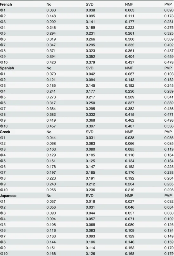
We propose Prototype Vector Projection (PVP), a dimensionality reduction method that uses a subset of the feature vectors as the basis vectors, and project all feature vectors spanned by these basis vectors. We refer to the set of basis vectors selected as theprototype vectors. Given a set ofnterms represented bym-dimensional feature vectors, PVP selects a subset ofd
<nvectors from this set as the prototype vectors. Pseudo code for PVP is shown inTable 1 Al-gorithm 1. First, we compute the centroid vector of the given set of feature vectors (Lines 2–4). Next, we rank the feature vectors by the number of non-zero elements that exist in the element-wise product between the centroid vector and each of the feature vectors. Elementelement-wise product between twom-dimensional vectors (x1,x2,. . .,xm)>and (y1,y2,. . .,ym)>is defined as them
-dimensional vector (x1y1,x2y2,. . .,xmym)>. As we show later in Proposition 1, the scores(x,c
(X)) indicates the likelihood that we would obtain dense vectors after the projection when we
use a feature vector as a prototype vector. Ideally, we would like to obtain dense vectors in the embedded space compared to that in the original space because, this would reduce the number of zero cosine similarity scores, thereby enabling us to measure similarity between terms more accurately. We select the feature vector with the maximum score as a prototype vector and re-move it from the current set of feature vectors. We repeat this process until we are left with ex-actlydnumber of prototype vectors. By removing the selected prototype vectors from the set of feature vectors that we use for computing the centroid in each iteration we increase the diversi-ty of the protodiversi-type vectors. Finally, we perform the Gram-Schmidt orthonormalization on the selected set of prototype vectors to create an orthonormal set of basis vectors [41]. Gram-Schmidt process produces a basis of orthonormal unit vectors from a given set of independent vectors. We project each feature vector to thed-dimensional space spanned by the prototype vectors by computing the inner-product of a feature vector with each of the prototype vectors. PVP is similar to random projection methods such as the locality sensitive hashing (LSH) [42,
Proposition 1.The average number of non-zero elements in the elementwise product between a prototype vectoryand a feature vectorxi2{x1,. . .,xn} is given by the number of non-zero
ele-ments in the elementwise product betweenyand the centroid vector of {x1,. . .,xn}.
Proof. Recall that the elements in the feature vectorsx1,. . .,xnare non-negative. Let us
de-fines(xi,y) as the number of non-zero elements in the elementwise product betweenxiandy. It
is given by,
sðxi;yÞ ¼ Xm
j¼1
Iðyjxij6¼0Þ:
Here,xijindicates thej-th dimension of the vectorxi. Then, the average number of non-zero
el-ements in the elementwise products betweenyand each of the feature vectors in {x1,. . .,xn} is
Table 1. Algorithm 1Prototype Vector Projection.
Input: A set ofnofmdimensional feature vectors {x1,. . .,xn}, the number of prototype vectorsd.
Output: The setf~x1;. . .;x~ngof projected vectors in thed-dimensional space.
1: Set of prototype vectorsP= {}
2:X= {x1,. . .,xn}
3:fori= 1toddo
4: Compute the centroid vectorc(X) of the set of vectors inXas follows cðXÞ ¼1
n X
x2X x
5: Compute the score,s(x,c(X)), for eachx2XbyPm
j¼1Iðxjcj6¼0Þ. Here,xjandcjare thej-th dimensions
ofxandc(X), and I is the indicator function defined as follows
IðyÞ ¼
(1 y¼True
0 otherwise
6: Select the vectorx*2Xwith the highest score. i.e.x¼argmax x2X
sðx;cðXÞÞ.
7: P=P[{x*} 8: X=X{x*}
9:end for
10: Perform Gram-Schmidt orthonormalization onPto obtain an orthonormal set of unit-length basis vectors {p1,. . .,pd}.
11:forxi2{x1,. . .,xn}do
12: ~xi¼ ½x>p1;. . .;x>pd
>
, Here,p1,. . .,pdare the prototype vectors computed and ordered following the
procedure in Lines 3–10. 13:end for
14:returnf~x1;. . .;x~ng
given by,
1
n Xn
i¼1
sðxi;yÞ ¼ 1 n
Xn
i¼1
Xm
j¼1
Iðyjxij6¼0Þ
¼ X
m
j¼1
I yj 1
n Xn
i¼1
xij
!
6¼0
!
¼ X
m
j¼1
Iðyj½cðx1;. . .;xnÞj6¼0Þ
¼ sðcðx1;. . .;xnÞ;yÞ:
Note that the summations over the instancesiand dimensionsjcan be inter-changed without affecting the number of non-zero element count because all elements in the feature vectors are non-negative. If this was not the case, we would have zero elements in the centroid because positive and a negative values can potentially cancel out during the computation of the centroid vector.
Several observations can be made about the above-mentioned dimensionality reduction process. First, the basis vectors used for the projection (i.e. prototype vectors) are selected from the given set of feature vectors. This is analogous to the cluster center selection process used in clustering algorithms such as thek-medoid clustering [44]. Unlikek-means clustering, where the cluster centers are not necessarily data points in the dataset, thek-medoid clustering algo-rithm always selects a data point from the given dataset closest to the centroid of the cluster. Compared to thek-means clustering, thek-medoid clustering algorithm is less prone to noise (outliers) because of its cluster center selection criterion.
Second, the feature values of the projected vectors are guaranteed to be non-negative be-cause we are considering the inner product between non-negative vectors (recall that character n-gram features are binary valued and contextual features are non-negative real values because we are using PPMI as the co-occurrence weighting measure). This property is particularly use-ful when we learn cross-lingual projections in the the next Section. Although there are other non-negative dimensionality reduction methods such as non-negative matrix factorization [27], they require optimizing a non-convex objective function, which is both computationally demanding as well as sensitive to the initial conditions. Note that dimensionality reduction methods such as singular value decomposition (SVD) or principal component analysis (PCA) do not necessarily produce negative projections even when the feature vectors are non-negative. On the other hand, PVP does not suffer from those drawbacks which makes it an ideal candidate for performing dimensionality reduction for learning a cross-lingual projection. Indeed as we show later, PVP outperforms SVD and NMF on a nearest neighbour prediction task using synthetic sparse data, and cross-lingual biomedical term translation prediction task using four real-world datasets for biomedical terms covering different target languages.
Learning Cross-Lingual Projections
Consider a pair of terms (wS,wT), wherewTis the translation ofwS. Let us denote the source
and target language feature vectors corresponding towSandwTrespectively by the boldfaced
fontswSandwT. Moreover, let us denote the lower-dimensional projections ofwSandwT
re-spectively bywS~ andwT~ . Note that the dimensionality ofwSandwTneed not be equal, and we
may select different numbers of features to represent terms in the source and the target lan-guages. Moreover, the number of prototype vectors selected in the PVP step need not be equal for the source and target languages. For example, we might decide to use 1000 prototype vec-tors from the source language feature vecvec-tors to project source language feature vecvec-tors to a 1000 dimensional space, whereas we might select 2000 prototype vectors from the target lan-guage feature vectors to project target lanlan-guage feature vectors to a 2000 dimensional space. Therefore, the dimensionalities ofwS~ andwT~ need not be equal. Given a set ofNtranslation pairsfðwSðiÞ;wT ðiÞÞgNi¼1, we learn a multivariate regression model,M, to predict the
corre-sponding target language feature vectorwT~ , given its source language feature vectorwS~ .
Exist-ing bilExist-ingual term lexicons or a manually annotated small seed translation term pairs can be used as the train data. We denote the predicted target language feature vector by the learnt multivariate regression modelMbyMðwS~ Þ. BecauseMdefines a mapping between the source
and the target language feature spaces, we call it across-lingual mappingin the remainder of this paper.
We use Partial Least Squares Regression (PLSR) [4] to learn a regression model using pairs of vectors. PLSR has been applied in Chemometrics [45], producing stable prediction models even when the number of samples is considerably smaller than the dimensionality of the fea-ture space. Given the rankrfor the regression space, PLSR attempts to project both source and the target language feature vectors to a commonrdimensional space such that the Pearson cor-relation coefficient between the two projected vectors is maximized in the lower dimensional space. The rankr, is often much smaller than the dimensionalities of the source or target lan-guage feature spaces and in practice set to values in the range [10, 100].
LetXandYdenote matrices formed by arranging respectively the vectorsw~ðSiÞs andw~
ðiÞ
T in
rows. PLSR decomposesXandYinto a series of products between rank 1 matrices as follows:
XX
r
l¼1
λlp>l ¼LP> ð2Þ
YX
r
l¼1
γlq>l ¼GQ>: ð3Þ
Here,λl,γl,pl, andqlare column vectors, and the summation is taken over the rank 1
matri-ces that result from the outer product of those vectors. The matrimatri-ces,Λ,Γ,P, andQare con-structed respectively by arrangingλl,γl,pl, andqlvectors as columns.
Pseudo code for learning a cross-lingual mapping,M, using PLSR is shown inTable 2 Algo-rithm 2. It is based on the two block NIPALS routine [46,47], and iteratively discoversLpairs of vectors (λl,γl) such that the covariances, Cov(λl,γl), are maximised under the constraint
jjpljj2=jjqljj2= 1. Finally, the mapping matrix,Mis computed usingλl,γl,pl,ql. The predicted
vectorM(wS) of a termwSin the source language to the target language is given by
Measuring Cross-Lingual Similarity
Once a cross-lingual mapping is learnt following the steps described in the previous section, we can use it to train a binary random forest classifier to detect translation pairs. Specifically, given a pair (wS,wT) of source and target terms that are in a translational relationship, we represent
this pair using a feature vector by concatenating the three vectors: (a)wS, source language
fea-ture vector of the source term, (b)wT, target language feature vector of the target term, and (c)
MwS, the projected source language feature vector using the learnt cross-lingual projection,M.
Let us denote the concatenated vector by [wS;wT;MwS]. Concatenated vectors from correct
translation pairs are labeled as positive training instances, whereas we randomly pair a source language term with a target language term to create an equal number of negative training in-stances. Next, we train a binary random forest model to classify the positive (translational pairs) and negative (non-translational pairs) instances. During test time, we use the class con-ditional probability returned by the trained random forest model that indicates how likely a given pair of terms belong to the positive class (i.e. correct translations). This probability is considered as the cross-lingual similarity between the source and the target terms. Finally, we rank target language terms in the descending order of the their cross-lingual similarities, and present the top-kterms as translation candidates forwSto the user. The user (e.g. a human
an-notator) can then select the best translation forwSfrom the returned ranked list instead of
going through a large list of possibly irrelevant terms.
There are several benefits of the above classification-based approach over directly measuring the similarity between a source term and a target term using their feature representations. First, the feature spaces in the source and target languages will not have much overlap, resulting in zero similarity scores.
Second, even if we use the learnt cross-lingual projection model,M, to first project the source language feature vectorwSand then measure the similarity betweenMwSandwTusing
some similarity measure such as the cosine similarity, we do not know which common features are salient for computing cross-lingual similarity. Different features might contribute
Table 2. Algorithm 2Learning a Cross-Lingual Mapping. Input:X,Y, Rankr.
Output: Mapping matrixM.
1: Randomly selectγlfrom columns inYl.
2:vl¼X
>
lγl=jjX
>
lγljj
3:λl=Xlvl
4:ql¼Y
>
lλl=jjY
>
lλljj
5:γl=Ylql
6: Ifγlis unchanged go to Line 7; otherwise go to Line 2
7:cl¼λ>lγl=jjλ
>
lγljj
8:pl¼X
>
lλl=λ
>
lλl
9:Xlþ1¼Xl λlp
>
l andYlþ1¼Yl clλlq
>
l.
10: Stop ifl=r; otherwisel=l+ 1 and return to Line 1. 11: LetC= diag(c1,. . .,cL), andV= [v1. . .vL]
12:M=V(P>V)−1C Q>
13:return M
differently to the similarity computation and we would like to learn some weight for each com-mon feature that indicates its importance for detecting cross-lingual similarity. The random forest binary classifier that we train will learn weights representing the discriminative capability of a feature for detecting correct translational term pairs from the incorrect ones.
Third, we might want to consider non-linear combinations of both source and target feature vectors for detecting correct translations. The random forest classifier generates a series of deci-sion trees (commonly known as a forest) that capture numerous combinations of features from both source and target feature vectors. Therefore, by using a random forest classifier instead a linear classifier, we can easily take into account the interaction between source language fea-tures and target language feafea-tures. Indeed, in our preliminary experiments using logistic regres-sion, a linear classification algorithm, resulted in poor performance, showing the importance of considering combinations of features from both source and target languages in order to ac-curately detect cross-lingual similarities.
Experiments
We conduct two types of experiments to evaluate the performance of the methods proposed in this paper. First, we evaluate the performance of the PVP method using synthetic data. Second, we evaluate the performance of the proposed cross-lingual similarity measure by using it to de-tect translations for English source biomedical terms in four target languages: French, Spanish, Greek, and Japanese.
Evaluating Prototype Vector Projection
The proposed PVP method computes a non-negative lower-dimensional embedding for a given set of feature vectors. Although the absolute similarity scores among vectors in the origi-nal (prior to embedding) and the embedded spaces can be different, if the relative ordering of similarity scores are preserved in the embedded space, we can consider such an embedding as desirable for finding nearest neighbors. We use this property to evaluate the performance of a dimensionality reduction method. To explain this idea concretely, let us consider four vectors
x,y1,y2, andy3in anm-dimensional space. Let us denote their projection to a lowerd(<m)
di-mensional space respectively by~x;y~1;y~2, andy~3. Let us assume that the similarity scores,
com-puted using some similarity measure such as cosine similarity, induce the following total ordering sim(x,y1)>sim(x,y2)>sim(x,y3). We can evaluate the accuracy of a dimensionality
reduction method by how well this original ordering of neighbors is preserved in the embedded space. Specifically, we can use the same similarity measure to compute the similarity scores
simðx~;~y1Þ,simðx~;~y2Þ, andsimðx~;y~3Þto create a total ordering of the neighbors with
respec-tive tox~, and compare the original ordering (i.e.y1y2y3) against the ordering of neighbors
with respect to~xafter the projection.
Two popular correlation coefficients that have been used for evaluation tasks in natural lan-guage processing [48,49] are the Pearson correlation coefficient (Pearson’sr), and the Kendall rank correlation coefficient (Kendall’sτ). Pearson’srcompares the absolute similarity scores between two vectors before and after the projection, whereas the Kendall’sτignores the abso-lute values of similarity and compares only the relative ranking of the neighbors before and after the projection. Therefore, by using bothrandτas evaluation measures, we can evaluate a dimensionality reduction method for its ability to preserve the topology of a vector space in the embedded space.
To define the evaluation measures we use, let us denote the similarity scores before and after the projection of the neighborsyiof a particular vectorxjrespectively by sim(xj,yi) and
defined by
rj¼
Pn 1
i¼1ðsimðxj;yiÞ mjÞðsimðx~j;~yiÞ m~jÞ
ffiffiffiffiffiffiffiffiffiffiffiffiffiffiffiffiffiffiffiffiffiffiffiffiffiffiffiffiffiffiffiffiffiffiffiffiffiffiffiffiffiffiffiffiffiffi Pn 1
i¼1 ðsimðxj;yiÞ mjÞ
2
q ffiffiffiffiffiffiffiffiffiffiffiffiffiffiffiffiffiffiffiffiffiffiffiffiffiffiffiffiffiffiffiffiffiffiffiffiffiffiffiffiffiffiffiffiffiffiffi Pn 1
i¼1 ðsimðx~j;~yiÞ m~jÞ
2
q ; ð5Þ
whereμjandm~jare the sample means of the the similarity scores respectively in the original
and the projected spaces. Specifically, they are given by,
mj ¼ 1
n 1
Xn
1
i¼1
simðxj;yiÞ;
~
mj ¼ 1
n 1
Xn
1
i¼1
simðx~j;~yiÞ:
Note that because there arenvectors in the dataset, the total number of neighbors for each vec-tor is the remainder of (n−1) vectors.
The Kendall’sτfor the same two groups of similarity scores are defined as follows
tj¼ 4Cðj;sjÞ
ðn 1Þðn 2Þ 1: ð6Þ
Here,ϕjandσjdenote the total orderings of indices of the neighbors ofxjrespectively in the
original and the embedded spaces, sorted in the descending order of their similarity scores with respect toxjandx~j, andC(ϕj,σj) is the number of concordant pairs between the two
permuta-tions. A pair of elements (p,q) is said to be concordant if the ranks assigned topandqin the two orderings do not contradict (i.e. ifpqin bothσandϕ, orpqin bothσandϕ).
We compute the Pearson’srand Kendall’sτcoefficients for the dataset consisting ofN in-stances as the average over the individual coefficients as follows
r ¼ 1
n Xn
j¼1
rj;
t ¼ 1
n Xn
j¼1
tj:
Both Pearson’srand Kendall’sτcoefficients are in the range [−1,1], where higher values
indi-cate positive correlations between the similarity scores (or relative rankings in the case of Ken-dall’sτ) in the original and the embedded spaces. Among different dimensionality reduction methods that project the same set ofndimensional vectors to the samedlower-dimensional space, we prefer methods that produce high Pearson’srand Kendall’sτvalues.
our feature vectors to zero with a 0.98 probability. Specifically, for each element in each feature vector we generate, we draw a random sample uniformly from the interval [0, 1], and set the corresponding element to zero if the drawn sample is less than 0.98. By following this process we obtain feature vectors that have on average 98% zeros. Following the same procedure, we create another dataset that has 1000 random vectors each with 10,000 dimensions. By using two synthetic datasets that have feature vectors of different dimensionalities we are able to veri-fy whether the trends observed depend on the dimensionality of the feature vectors.
We compare the Pearson and Kendall correlation coefficients obtained under varying di-mensionalities for the proposed prototype vector prediction (PVP) method against several di-mensionality reduction methods as described next.
L2. We select thedfeature vectors with the largest L2 norms as prototype vectors. The L2 norm of ann-dimensional vectorxis defined as
ffiffiffiffiffiffiffiffiffiffiffiffiffiffiffiffiffi Pn
j¼1xi2
q
. Recall that inTable 1 Al-gorithm 1, PVP selects prototype vectors based on the number of non-zero elements in feature vectors. An alternative approach would be to use L2 norm because if most of the elements in a vector are non-zero, it will result in a high L2 norm. However, this property does not always hold. For example, we might have feature vectors that contain only a handful of non-zero features but their absolute values might be large, resulting in high L2 norms. Nevertheless, feature vectors that are dense are likely to yield non-zero values when the cosine similarities are computed using them, which is useful when computing embeddings for the feature vectors. Note that L1 norm, given byPn
j¼1jxjj,
can also be used as a baseline method for selecting prototype vectors. However, both L1 and L2 norms induce the same total ordering among a given set of feature vectors. Therefore, we would obtain the same set of prototype vectors using both L1 and L2 norms. As a general result, it can be proved that any two normsjj jjαandjj jjβin a
fi-niteddimensional vector space are equivalent in the sense that there existm,M2R
such that for a vectorx2Rdthe inequalitiesmjjxjjα jjxjjβMjjxjjαhold [41].
There-fore, equivalent total orderings will be induced by different norms. We use L2 norm as a baseline method in our experiments to demonstrate the level of performance we would obtain if we simply use the vector norm for selecting prototype vectors.
SVD. Singular value decomposition (SVD) is a popular technique in NLP for performing di-mensionality reduction. It has been used in both attributional and relational similarity measurement tasks to overcome the sparseness of feature vectors, thereby reducing zero similarity scores [50]. Given a matrixA(not necessarily a square matrix), SVD de-composesAinto the product of three matricesU,D, andVgiven by
A¼UDV>;
whereUandVare in column orthonormal form (i.e.U>U=V>V=I), andDis a di-agonal matrix containing the singular values ofAas the diagonal elements [41]. The rank ofDis equal to that ofA. For an integerdlesser than the rank ofA, the matrix
^
A¼UdDdV>
d gives thed-dimensional approximation toAin the sense that the
Fro-benius norm of the approximation error,jjA A^ j jFis minimized byA^ ¼
UdDdV>
d among all matrices with rankd. Here,UdandVdare created by selecting
respectively the left and right singular vectors ofUandVcorresponding to the largest singular values ofA[40]. However, the elements inAdare not necessarily non-negative
cosine similarity scores giving rise to negative similarity scores. In practice, approxi-mately half of the elements inAdare negative. Turney [51] proposed a solution to this
problem by setting the negative values inAdto zero. We implement this method as a
baseline for comparison.
NMF. Given a matrixA2Rn×mthat contains non-negative elements, non-negative matrix
factorization (NMF) [27,52,53] decomposesAinto the product of two non-negative matricesW2Rn×kandH2Rk×msuch that,
A¼WH:
In particular, the matrixWcan be seen as a lowerk-dimensional representation of the givennvectors. We use the rows in matrixWcomputed using projected gradient-based NMF algorithm implemented in scikit-learn library (http://scikit-learn.org/) as a baseline dimensionality reduction method for comparisons.
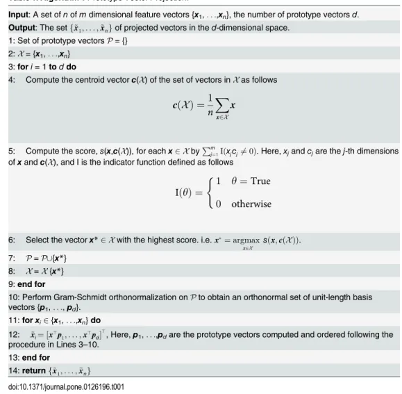
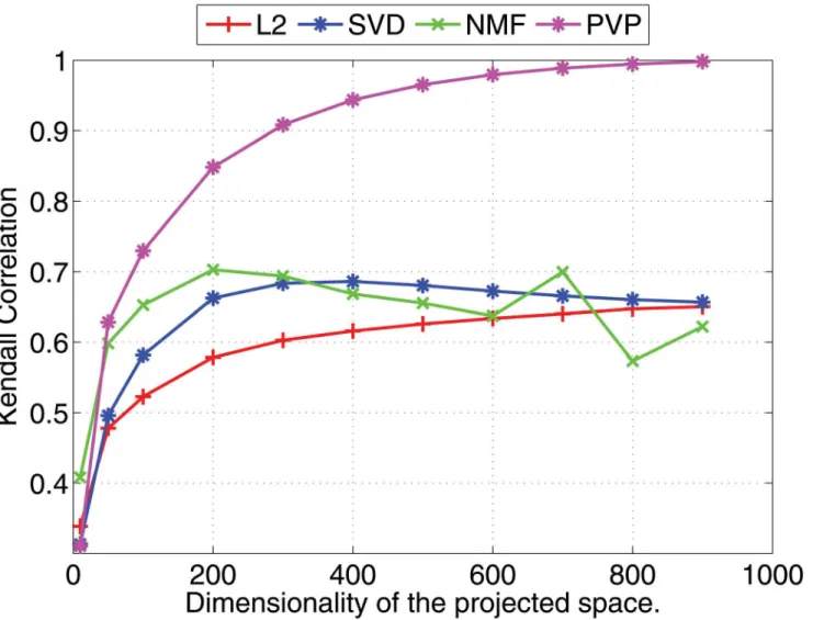
Experimental results are shown in Figs1and2(for 1000 dimensional feature vectors) and Figs3and4(for 10,000 dimensional feature vectors). As an overall trend in both Figures, we see that all methods are performing equally when the dimensionality of the projected space is very small. However, the correlation coefficients for such low dimensional projections are also very low because most of the important features of the original space are lost as a result of the aggressive lower dimensional projections. When we increase the dimensionality both Pearson and Kendall correlation coefficients improve. However,SVDandNMFmethods quickly saturates to almost fixed correlations and by further increasing the dimensionality we cannot improve their performance. On the other hand, the correlation coefficients withPVP continu-ously increase. BecauseSVDandNMFare computing low rank approximations to the matrix defined by the feature vectors, the correlation does not improve when we have reached the rank of the data matrix. Moreover, minimization of the Frobenius norm of the approximation as done bySVDdoes not guarantee a high correlation between similarity scores computed using the lower dimensional projections of the feature vectors. In the larger 10,000 dimensional setting depicted in Figs3and4, we see that Kendall’sτdrops forSVDandNMFmethods when the dimensionality is increased beyond 300 dimensions. In practice, it is difficult to determine the optimal value of the dimensionality for the projection. Therefore, in practice projection methods that do not loose performance due to extra dimensions are desirable. Per-formance of theL2baseline varies and is not robust. For example, in the 10,000 dimensional case (Fig 3),L2method reports the worst Pearson correlation among the four methods compared.
Overall, the projected feature vectors usingNMFare almost 100% dense, whereasSVDwith negative values set to zero produces ca. 50% dense vectors. Vectors projected byPVPare ca. 60% dense, giving an intermediate level of density compared toNMFandSVD. In particular, considering that the original feature vectors were only 2% dense (i.e. 98% sparse), all three methods can be seen as producing dense vectors in the lower-dimensional space. Although we do not explore data visualization in this paper, the different densities produced by these meth-ods could be of interest to lower-dimensional data visualization tasks [54].
In addition to the experiments described above which use artificial data, we also conduct a second experiment using the monolingual feature vectors we created for the English source lan-guage. We use 1000 dimensional contextual feature vectors for 2454 English source terms, and apply the dimensionality reduction methods described in the previous paragraph. We compare the nearest neighbors in the original feature space to that in the projected feature space using Kendall rank correlation coefficient and the Pearson’s correlation coefficient as shown in Figs5
be observed in Figs5and6, and the difference between PVP and other methods is more significant.
Evaluating Cross-Lingual Similarity Measurement
Cross-Lingual Biomedical Terms Dataset. To evaluate the proposed cross-lingual simi-larity measure, we apply it in a biomedical term translation detection task. We use the dataset created by Kontonatsios et al. [24], which lists translations for English biomedical terms in four target languages: French, Spanish, Greek, and Japanese. Next, we briefly describe the process followed by Kontonatsios et al. [24] to construct this dataset. First, 4000 English Wikipedia ar-ticles are selected covering 4000 English biomedical terms. Second, Wikipedia interlingual links are used to retrieve thematically related articles in each of the target languages. However, not all of the 4000 English articles are translated into all the target languages. Therefore, differ-ent lists of query-terms were used to retrieve Wikipedia articles for differdiffer-ent language pairs. For training purposes, we used 5,000 pairs of source and target language terms for each
Fig 1. Nearest neighbor prediction with artificial data.Pearson’srcorrelation coefficients for different dimensionality reduction methods are shown under varying dimensionalities (Feature vectors are 1000 dimensional).
language pair, whereas, for testing additional 1000 source terms were used. Train and test term pairs are manually selected from UMLS.
Evaluation Measure. We compute precision@R for different levels of rank R. Precision@R is defined as
Precision@R¼total number of correct translations among top R ranked candidates
R :ð7Þ
We compute Precision@R values for each test case in our test dataset and compute the average of those values as the evaluation measure. Precision@R is a standard evaluation measure in in-formation retrieval [55], where the search results ranked and returned by an information re-trieval system is evaluated for its precision at different ranks. An information rere-trieval system that ranks relevant results among the top ranked candidates is desirable, and Precision@R mea-sure captures this notion.
Fig 2. Nearest neighbor prediction with artificial data.Kendall’sτ(right) correlation coefficients for different dimensionality reduction methods are shown under varying dimensionalities (Feature vectors are 1000 dimensional).
Results. We use Precision@R values to evaluate character n-gram features and contextual features as used in the proposed method. We compare the proposedPVP-based dimensionality reduction method againstSVDandNMFmethods, which were defined under the experiments conducted using synthetic data. Specifically, inPVP,SVD, andNMFmethods, we represent a term pair (wS,wT) using the concatenated vector½wS~ ; ~wT;MwS~ when training the random
forest classifier. TheNobaseline denotes the level of performance we would obtain if we had not use any dimensionality reduction methods, but had used the original feature spaces to train the random forest binary classifier. Specifically, inNobaseline, we represent a term pair (wS,
wT) using the concatenated vector [wS;wT;MwS] when training the random forest classifier,
Any differences in thefinal performance betweenNoand each of theSVD,NMF, andPVP
methods can be directly attributable to the learnt cross-lingual projection modelMusing each dimensionality reduction method.
We use 10,000 dimensional feature vectors for source and target term representations with both character n-grams as well as contextual features. Prior work studying cross-lingual
Fig 3. Nearest neighbor prediction with artificial data.Pearson’srcorrelation coefficients for different dimensionality reduction methods are shown under varying dimensionalities (Feature vectors are 10000 dimensional).
biomedical term translations has reported that 10,000 features are sufficient to obtain high-quality translation candidates [23]. The proposed PVP method was used to project these 10,000 dimensional feature space to 2,000 dimensions. We learn the PLSR model inTable 2 Al-gorithm 2 with 10 components. Random forest classifier is trained with 150 trees. BothSVD
andNMFmethods are used with 2,000 dimensions, the exact same number of dimensions as used byPVP. Therefore, any differences amongPVP,SVD, andNMFmethods can be consid-ered as resulting from their dimensionality reduction method instead of the dimensions.
For each target language, we denote the level of performance for ranks 1–10. In each test case, we have one or two correct target language translations listed for each source language term. In order to obtain non-zero Precision@R values, a method must rank those correct trans-lations among the top 10 ranked candidates from a pool of 1000 target language terms. We consider this strict evaluation criteria not only enables us to differentiate the performance of the different methods we compare, but also resembles the perceived application of the
Fig 4. Nearest neighbor prediction with artificial data.Kendall’sτ(right) correlation coefficients for different dimensionality reduction methods are shown under varying dimensionalities (Feature vectors are 10000 dimensional).
proposed method—suggesting target language translation candidates for a given source lan-guage biomedical term to support the manual annotation process of biomedical
bilingual dictionaries.
FromTable 3we see that for French, Greek, and Japanese languages there is a clear benefit of using the projected features produced by the proposedPVP. However, the performance de-creases when projected features are used for Spanish. For all four target languages,PVP consis-tently outperformsSVDandNMF, demonstrating its accuracy as a dimensionality
reduction method.
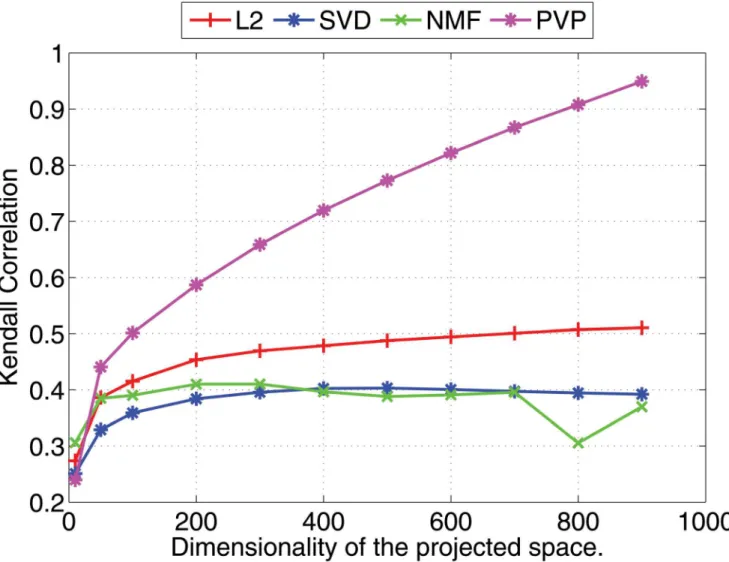
In the case of contextual features shown inTable 4, we see thatPVPreports the best results for all rank levels for French and Spanish. For Greek and Japanese,PVPreports better results when we consider all rank values except at the first rank. Nevertheless,PVPconsistently out-performSVDandNMFfor all target languages and all ranks when we use contextual features, as it did with the character n-gram features. The ability of the proposedPVPmethod to work well with different types of features is important because it enables us to experiment with
Fig 5. Nearest neighbor prediction with English feature vectors.Pearson’srcorrelation coefficients for different dimensionality reduction methods are shown under varying dimensionalities (Feature vectors are 1000 dimensional).
numerous feature types. Overall, compared to character n-gram feature-based results shown in
Table 3, the Precision@R values obtained using contextual features shown inTable 4are low. Compared to the character n-gram features, the distribution of the context features is dispersed because of the large number of unigrams and bigrams extracted as contextual features. There-fore, contextual feature vectors are high dimensional and sparse compared to character n-gram feature vectors. Moreover, contextual features are extracted from the local context of the terms and might not necessarily be strongly related to the term under consideration. Therefore, the association measure we use to evaluate the strength of the relationship between a term and its contextual features becomes important. On the other hand, character n-gram features are ex-tracted directly from the term itself, and does not require any weighting.
A particularly interesting observation from our analysis is the high precision scores obtained using the character n-gram feature projection in the English-Japanese translation task. These two languages use different alphabets. Therefore, the character n-gram feature spaces between English and Japanese do not overlap. Despite this difficulty, we can learn a cross-lingual
Fig 6. Nearest neighbor prediction with English feature vectors.Kendall’sτ(right) correlation coefficients for different dimensionality reduction methods are shown under varying dimensionalities (Feature vectors are 1000 dimensional).
Table 3. Precision@rank values for English as the source language and different target languages using character n-gram features.
French No SVD NMF PVP
@1 0.263 0.121 0.091 0.297
@2 0.369 0.194 0.163 0.415
@3 0.439 0.254 0.238 0.494
@4 0.506 0.337 0.289 0.539
@5 0.543 0.377 0.345 0.574
@6 0.564 0.415 0.381 0.597
@7 0.590 0.458 0.411 0.615
@8 0.614 0.501 0.470 0.624
@9 0.636 0.536 0.509 0.640
@10 0.647 0.556 0.546 0.653
Spanish No SVD NMF PVP
@1 0.145 0.086 0.112 0.130
@2 0.243 0.150 0.166 0.200
@3 0.304 0.215 0.228 0.261
@4 0.358 0.270 0.263 0.324
@5 0.401 0.319 0.322 0.385
@6 0.443 0.361 0.370 0.420
@7 0.478 0.401 0.412 0.457
@8 0.508 0.435 0.449 0.492
@9 0.549 0.490 0.476 0.521
@10 0.576 0.532 0.517 0.543
Greek No SVD NMF PVP
@1 0.07 0.089 0.101 0.224
@2 0.099 0.170 0.166 0.305
@3 0.136 0.235 0.224 0.351
@4 0.172 0.284 0.284 0.375
@5 0.191 0.331 0.333 0.390
@6 0.211 0.369 0.383 0.403
@7 0.242 0.420 0.426 0.409
@8 0.256 0.456 0.458 0.418
@9 0.274 0.490 0.491 0.426
@10 0.296 0.529 0.528 0.431
Japanese No SVD NMF PVP
@1 0.048 0.041 0.018 0.162
@2 0.066 0.075 0.043 0.193
@3 0.097 0.094 0.060 0.223
@4 0.127 0.115 0.086 0.250
@5 0.142 0.143 0.103 0.261
@6 0.164 0.153 0.126 0.274
@7 0.179 0.168 0.140 0.287
@8 0.204 0.191 0.168 0.297
@9 0.218 0.210 0.191 0.303
@10 0.232 0.224 0.208 0.314
Table 4. Precision@rank values for English as the source language and different target languages using contextual features.
French No SVD NMF PVP
@1 0.083 0.038 0.063 0.090
@2 0.148 0.095 0.111 0.173
@3 0.202 0.141 0.177 0.231
@4 0.248 0.189 0.223 0.275
@5 0.294 0.231 0.261 0.325
@6 0.319 0.266 0.300 0.369
@7 0.347 0.295 0.332 0.402
@8 0.371 0.323 0.361 0.437
@9 0.394 0.352 0.404 0.459
@10 0.420 0.379 0.437 0.478
Spanish No SVD NMF PVP
@1 0.070 0.042 0.087 0.103
@2 0.121 0.094 0.143 0.182
@3 0.185 0.145 0.192 0.245
@4 0.241 0.177 0.230 0.289
@5 0.273 0.217 0.289 0.341
@6 0.317 0.250 0.337 0.389
@7 0.354 0.295 0.382 0.436
@8 0.382 0.332 0.415 0.471
@9 0.419 0.368 0.462 0.498
@10 0.457 0.397 0.487 0.536
Greek No SVD NMF PVP
@1 0.044 0.031 0.038 0.036
@2 0.068 0.063 0.066 0.085
@3 0.103 0.080 0.085 0.119
@4 0.129 0.105 0.110 0.164
@5 0.151 0.125 0.134 0.184
@6 0.178 0.147 0.152 0.225
@7 0.197 0.165 0.170 0.238
@8 0.223 0.191 0.192 0.264
@9 0.240 0.212 0.204 0.285
@10 0.256 0.236 0.219 0.298
Japanese No SVD NMF PVP
@1 0.037 0.018 0.027 0.032
@2 0.056 0.031 0.046 0.064
@3 0.090 0.044 0.057 0.080
@4 0.094 0.057 0.071 0.102
@5 0.108 0.068 0.080 0.126
@6 0.116 0.083 0.109 0.134
@7 0.133 0.093 0.129 0.149
@8 0.144 0.106 0.140 0.159
@9 0.151 0.114 0.153 0.170
@10 0.168 0.126 0.168 0.179
projection model between the character n-gram feature spaces between English and Japanese that can be used to correctly identify translations. Character n-gram models have been reported to be sensitive to the distance between languages in prior work on term translation [24].
The dimensionality reduction conducted by PVP can be seen as projecting similar features in each language to the same dimension in the lower-dimensional space. On the other hand, the random forest classifier can be seen as considering the interactions between the dimensions in the source and target language lower-dimensional spaces created by PVP. The cross-lingual projection further improves the cross-lingual similarity measurement by reducing the mis-match between source and target feature spaces.
Discussion and Conclusions
We considered the problem of measuring the similarity between technical terms such as bio-medical terms across different languages. For this purpose, we proposed a cross-lingual similar-ity measure by first representing source and target language terms using character n-gram features or contextual features. We then project feature vectors in each language to a lower-di-mensional space to reduce the number of features used in the representations. We proposed PVP for this purpose. PVP selects a subset of the feature vectors as prototype vectors and use those as basis vector to project the given set of feature vectors to a lower dimensional space.
Next, we proposed a method to learn a cross-lingual projection model using the partial least squares regression (PLSR). Finally, we trained a binary random forest classifier to discriminate positive (translational pairs) vs. negative (non-translational pairs), and use the class conditional probability returned by the trained random forest classifier as a cross-lingual similarity mea-sure to rank the target language translational candidates for a given source language term.
We compared the proposed PVP method against previously proposed dimensionality re-duction methods such as the singular value decomposition (SVD), and non-negative matrix factorization (NMF), as well as a baseline method that uses the L2 norm of the feature vectors to select the prototype vectors. Our experimental results on two synthetic datasets show the su-periority of the proposed PVP method for dimensionality reduction. We apply the proposed cross-lingual similarity measure to find translations for English source terms in four target lan-guages: French, Spanish, Greek, and Japanese. Our experimental results show that except for Spanish, for all other languages we can improve the performance of the translation detection by projecting character n-gram features.
Several interesting future research directions of the current work can be identified. Given that character n-gram features and contextual features capture different properties of terms (i.e. intrinsic vs. extrinsic), an obvious next step would be to combine those feature spaces to better represent a pair of terms. We note that the main contributions of our work, PVP and cross-lingual projection learning, are independent of any feature spaces that we use to repre-sent terms in the source and the target languages. Therefore, in principle our proposed meth-ods can be used with different feature spaces. Improving cross-lingual similarity measurement using different features is a complementary research direction beyond the scope of this paper. Nevertheless we mention that there are several important challenges that one must overcome when combining different feature spaces such as weighting and normalizing different groups of features in a consistent manner. For example, character n-gram features are binary whereas PPMI-weighted contextual features are real-valued. How to combine these two types of fea-tures and whether we should normalize feature vectors prior to training, if so using which norm, are all important design decisions.
has three constituent words might appear only a small number of times even in a large corpus, which makes it difficult to extract sufficiently larger number of contextual features to represent the term. This leads to sparse contextual feature vectors, which becomes problematic during cross-lingual similarity measurement. On the other hand, the individual words in the term might be more popular and are likely to have many contextual features. Therefore, if we can compute the representation for the term using the representations for the individual words in the term, we can obtain a dense representation for the term.
Several variants of the PVP algorithm presented inTable 1Algorithm 1 are possible de-pending the structure of the data. For example, if the dataset that we would like to perform di-mensionality reduction on consists of multiple clusters, then we could first apply a clustering algorithm such as k-means to produce the inherent clusters in the dataset. Next, we can select a set of prototypes considering each cluster separately to select a representative set of prototype vectors that could be used for the dimensionality reduction step.
The prototype selection criterion of PVP can also be replaced with other criteria. For exam-ple, we could select prototype vectors not only by their ability to produce dense vectors in the projected space but also to maximize the diversity of the selected set of prototype vectors. PVP algorithm presented inTable 1Algorithm 1 selects prototype vectors based on the number of non-zero elements in them, and attempts to reduce the redundancy in the prototype vectors by iteratively removing the prototype vectors selected at each round. Alternatively, we could select prototype vectors that simultaneously maximizes an objective function consisting of two fac-tors: (a) average number of non-zero elements in the set of prototype vectors selected so far, and (b) the average pairwise dissimilarity between all pairs of prototype vectors selected so far.
In our future work, we plan to explore these research directions.
Supporting Information
S1 dataset. We publicly release the processed feature vectors used by the proposed method to facilitate future comparisons.
(TGZ)
Author Contributions
Conceived and designed the experiments: DB. Performed the experiments: DB. Analyzed the data: DB. Contributed reagents/materials/analysis tools: DB GK SA. Wrote the paper: DB.
References
1. Dagan I, Church K (1994) Termight: Identifying and translating technical terminology. In: Proc. of the fourth conference on Applied Natural Language Processing. pp. 34–40.
2. Och FJ, Ney H (2003) A systematic comparison of various statistical alignment models. Computational Linguistics 29: 19–51. doi:10.1162/089120103321337421
3. Vuli I, Moens MF (2014) Probabilistic models of cross-lingual semantic similarity in context based on la-tent cross-lingual concepts induced from comparable data. In: Proc. of Empirical Methods in Natural Language Processing (EMNLP). pp. 349–362.
4. Wold H (1985) Partial least squares. In: Kotz S, Johnson NL, editors, Encyclopedia of the Statistical Sciences, Wiley. pp. 581–591.
5. Breiman L (2001) Random forests. Machine Learning 45: 5–32. doi:10.1023/A:1010933404324
6. Bollegala D, Matsuo Y, Ishizuka M (2007) An integrated approach to measuring semantic similarity be-tween words using information available on the web. In: Proceedings of NAACL HLT. pp. 340–347. 7. Yokote K, Bollegala D, Ishizuka M (2012) Similarity is not entailment—jointly learning similarity