Towards adaptable, interactive and quantitative paleogeographic maps

(1)

BGD

9, 9603–9636, 2012

Interactive paleogeographic

maps

N. Wright et al.

Title Page

Abstract Introduction

Conclusions References

Tables Figures

◭ ◮

Back Close

Full Screen / Esc

Printer-friendly Version Interactive Discussion

Discussion

P

a

per

|

Dis

cussion

P

a

per

|

Discussion

P

a

per

|

Discussio

n

P

a

per

|

Biogeosciences Discuss., 9, 9603–9636, 2012 www.biogeosciences-discuss.net/9/9603/2012/ doi:10.5194/bgd-9-9603-2012

Biogeosciences Discussions

This discussion paper is/has been under review for the journal Biogeosciences (BG). Please refer to the corresponding final paper in BG if available.

Towards adaptable, interactive and

quantitative paleogeographic maps

N. Wright, S. Zahirovic, R. D. M ¨uller, and M. Seton

EarthByte Group, School of Geosciences, The University of Sydney, Sydney, NSW 2006, Australia

Received: 12 July 2012 – Accepted: 16 July 2012 – Published: 31 July 2012

Correspondence to: N. Wright (nwri5277@uni.sydney.edu.au) and S. Zahirovic (sabin.zahirovic@sydney.edu.au)

(2)

BGD

9, 9603–9636, 2012

maps

N. Wright et al.

Title Page

Tables Figures

◭ ◮

Back Close

Full Screen / Esc

Discussion

P

a

per

|

Dis

cussion

P

a

per

|

Discussion

P

a

per

|

Discussio

n

P

a

per

|

Abstract

A variety of paleogeographic atlases have been constructed, with applications from pa-leoclimate, ocean circulation and faunal radiation models to resource exploration; yet their uncertainties remain difficult to assess, as they are generally presented as low-resolution static maps. We present a methodology for ground-truthing paleogeographic

5

maps, by linking the GPlates plate reconstruction tool to the global Paleobiology Database and a Phanerozoic plate motion model. We develop a spatio-temporal data mining workflow to compare a Phanerozoic Paleogeographic Atlas of Australia with bio-geographic indicators. The agreement between fossil data and paleobio-geographic maps is quite good, but the methodology also highlights key inconsistencies. The Early

De-10

vonian paleogeography of southeastern Australia insu_fficiently describes the Emsian inundation that is supported by biogeography. Additionally, the Cretaceous inundation of eastern Australia retreats by 110 Ma according to the paleogeography, but the bio-geography indicates that inundation prevailed until at least 100 Ma. Paleobiobio-geography can also be used to refine Gondwana breakup and the extent of pre-breakup Greater

15

India can be inferred from the southward limit of inundation along western Australia. Although paleobiology data provide constraints only for paleoenvironments with high preservation potential of organisms, our approach enables the use of additional proxy data to generate improved paleogeographic reconstructions.

1 Introduction

20

The geography of continents has varied considerably through time, driven by plate tec-tonic processes, crustal thickening and thinning, erosion, sedimentation, and global and regional sea level fluctuations (Miller et al., 2005; M ¨uller et al., 2008), driving both biological radiations and occasional mass extinctions (Hallam and Cohen, 1989; Hal-lam and Wignall, 1999; Stanley, 1988). In particular, the Mesozoic amalgamation and

25

(3)

BGD

9, 9603–9636, 2012

maps

N. Wright et al.

Title Page

Tables Figures

◭ ◮

Back Close

Full Screen / Esc

Discussion

P

a

per

|

Dis

cussion

P

a

per

|

Discussion

P

a

per

|

Discussio

n

P

a

per

|

the paleogeographic, paleobiological, tectonic and climatic evolution of the planet as it resulted in the opening and closure of oceanic gateways that regulated and impacted climate patterns (Cocks and Torsvik, 2002; Scotese et al., 1999; Torsvik and van der Voo, 2002; Golonka et al., 2006; Seton et al., 2012). The ability to create interactive digital models of paleogeography enables the estimation of land and ocean

distribu-5

tions that can be linked to paleo-climate simulations as demonstrated by Gyllenhaal et al. (1991), Ross et al. (1992), Donnadieu et al. (2006) and others. A variety of global and regional paleogeographic atlases have been constructed, but their di_fferences and uncertainties are difficult to assess. Conventional paleogeographic reconstructions are static maps, often with poor temporal and spatial resolutions and usually tied to one

10

plate motion model. Such models tend to fall short in documenting the wide range of source data and reasoning for their interpretations, i.e. the “decision tree” that led to a given set of published maps is usually unknown, including the interpretative weighting of di_fferent data types leading to a given interpretation of facies boundaries, paleocoast-lines or outpaleocoast-lines of mountain belts. Traditional paleogeographic maps are superimposed

15

on specific plate tectonic reconstructions based on paleomagnetic data, faunal data (Cocks and Torsvik, 2002) or reinterpretations of existing paleogeographic reconstruc-tions (Ford and Golonka, 2003; Golonka, 2007). However such maps quickly become outdated as plate motion models are refined and proxy data is improved. Paleogeo-graphic maps are published infrequently and are typically difficult to replicate, modify

20

and use to constrain the evolution of regional basins with numerical simulations. Using the GPlates plate-reconstruction tool, we link the paleobiological data to a global plate motion model that spans the entire Phanerozoic. We focus on Australia to test our methodology, because a regional paleogeographic atlas for Australia is pub-licly available in digital vector graphics form (Langford et al., 2001), spanning the last

25

(4)

BGD

9, 9603–9636, 2012

maps

N. Wright et al.

Title Page

Tables Figures

◭ ◮

Back Close

Full Screen / Esc

Discussion

P

a

per

|

Dis

cussion

P

a

per

|

Discussion

P

a

per

|

Discussio

n

P

a

per

|

development in the field. There are 70 time slices that cover the entire Phanerozoic, with interpretations largely based on lithological indicators of paleoenvironments (Ta-ble 1), structural and tectonic histories and other geological arguments from outcrops and well data. The complete temporal coverage of the Phanerozoic results in a consis-tent approach to interpreting the changing environments of the entire Australian

conti-5

nent, while the digital provision of input data and subsequent interpretations make this paleogeographic model testable and expandable. To complement the paleogeographic model, we use biogeographic indicators embedded in the open-source community Pa-leobiology Database that contains entries for almost 130 000 fossil collections and over one million individual fossil occurrences with global coverage. It is a growing resource

10

that is regularly updated, meaning that paleogeographic models can be made to be adaptable rather than presented as static maps.

We integrate the paleogeographic model with a Phanerozoic plate reconstruction model using GPlates in order to uncover spatio-temporal correlations and test the fi-delity of the existing paleogeographic model in the context of biogeographic indicators

15

from paleobiology. Our paleogeographic reconstructions can be easily linked to alter-native plate motion models, have flexible spatial and temporal resolutions, and can be updated interactively. Our paleogeographic interpretations are testable and replica-ble as the paleogeography model and paleobiology data are made availareplica-ble in digital form in the Supplement. We use a data mining approach to expose the relationships

20

(5)

BGD

9, 9603–9636, 2012

maps

N. Wright et al.

Title Page

Tables Figures

◭ ◮

Back Close

Full Screen / Esc

Discussion

P

a

per

|

Dis

cussion

P

a

per

|

Discussion

P

a

per

|

Discussio

n

P

a

per

|

2 Methods

2.1 Phanerozoic plate reconstructions

We base our Phanerozoic relative plate motions on the rotation model made available in the supplementary section of Golonka (2007), and use block outlines based on ter-rane boundaries used in Seton et al. (2012) and interpretations of magnetic and

grav-5

ity anomalies. Paleozoic plate motions are based on continental paleomagnetic data due to the absence of preserved seafloor spreading histories. Although paleomagnetic data on continents do not provide paleo-longitudes, the relative plate motions can be inferred from commonalities in the apparent-polar wander (APW) paths (van der Voo, 1990). If two or more continents share a similar APW path for a time period, then it can

10

be inferred that these continents were joined for these times. In the ideal world such APW paths would coincide perfectly, but due to the inherent uncertainties and errors in paleomagnetic measurements, we assume that the clustering of paleo-poles indi-cates a common tectonic history between two or more plates during Paleozoic times. Similarly, tectonic affinities can be deduced from the continuity of orogenic belts,

sed-15

imentary basins, volcanic provinces, biogeographic indicators and other large-scale features across presently-isolated continents (Wegener, 1915).

We assign motions to Africa, as the base of our rotation hierarchy, for the Phanero-zoic based on the smoothed APW spline path from Torsvik and van der Voo (2002). All continents that moved independently in the absolute reference frame (i.e. relative to

20

the spin axis) from the Golonka (2007) model were recalculated as equivalent relative rotations to a conjugate neighbouring plate, connected hierarchically in our plate circuit as described in Fig. 1. The paleobiogeography is used to test the plate motion histo-ries, and more specifically the evolution of the rift zones resulting from initial Gondwana breakup.

(6)

BGD

9, 9603–9636, 2012

maps

N. Wright et al.

Title Page

Tables Figures

◭ ◮

Back Close

Full Screen / Esc

Discussion

P

a

per

|

Dis

cussion

P

a

per

|

Discussion

P

a

per

|

Discussio

n

P

a

per

|

2.2 Paleobiology database

The Paleobiology Database (http://paleodb.org) is a compilation of global taxonomic data covering deep geologic time. Fossil collections were downloaded in four groups on 6 October 2011: general (43 878), carbonate marine (34 542), siliciclastic marine (21 576) and terrestrial (22 385). Metadata for each fossil collection were preserved;

5

including the source, present-day co-ordinate, temporal range, lithology of host rock, paleoenvironment, taxonomic descriptors, the collection method and many others (see Supplement). Only collections with temporal and paleoenvironmental assignments were included, with a total of 122 381 fossil collections. Fossil data were assigned GPML (GPlates Mark-up Language) attributes such as appearance and

disappear-10

ance ages based on the fossil collection’s temporal range (Fig. 2). Assemblages were assigned Plate IDs based on their location within present day continental polygons in order to reconstruct the past positions of the fossil collections.

2.3 Data mining

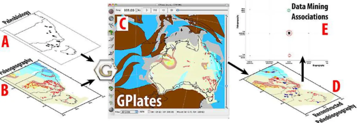
The paleogeography and biogeography of Australia was embedded within the global

15

Phanerozoic plate reconstructions. Fossil collections and the Australian paleogeog-raphy were reconstructed in GPlates at 1 Myr intervals and were used as the seed dataset for extracting the paleogeography (Fig. 3). The spatio-temporal associations between the paleogeography and biogeography through time were analysed to high-light inconsistencies with the aim of improving the paleogeographic model.

Inconsis-20

tencies between the paleogeographic maps and biogeographic indicators were high-lighted for the Emsian paleogeography of southeastern Australia using workflows in the statistical analysis package Orange (see Supplement). The raw fossil collection data was assumed to be a true representation of the paleoenvironment at the recon-structed time, while the paleogeography is an interpretation of other raw data,

includ-25

(7)

BGD

9, 9603–9636, 2012

maps

N. Wright et al.

Title Page

Tables Figures

◭ ◮

Back Close

Full Screen / Esc

Discussion

P

a

per

|

Dis

cussion

P

a

per

|

Discussion

P

a

per

|

Discussio

n

P

a

per

|

marine environment were treated as inconsistencies requiring refinement of the paleo-geographic model.

3 Results

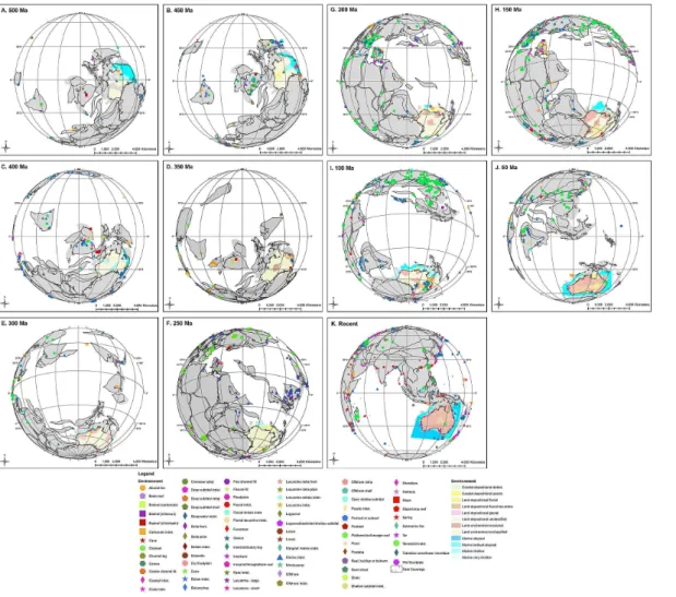
The linked plate tectonic, paleogeographic and biogeographic reconstructions are pre-sented for the Phanerozoic in 50 Myr intervals (Fig. 4). By the end Cambrian, Australia

5

was part of the eastern Gondwana megacontinent and spanning equatorial latitudes. The easternmost Australian continent developed in the Paleozoic, marked by the Tas-man Line that separates the western cratonic portion of the continent from the younger lithosphere to the east. The northern margin of Gondwana was composed of the east Asian terranes, including North China, South China, Tarim, Tibet, Indochina and the

10

Cimmerian super-terrane. These terranes consecutively detached, to open and subse-quently consume the Tethyan oceans, and amalgamated in the northern hemisphere to form the Eurasian continent (Metcalfe, 1994). The breakup of Pangea continued with the dispersal of Gondwana continents, with India and Australia detaching from Antarc-tica in the Cretaceous in a generally northward trajectory (Fig. 4).

15

3.1 500 Ma (Cambrian)

During the earliest Phanerozoic, Australia is located at equatorial latitudes. Fossil data are sparse globally in the Cambrian and the Paleogeographic Atlas of Australia (Lang-ford et al., 2001) is incomplete during this time. The eastern shelf of Australia is an abyssal environment at this time (Fig. 4a), with an east-west band of shallow marine

20

(8)

BGD

9, 9603–9636, 2012

maps

N. Wright et al.

Title Page

Tables Figures

◭ ◮

Back Close

Full Screen / Esc

Discussion

P

a

per

|

Dis

cussion

P

a

per

|

Discussion

P

a

per

|

Discussio

n

P

a

per

|

3.2 450 Ma (Ordovician – Silurian)

Global fossil data predominantly indicate marine environments in the Ordovican and Silurian. Based on the Paleogeographic Atlas of Australia, a bathyal-abyssal environ-ment is present along eastern Australia, whilst shallow marine and coastal depositional environments are distributed in an east-west band across the continent (Langford et

5

al., 2001). Available paleobiology data correlate well with Australian paleogeography reconstructions, indicating a marine environment in eastern Australia based on the presence of basinal (siliciclastic), carbonate indeterminate, and deep subtidal biogeo-graphic data at 450 Ma (Fig. 4b).

3.3 400 Ma (Devonian)

10

Inundation of the present day Australian continent has reduced, with the eastern shelf of Australia classified as a bathyal-abyssal environment and an area of shallow marine towards the central portion of the continent (Fig. 4c). Paleobiology indicators correlate well with the paleogeographic data; fossil data implies a marine environment along the present day east coast of Australia, with fossil environments such as platform/shelf

15

margin reef, basinal (siliciclastic), carbonate indeterminate, and intrashelf/intraplatform reef. Global fossil data is denser than in the Cambrian and predominantly indicative of marine environments including slope, reef, buildup or bioherm, carbonate and shallow subtidal inlet environments.

Biogeographic data correlates well with Australian paleogeography; the eastern

mar-20

gin is classified as marine bathyal-abyssal and marine shallow, and fossil assemblages similarly indicate a marine depositional environment at this time, including carbonate and basinal (siliciclastic) settings. Fossil data is available for most of the eastern in-undated areas of the Australian margin and is sparse for the remainder of the conti-nent, largely due to the erosional conditions on land. An Emsian (395 Ma)

paleogeo-25

(9)

BGD

9, 9603–9636, 2012

maps

N. Wright et al.

Title Page

Tables Figures

◭ ◮

Back Close

Full Screen / Esc

Discussion

P

a

per

|

Dis

cussion

P

a

per

|

Discussion

P

a

per

|

Discussio

n

P

a

per

|

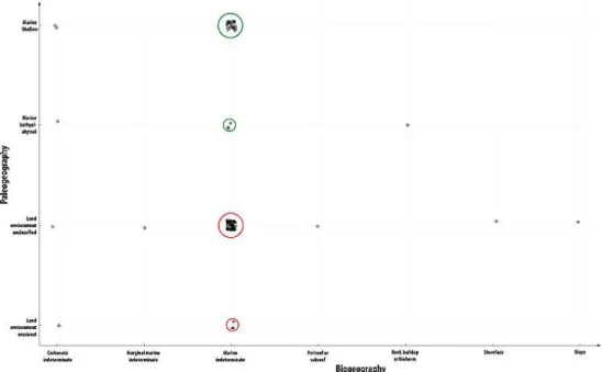
“Land environment unclassified” and the marine fossils (Fig. 7), particularly in Victoria. The fossils have good temporal constraints at Stage level, indicative of Early Devo-nian age, with a number of them more specifically Emsian in age based on conodont horizons – namely Eognathodus trilinearis and Polygnathus dehicens. The Emsian fossils are found in the Bell Point, Buchan Caves and the Waratah Limestones with

5

shell and skeletal fragments. The Early Devonian fauna in central Victoria are found in the Humevale formation containing echinoderm fragments. Unfortunately, there are no wells in the Petroleum Wells Database for this region that penetrate Devonian strata to help further refine the extent of inundation.

3.4 350 Ma (Carboniferous)

10

Shallow marine environments remain along eastern Australia (Langford et al., 2001), and spatially corresponding fossil assemblage data support a marine environment, based on shallow subtidal, carbonate and marine indeterminate indicators at 350 Ma (Fig. 4d). The remaining paleogeography of Australia is largely unclassified, with a re-gion of an erosional environment in Central Australia, coincident with the Alice Springs

15

Orogeny (Langford et al., 2001). Global biogeographic data coverage for this time slice is poor and predominantly indicates marine associated environments.

3.5 300 Ma (Carboniferous – Permian)

Fossil data coverage is poor globally, with only one fossil data point located within the Australian continent at 300 Ma (Fig. 4e). This fossil assemblage indicates a

lacus-20

trine setting, which may be the local base level (sedimentary depocentre) linked to the nearby erosional setting in the paleogeographic model. However insu_fficient paleobiol-ogy data are available to define the extent of the lacustrine environment. Biogeography indicates a deep-water environment off the west coast of Australia, which correlates well with the bathyal-abyssal marine environment in the paleogeographic model.

Inun-25

(10)

BGD

9, 9603–9636, 2012

maps

N. Wright et al.

Title Page

Tables Figures

◭ ◮

Back Close

Full Screen / Esc

Discussion

P

a

per

|

Dis

cussion

P

a

per

|

Discussion

P

a

per

|

Discussio

n

P

a

per

|

Wallaby Zenith Fracture Zone until the separation of Greater India from Australia in the Cretaceous.

3.6 250 Ma (Permo – Triassic boundary)

Biogeographic data coverage is abundant globally, however Australia is poorly rep-resented at this time interval. Based on available biogeographic data, it is indicated

5

Australia has a fluvial-based environment along its present day eastern coast at 250 Ma (Fig. 4f). This correlates with paleogeographic data, which indicates a depo-sitional fluvial-lacustrine environment (Langford et al., 2001), however insufficient bio-geographic data is available to determine the extent and shape with published paleo-geography. The remaining paleogeography of Australia at this time interval is primarily

10

unclassified.

3.7 200 Ma (Triassic – Jurassic)

At this time Australia is located in temperate latitudes (∼30 to 60◦S). Fossil

assem-blages located on the Australian west coast indicate carbonate and “reef, buildup or bioherm” environments at∼200 Ma (Fig. 4g) correlating with the coastal depositional

15

and shallow marine environments in the paleogeography. This is consistent with the rifted margin setting of NW Australia, related to the opening of the Meso- and Neo-Tethys with the detachment of Lhasa and Argoland, respectively, from the northern Gondwana margin.

3.8 150 Ma (Jurassic)

20

(11)

BGD

9, 9603–9636, 2012

maps

N. Wright et al.

Title Page

Tables Figures

◭ ◮

Back Close

Full Screen / Esc

Discussion

P

a

per

|

Dis

cussion

P

a

per

|

Discussion

P

a

per

|

Discussio

n

P

a

per

|

3.9 100 Ma (Cretaceous)

The paleobiology data is more comprehensive for this time interval, and suggests vast expanses of terrestrial environments in the northern hemisphere (100 Ma, Fig. 4i). Fos-sil data indicates two discrete marine and carbonate environments within the present-day Australian continent; located in the north-east (Queensland) and in the centre of

5

the continent (South Australia). The eastern band represented in biogeography indi-cates terrestrial and fluvial environments transitioning into a carbonate marine setting. The paleogeographic descriptor of both areas is unclassified, suggesting that the pa-leogeographic model for this region can be refined with biogeographic indicators. The initiation of Gondwana breakup between Greater India, Australia and Antarctica in the

10

Cretaceous is observed in the propagating inundation of the west Australian margin.

3.10 50 Ma (Paleogene)

Biogeographic indicators are sparse within Australia, and available data suggests ter-restrial, marine and coastal indeterminate environments along the continental margin (50 Ma, Fig. 4j). The paleogeography of Australia is predominantly indicated as an

ero-15

sional land environment, with depositional areas of fluvial environments throughout. The location of biogeographic indicators corresponds to paleogeographic descriptors.

3.11 Recent (Quaternary)

Fossil assemblages in Australia are distributed along the continental margin, and indi-cate coastal, marine, and foreshore environments (Fig. 4k). The Paleogeographic Atlas

20

(12)

BGD

9, 9603–9636, 2012

maps

N. Wright et al.

Title Page

Tables Figures

◭ ◮

Back Close

Full Screen / Esc

Discussion

P

a

per

|

Dis

cussion

P

a

per

|

Discussion

P

a

per

|

Discussio

n

P

a

per

|

4 Discussion

Linking the paleogeographic history of Australia with biogeographic indicators from the Paleobiology Database demonstrates how a paleogeographic model can be tested and potentially improved using empirical, qualitative and quantitative approaches. Highlight-ing associations between the biogeography and paleogeography allowed us to highlight

5

inconsistencies between raw data (fossil collections) and the paleogeographic recon-structions that did not draw upon the global paleobiology during its construction. Al-though the data coverage by paleobiology is imperfect for Australia in comparison to Eurasia and North America, it is an exemplary first-order tool to constrain the evolution of continental inundation histories in the Phanerozoic.

10

4.1 Refining paleogeographic models of Australia using paleobiology

The paleogeographic evolution of Australia is punctuated by a number of significant periods that include the Paleozoic growth of the eastern Australian continent and the inundation of Australia in the mid-Cretaceous from the Late Aptian to the Campanian (Gurnis et al., 1998).

15

4.2 Early Devonian (∼419–393 Ma)

Biogeographic indicators that have a well-defined temporal range and paleo-environmental association can be used to refine existing models of paleogeography. As an example of such an approach, we propose that the inundation of Victoria (VIC) and a portion of New South Wales (NSW) in the Early Devonian lasted until at least the

20

Emsian. We interpret that the marine deposition at the Yass Shelf formed a north-south marine corridor that separated the Snowy Mountains Block from the mainland (Fig. 6b and c). The Devonian outcrops at present-day suggest sedimentation continued into the Emsian, and is largely consistent with the interpretations of Webby (1972) and Veevers (2004) as well as the north-south geometry of the convergent margin along

(13)

BGD

9, 9603–9636, 2012

maps

N. Wright et al.

Title Page

Tables Figures

◭ ◮

Back Close

Full Screen / Esc

Discussion

P

a

per

|

Dis

cussion

P

a

per

|

Discussion

P

a

per

|

Discussio

n

P

a

per

|

eastern NSW in the Paleozoic (Aitchison and Buckman, 2012). Our results indicate that the shallow marine setting persisted until the onset of the Tabberabberan Orogeny (390–380 Ma) in the Middle Devonian (Collins, 2002; Gray and Foster, 1997).

4.3 Cretaceous (145–65 Ma)

The Cretaceous was a significant period of marine inundation in Australia; maximum

5

flooding occurred during the late Aptian to early Albian (120 to 110 Ma) and had pre-dominantly eased by the Campanian (80 to 70 Ma) (Gurnis et al., 1998). Such flooding occurred across large expanses of the continental region east of the cratonic portion of Australia marked by the Tasman Line. Australia experienced maximum flooding in the late Aptian to Early Albian (∼120 to 110 Ma) along the eastern continental

mar-10

gin (Gurnis et al., 1998). The northeastward motion of Australia over a descending Pacific-derived slab induced a strong negative dynamic topography signal that accen-tuated flooding from the mid-Cretaceous sea level highstand (DiCaprio et al., 2009; Gurnis et al., 1998; Heine et al., 2010). Well-constrained models of paleogeography are an important validating mechanism for numerical models of dynamic topography,

15

as demonstrated by Gurnis et al. (1998) in the study of the Cretaceous inundation of Australia (Fig. 8). Subsidence from dynamic topography is distinguishable from loading-induced subsidence as it can be reversed if the negative dynamic topography signal diminishes (Gurnis et al., 1998). In the case of Eastern Australia, a Pacific-derived slab sinking beneath eastern Australia imparts up to 350 m of predicted subsidence from

20

geodynamic models on the region underlying the Eromanga Basin between 120 and 110 Ma, but this effect diminishes by 60 Ma as the depth of the sinking slab increases due to the lower viscous coupling between the slab and the lithosphere. As a result, the inundation of eastern Australia retreated due to_∼200 m of uplift caused by the waning negative dynamic topography signal in an overall eustatic sea level highstand (Seton

25

(14)

BGD

9, 9603–9636, 2012

maps

N. Wright et al.

Title Page

Tables Figures

◭ ◮

Back Close

Full Screen / Esc

Discussion

P

a

per

|

Dis

cussion

P

a

per

|

Discussion

P

a

per

|

Discussio

n

P

a

per

|

deposition>200 m) retreat significantly by 110 Ma (Fig. 8), leaving a shallow marine

setting that disappears by 100 Ma to be replaced by fluvial and other terrestrial de-positional environments. Paleobiology data largely correlates with the paleogeographic model, but suggests that shallow marine settings may have persisted in pockets beyond 100 Ma. Minimal inundation is present at 90 and 80 Ma, and sparse paleobiology data

5

is available for these times, suggesting that the negative dynamic topography signal diminished by∼100 Ma or that eustatic sea levels fell to induce a marine regression.

Additionally, the inundation history is recorded in the fossil collections from the Ero-manga Basin, with a distinct peak of fossil preservation coinciding with the Cretaceous inundation (Fig. 9).

10

4.4 Testing plate motions using paleogeography and biogeography

Paleogeography and biogeography embedded within plate reconstructions can be used to uncover inconsistencies and help refine the plate motion model. The Cretaceous pe-riod records significant changes in the tectonic forces acting on the Australian plate, largely driven by the breakup of Gondwana and the subduction of Pacific material

15

along Australia’s eastern margin (Veevers, 2012). The relative plate motions suggest rifting between Australia and Greater India began at∼165 Ma, consistent with

inter-pretations of seismic sections that indicate rift-related normal faulting penetrated Late Jurassic sedimentary sequences (Song and Cawood, 2000) and syn-rift sediments in the southern Perth Basin (Veevers, 2012). However, the rift-related inundation of this

20

margin occurs much later at∼139 Ma based on the paleogeographic model. The

dis-crepancy between the Late Jurassic onset of rifting and delayed submergence may be accounted for by the oblique style or rifting, which resulted in abundant strike-slip fault-ing (Song and Cawood, 2000), and therefore relatively little lithospheric extension for much of the rift phase, thus delaying subsidence and inundation until a few million years

25

before breakup. Additionally, seafloor spreading initiated some time between∼136 and

(15)

BGD

9, 9603–9636, 2012

maps

N. Wright et al.

Title Page

Tables Figures

◭ ◮

Back Close

Full Screen / Esc

Discussion

P

a

per

|

Dis

cussion

P

a

per

|

Discussion

P

a

per

|

Discussio

n

P

a

per

|

Although the plate motion model is consistent with the rifting history between Australia-India-Antarctica, Golonka’s (2007) plate motion model may need refinement for the Cretaceous Australia-Antarctica rifting history. The paleogeographic model sug-gests that inundation of the western Australia-Antarctic margin initiates by 125 Ma and propagates eastward, reaching Tasmania by 100 Ma, consistent with a previous onset

5

of rifting in the Valanginian (Totterdell and Bradshaw, 2004). The progressive submer-gence of the margin reflects the eastward propagation of the rift, as originally sug-gested by Mutter et al. (1985), that may be accentuated by the global mid-Cretaceous seafloor spreading pulse resulting in a eustatic sea level highstand (Seton et al., 2009). However, the peak of the sea level highstand and seafloor spreading pulse post-dates

10

the peak inundation of the rifted Australia-Antarctica margin, and suggests that the pro-gressive inundation was mainly rift-related. The pre-breakup fit in the Golonka (2007) model requires refinement to minimise continental overlaps and initiation of rifting at

∼121 Ma as demonstrated by Williams et al. (2011) for the Australian-Antarctic

conju-gate margins.

15

The pre-breakup fit between Greater India and western Australia, and in particular the extent of Greater India, is another long-standing controversy that can be viewed in the context of paleogeography (Fig. 9). The proponents of a maximum-extent Greater India suggest that the limit of this margin extended to the northern Exmouth Plateau at pre-breakup fit (Lee and Lawver, 1995; van Hinsbergen et al., 2011), while

alterna-20

tive models propose a smaller Greater India bound by the present-day geometry of the Wallaby-Zenith Fracture Zone (Ali and Aitchison, 2005; Klootwijk and Conaghan, 1979; Replumaz et al., 2004; Zahirovic et al., 2012; Gibbons et al., 2012). Our plate recon-structions with combined biogeography and paleogeography indicate that inundation of the western Australian margin did not extend south of the Wallaby-Zenith Fracture

25

Zone until the final breakup of India from Australia in the Cretaceous (Fig. 10). This suggests that the Greater Indian continental margin extended no more than∼1000 km

(16)

BGD

9, 9603–9636, 2012

maps

N. Wright et al.

Title Page

Tables Figures

◭ ◮

Back Close

Full Screen / Esc

Discussion

P

a

per

|

Dis

cussion

P

a

per

|

Discussion

P

a

per

|

Discussio

n

P

a

per

|

resulted from a thinned and submerged large Greater India, the north-westward de-tachment of terranes from NW Australia would have generated a narrow continental margin along northern Greater India along transforms similar in orientation to those in the Argo Abyssal Plain (Heine and M ¨uller, 2005) and analogous to the narrow conti-nental margin resulting from the shearing along the Romanche Fracture Zone and the

5

Benue Trough between Ghana and Nigeria (Basile et al., 1993; Bonatti et al., 1994).

4.5 Data coverage and resolution

Data coverage of the eastern coast of Australia, follow the band of Cretaceous inunda-tion, resulting in reasonable spatio-temporal coverage of the region (Figs. 5 and 10). At least five sizeable gaps in the temporal coverage are present in the paleobiology

10

and we suggest that some of the temporal gaps are a result of the episodic orogenic events related to the Tasman Orogenic System in the Paleozoic, leading to the east-ward growth of the Australian continent in an accretionary convergent margin setting (Coney et al., 1990; Crawford et al., 2003; Henderson et al., 2011; Solomon and Grif-fiths, 1972). The lack of fossil assemblages elsewhere in Australia is a result of biased

15

sampling and the environment type at the time. The combination of paleobiology, plate reconstructions and the paleogeography inGPlateshas allowed us to use a novel ap-proach to test the correlation of existing paleogeographic maps and fossil indicators of environments. The use ofGPlates is significant, as paleogeographic maps can be dynamic and updated with relative ease based on new data, rather than the reliance

20

on static maps that are revised infrequently. GPlates also allows the incorporation of multiple layers of proxy data to increase the confidences of paleogeographic recon-structions. The development of such interactive maps can be applied to other areas of geodynamic modelling, due to the technological capabilities demonstrated byGPlates. Spatio-temporal data coverage is a considerable concern in the interpretation of the

25

(17)

BGD

9, 9603–9636, 2012

maps

N. Wright et al.

Title Page

Tables Figures

◭ ◮

Back Close

Full Screen / Esc

Discussion

P

a

per

|

Dis

cussion

P

a

per

|

Discussion

P

a

per

|

Discussio

n

P

a

per

|

day southern hemisphere, such as Australia. Such discrepancies may be the result of biased sampling and/or preservation and environmental conditions at the time of depo-sition. Global data coverage is relatively poor for times before the Carboniferous; this may be attributed to the poor preservation of organisms. Spatio-temporal data cover-age in Australia has predominantly been restricted to eastern Australia, and suggests at

5

least five temporal gaps in coverage (Fig. 10). Paleogeographic reconstructions were further restricted by the lack of variation in fossil assemblage environments: paleo-biology data are predominantly available for marine paleoenvironments. As a result, other proxy data are required for constraining paleoenvironments with low biological preservation potential – such as orogenic settings that can be constrained using

meta-10

morphic assemblages and denudation histories in proximal basins. Paleogeographic maps can be further refined by incorporating additional published paleoenvironment indicators, including well logs and other time-dependent datasets usingGPlates. Fu-ture directions include a greater analysis of paleogeography on a global scale as indi-cated by biogeography, including the effect of glaciations, continental inundations and

15

mass extinction throughout the Phanerzoic on fossil assemblages. In particular, such an approach would be best suited for European and North American paleogeographic reconstructions due to the higher spatio-temporal coverage in the fossil record (Han-nisdal and Peters, 2011).

Glaciations have played a major role in global climate throughout the Phanerozoic,

20

and may have influenced the preservation of organisms. The glaciation throughout the latest Devonian to Early Permian (Scotese et al., 1999) may be responsible for the few and scattered fossil assemblages found globally in the Late Paleozoic. Similarly, the inundation of continental regions can influence preservation of organisms, based on the availability of desirable preservation conditions, and should be noted in global and

25

(18)

BGD

9, 9603–9636, 2012

maps

N. Wright et al.

Title Page

Tables Figures

◭ ◮

Back Close

Full Screen / Esc

Discussion

P

a

per

|

Dis

cussion

P

a

per

|

Discussion

P

a

per

|

Discussio

n

P

a

per

|

spatial and temporal fossil preservation in the eastern Australian basins (Fig. 10). The increased inundation of the continent and a biased biological preservation during this time interval is consistent with a mid-Cretaceous seafloor spreading pulse and increase in eustatic sea levels (Seton et al., 2009).

5 Conclusions

5

Our approach demonstrates that paleogeographic and plate reconstructions can be improved and refined using biogeographic indicators from the global Paleobiology Database. Our novel application of spatio-temporal data mining can be used to iden-tify inconsistencies between paleogeography and biogeography. Our approach allows the incorporation of multiple proxy datasets to help refine plate and paleogeographic

10

reconstructions, and enables the creation of a new generation of digital and interac-tive models that allow users to create dynamic maps that are expandable and testable that take advantage of regularly maintained databases such as the global paleobiology. Sediments and related fossil assemblages are largely confined to basins and this only provides indirect constraints for elevated topographic regions representing sediment

15

sources. As a result, in the future it will be desirable to incorporate proxies of eleva-tion, such as paleo-altimetry estimates based on paleobiological indicators (i.e. leaf morphologies and stomata densities) (McElwain, 2004), and stable and metamorphic assemblages isotopes (Blisniuk and Stern, 2005).GPlatesis evolving into an open in-novation platform with a plugin infrastructure and an extended information model that

20

(19)

BGD

9, 9603–9636, 2012

maps

N. Wright et al.

Title Page

Tables Figures

◭ ◮

Back Close

Full Screen / Esc

Discussion

P

a

per

|

Dis

cussion

P

a

per

|

Discussion

P

a

per

|

Discussio

n

P

a

per

|

Supplementary material related to this article is available online at: http://www.biogeosciences-discuss.net/9/9603/2012/

bgd-9-9603-2012-supplement.zip.

Acknowledgements. The project was supported by ARC grants FL0992245 and DP0987713. Thomas Landgrebe provided help with the data mining methodology. This is Paleobiology 5

Database publication #163.

References

Aitchison, J. C. and Buckman, S.: Accordion vs. quantum tectonics: Insights into continental growth processes from the Paleozoic of eastern Gondwana, Gondwana Res., 22, 674–680, 2012.

10

Ali, J. R. and Aitchison, J. C.: Greater India, Earth-Sci. Rev., 72, 169–188, 2005.

Basile, C., Mascle, J., Popoff, M., Bouillin, J., and Mascle, G.: The Ivory Coast-Ghana transform margin: A marginal ridge structure deduced from seismic data, Tectonophysics, 222, 1–19, 1993.

Blisniuk, P. M. and Stern, L. A.: Stable isotope paleoaltimetry: A critical review, Am. J. Sci., 305, 15

1033–1074, 2005.

Bonatti, E., Ligi, M., Gasperini, L., Peyve, A., Raznitsin, Y., and Chen, Y.: Transform migration and vertical tectonics at the Romanche fracture zone, equatorial Atlantic, J. Geophys. Res., 99, 21779–21802, doi:10.1029/94JB01178, 1994.

Cocks, L. R. M. and Torsvik, T. H.: Earth geography from 500 to 400 million years ago: a faunal 20

and palaeomagnetic review, J. Geol. Soc. London, 159, 631–644, 2002.

Collins, W. J.: Nature of extensional accretionary orogens, Tectonics, 21, 1024, doi:10.1029/2000TC001272, 2002.

Coney, P. J., Edwards, A., Hine, R., Morrison, F., and Windrim, D.: The regional tectonics of the Tasman orogenic system, eastern Australia, J. Struct. Geol., 12, 519–543, 1990.

25

(20)

BGD

9, 9603–9636, 2012

maps

N. Wright et al.

Title Page

Tables Figures

◭ ◮

Back Close

Full Screen / Esc

Discussion

P

a

per

|

Dis

cussion

P

a

per

|

Discussion

P

a

per

|

Discussio

n

P

a

per

|

DiCaprio, L., Gurnis, M., and M ¨uller, R. D.: Long-wavelength tilting of the Australian continent since the Late Cretaceous, Earth Planet. Sci. Lett., 278, 175–185, 2009.

Donnadieu, Y., Godd ´eris, Y., Pierrehumbert, R., Dromart, G., Fluteau, F., and Jacob, R.: A GEOCLIM simulation of climatic and biogeochemical consequences of Pangea breakup, Geochem. Geophy. Geosy., 7, Q11019, doi:10.1029/2006GC001278, 2006.

5

Ford, D. and Golonka, J.: Phanerozoic paleogeography, paleoenvironment and lithofacies maps of the circum-Atlantic margins, Mar. Petrol. Geol., 20, 249–285, 2003.

Gibbons, A. D., Barckhausen, U., van den Bogaard, P., Hoernle, K., Werner, R., Whit-taker, J. M., and M ¨uller, R. D.: Constraining the Jurassic extent of Greater India: Tec-tonic evolution of the West Australian margin, Geochem. Geophy. Geosy., 13, Q05W13, 10

doi:10.1029/2011GC003919, 2012.

Golonka, J.: Late Triassic and Early Jurassic palaeogeography of the world, Palaeogeogr. Palaeocl., 244, 297–307, 2007.

Golonka, J., Krobicki, M., Pajak, J., Van Giang, N., and Zuchiewicz, W.: Global Plate Tectonics and Paleogeography of Southeast Asia, edited by: Doktor, M., Faculty of Geology, Geo-15

physics and Environmental Protection, AGH University of Science and Technology, Arkadia, Krakow, 128 pp., 2006.

Gray, D. R. and Foster, D. A.: Orogenic concepts-application and definition: Lachlan Fold Belt, eastern Australia, Am. J. Sci., 297, 859–891, 1997.

Gurnis, M., Muller, R. D., and Moresi, L.: Cretaceous vertical motion of Australia and the 20

Australian-Antarctic discordance, Science, 279, 1499–1504, 1998.

Gyllenhaal, E. D., Engberts, C. J., Markwick, P. J., Smith, L. H., and Patzkowsky, M. E.: The Fujita-Ziegler model: a new semi-quantitative technique for estimating paleoclimate from pa-leogeographic maps, Palaeogeogr. Palaeocl., 86, 41–66, 1991.

Hallam, A. and Cohen, J.: The case for sea-level change as a dominant causal factor in mass 25

extinction of marine invertebrates [and discussion], Philos. T. Roy. Soc. B, 325, 437–455, 1989.

Hallam, A. and Wignall, P.: Mass extinctions and sea-level changes, Earth-Sci. Rev., 48, 217– 250, 1999.

Hannisdal, B. and Peters, S. E.: Phanerozoic Earth System Evolution and Marine Biodiversity, 30

Science, 334, 1121–1124, 2011.

(21)

BGD

9, 9603–9636, 2012

maps

N. Wright et al.

Title Page

Tables Figures

◭ ◮

Back Close

Full Screen / Esc

Discussion

P

a

per

|

Dis

cussion

P

a

per

|

Discussion

P

a

per

|

Discussio

n

P

a

per

|

Heine, C., M ¨uller, R. D., Steinberger, B., and DiCaprio, L.: Integrating deep Earth dy-namics in paleogeographic reconstructions of Australia, Tectonophysics, 483, 135–150, doi:10.1016/j.tecto.2009.08.028, 2010.

Henderson, R. A., Innes, B. M., Fergusson, C. L., Crawford, A. J., and Withnall, I. W.: Collisional accretion of a Late Ordovician oceanic island arc, northern Tasman Orogenic Zone, Australia, 5

Aust. J. Earth Sci., 58, 1–19, doi:10.1080/08120099.2010.535564, 2011.

Klootwijk, C. and Conaghan, P.: The extent of Greater India, I. Preliminary palaeomagnetic data from the Upper Devonian of the eastern Hindukush, Chitral (Pakistan), Earth Planet. Sci. Lett., 42, 167–182, 1979.

Langford, R. P., Wilford, G. E., Truswell, E. M., Totterdell, J. M., Yeung, M., Isem, A. R., Yeates, 10

A. N., Bradshaw, M., Brakel, A. T., Olissoff, S., Cook, P. J., and Strusz, D. L.: Palaeogeo-graphic Atlas of Australia, Geoscience Australia, 2001.

Lee, T. Y. and Lawver, L. A.: Cenozoic plate reconstruction of Southeast Asia, Tectonophysics, 251, 85–138, 1995.

McElwain, J. C.: Climate-independent paleoaltimetry using stomatal density in fossil leaves as 15

a proxy for CO₂partial pressure, Geology, 32, 1017–1020, 2004.

Metcalfe, I.: Gondwanaland origin, dispersion, and accretion of East and Southeast Asian con-tinental terranes, J. S. Am. Earth Sci., 7, 333–347, 1994.

Miller, K. G., Kominz, M. A., Browning, J. V., Wright, J. D., Mountain, G. S., Katz, M. E., Sug-arman, P. J., Cramer, B. S., Christie-Blick, N., and Pekar, S. F.: The phanerozoic record of 20

global sea-level change, Science, 310, 1293–1298, 2005.

M ¨uller, R. D., Sdrolias, M., Gaina, C., Steinberger, B., and Heine, C.: Long-term sea-level fluc-tuations driven by ocean basin dynamics, Science, 319, 1357–1362, 2008.

Mutter, J. C., A Hegarty, K., Cande, S. C., and Weissel, J. K.: Breakup between Australia and Antarctica: a brief review in the light of new data, Tectonophysics, 114, 255–279, 1985. 25

Replumaz, A., Karason, H., van der Hilst, R., Besse, J., and Tapponnier, P.: 4-D evolution of SE Asia’s mantle from geological reconstructions and seismic tomography, Earth Planet. Sci. Lett., 221, 103–115, 2004.

Robb, M. S., Taylor, B., and Goodli_ffe, A. M.: Re-examination of the magnetic lineations of the Gascoyne and Cuvier Abyssal Plains, offNW Australia, Geophys. J. Int., 163, 42–55, 2005. 30

(22)

BGD

9, 9603–9636, 2012

maps

N. Wright et al.

Title Page

Tables Figures

◭ ◮

Back Close

Full Screen / Esc

Discussion

P

a

per

|

Dis

cussion

P

a

per

|

Discussion

P

a

per

|

Discussio

n

P

a

per

|

Scotese, C. R., Boucot, A. J., and McKerrow, W. S.: Gondwanan palaeogeography and palaeo-climatology, J. Afr. Earth Sci., 28, 99–114, 1999.

Seton, M., Gaina, C., M ¨uller, R., and Heine, C.: Mid-Cretaceous seafloor spreading pulse: Fact or fiction?, Geology, 37, 687–690, 2009.

Seton, M., M ¨uller, R., Zahirovic, S., Gaina, C., Torsvik, T., Shephard, G., Talsma, A., Gurnis, M., 5

Turner, M., and Chandler, M.: Global continental and ocean basin reconstructions since 200 Ma, Earth-Sci. Rev., 113, 212–270, 2012.

Sikora, P. J., Ogg, J. G., Gary, A., Cervato, C., Gradstein, F., Huber, B. T., Marshall, C., Stein, J. A., and Wardlaw, B.: An integrated chronostratigraphic data system for the twenty-first century, in: Geoinformatics: data to knowledge, 397, 53–59, 2006.

10

Solomon, M. and Griffiths, J.: Tectonic evolution of the Tasman Orogenic zone, eastern Aus-tralia, Nature, 237, 3–6, 1972.

Song, T. and Cawood, P. A.: Structural styles in the Perth Basin associated with the Mesozoic break-up of Greater India and Australia, Tectonophysics, 317, 55–72, 2000.

Stanley, S. M.: Paleozoic mass extinctions; shared patterns suggest global cooling as a com-15

mon cause, Am. J. Sci., 288, 334–352, doi:10.2475/ajs.288.4.334, 1988.

Torsvik, T. and van der Voo, R.: Refining Gondwana and Pangea Palaeogeography: Estimates of Phanerozoic non dipole (octupole) fields, Geophys. J. Int., 151, 771–794, 2002.

Totterdell, J. and Bradshaw, B.: The structural framework and tectonic evolution of the Bight Basin, Eastern Australasian Basins Symposium II, Adelaide, 41–61, 2004.

20

van der Voo, R.: The reliability of paleomagnetic data, Tectonophysics, 184, 1–9, 1990. van Hinsbergen, D. J. J., Kapp, P., Dupont-Nivet, G., Lippert, P. C., DeCelles, P. G., and Torsvik,

T. H.: Restoration of Cenozoic deformation in Asia and the size of Greater India, Tectonics, 30, TC5003, doi:10.1029/2011TC002908, 2011.

Veevers, J. J.: Gondwanaland from 650–500 Ma assembly through 320 Ma merger in Pangea 25

to 185–100 Ma breakup: supercontinental tectonics via stratigraphy and radiometric dating, Earth-Sci. Rev., 68, 1–132, doi:10.1016/j.earscirev.2004.05.002, 2004.

Veevers, J. J.: Reconstructions before rifting and drifting reveal the geological connections be-tween Antarctica and its conjugates in Gondwanaland, Earth-Sci. Rev., 111, 249–318, 2012. Webby, B. D.: Devonian geological history of the Lachlan Geosyncline, J. Geol. Soc. Aust., 19, 30

99–123, 1972.

(23)

BGD

9, 9603–9636, 2012

maps

N. Wright et al.

Title Page

Tables Figures

◭ ◮

Back Close

Full Screen / Esc

Discussion

P

a

per

|

Dis

cussion

P

a

per

|

Discussion

P

a

per

|

Discussio

n

P

a

per

|

Williams, S. E., Whittaker, J. M., and M ¨uller, R. D.: Full-fit, palinspastic reconstruction of the conjugate Australian-Antarctic margins, Tectonics, 30, TC6012, doi:10.1029/2011TC002912, 2011.

Zahirovic, S., M ¨uller, R. D., Seton, M., Flament, N., Gurnis, M., and Whittaker, J.: Insights on the kinematics of the India-Eurasia collision from global geodynamic models, Geochem. Geophy. 5

(24)

BGD

9, 9603–9636, 2012

maps

N. Wright et al.

Title Page Abstract Introduction Conclusions References Tables Figures ◭ ◮ ◭ ◮ Back Close

Full Screen / Esc

Printer-friendly Version Interactive Discussion Discussion P a per | Dis cussion P a per | Discussion P a per | Discussio n P a per |

Table 1.Paleogeographic descriptors in the Paleogeographic Atlas of Australia (Langford et al., 2001) and colour (RGB) values representing each environment.

Paleoenvironment Descriptor RGB

Code

Mar

ine

Bathyal-Abyssal and Abyssal

Deep water sediments including condensed sequences, turbidites and shales indicative of water depths exceeding 200 m.

22/253/255 and 20/209/253

Shallow Sediments deposited on continental shelves

including sand, mud and limestone indicative of 20 to 200 m watch depths.

159/255/255

Very Shallow Sediments deposited above wave base including

oolitic and cross-bedded deposits indicative of 0 to 20 m water depths.

228/255/253

Coastal deposi-tional deltaic

Protruding lobate outline of sedimentary extent. 224/247/218

Coastal deposi-tional paralic

Environments representing land-sea interface including lagoonal, estuarine, beach and intertidal sediments. Facies including cross-bedded beach sands and finely laminated organic sediments.

224/247/142

Coastal

Depositional fluvial

Alluvial river deposits of braided and meandering streams, dominated by sandy sediment and coarser sediment.

255/239/163

Depositional fluvial-lacustrine

Low energy depositional environments of fine grain sediment (including coal) such as in river channels, swamps, floodplains and shallow lakes.

234/201/162

Land

Depositional erosional

Erosional regions with higher relief based on paleo-currents, volcanic activity and tectonic setting.

237/185/174

Depositional unclassified

No preserved sediments of age representing paleogeographic reconstruction.

248/243/237

Glacial Sediments including glacial tillite and dropstones

indicative of glacier movement and transport.

(25)

BGD

9, 9603–9636, 2012

maps

N. Wright et al.

Title Page

Tables Figures

◭ ◮

Back Close

Full Screen / Esc

Discussion

P

a

per

|

Dis

cussion

P

a

per

|

Discussion

P

a

per

|

Discussio

n

P

a

per

|

(26)

BGD

9, 9603–9636, 2012

maps

N. Wright et al.

Title Page

Tables Figures

◭ ◮

Back Close

Full Screen / Esc

Discussion

P

a

per

|

Dis

cussion

P

a

per

|

Discussion

P

a

per

|

Discussio

n

P

a

per

|

(27)

BGD

9, 9603–9636, 2012

maps

N. Wright et al.

Title Page

Tables Figures

◭ ◮

Back Close

Full Screen / Esc

Discussion

P

a

per

|

Dis

cussion

P

a

per

|

Discussion

P

a

per

|

Discussio

n

P

a

per

|

Fig. 3. Fossil collections (A) and the Australian paleogeography (B) are reconstructed in

(28)

BGD

9, 9603–9636, 2012

maps

N. Wright et al.

Title Page

Tables Figures

◭ ◮

Back Close

Full Screen / Esc

Discussion

P

a

per

|

Dis

cussion

P

a

per

|

Discussion

P

a

per

|

Discussio

n

P

a

per

|

(29)

BGD

9, 9603–9636, 2012

maps

N. Wright et al.

Title Page

Tables Figures

◭ ◮

Back Close

Full Screen / Esc

Discussion

P

a

per

|

Dis

cussion

P

a

per

|

Discussion

P

a

per

|

Discussio

n

P

a

per

|

(30)

BGD

9, 9603–9636, 2012

maps

N. Wright et al.

Title Page

Tables Figures

◭ ◮

Back Close

Full Screen / Esc

Discussion

P

a

per

|

Dis

cussion

P

a

per

|

Discussion

P

a

per

|

Discussio

n

P

a

per

|

(31)

BGD

9, 9603–9636, 2012

maps

N. Wright et al.

Title Page

Tables Figures

◭ ◮

Back Close

Full Screen / Esc

Discussion

P

a

per

|

Dis

cussion

P

a

per

|

Discussion

P

a

per

|

Discussio

n

P

a

per

|

(32)

BGD

9, 9603–9636, 2012

maps

N. Wright et al.

Title Page

Tables Figures

◭ ◮

Back Close

Full Screen / Esc

Discussion

P

a

per

|

Dis

cussion

P

a

per

|

Discussion

P

a

per

|

Discussio

n

P

a

per

|

(33)

BGD

9, 9603–9636, 2012

maps

N. Wright et al.

Title Page

Tables Figures

◭ ◮

Back Close

Full Screen / Esc

Discussion

P

a

per

|

Dis

cussion

P

a

per

|

Discussion

P

a

per

|

Discussio

n

P

a

per

|

(34)

BGD

9, 9603–9636, 2012

maps

N. Wright et al.

Title Page

Tables Figures

◭ ◮

Back Close

Full Screen / Esc

Discussion

P

a

per

|

Dis

cussion

P

a

per

|

Discussion

P

a

per

|

Discussio

n

P

a

per

|