www.nonlin-processes-geophys.net/15/591/2008/ © Author(s) 2008. This work is distributed under the Creative Commons Attribution 3.0 License.
Nonlinear Processes
in Geophysics
A propagation-separation approach to estimate the autocorrelation
in a time-series
D. V. Divine1,*, J. Polzehl2, and F. Godtliebsen3
1Department of Mathematics and Statistics, Faculty of Science, University of Tromsø, 9037, Norway 2Weierstrass Institute for Applied Analysis and Stochastics, Mohrenstr. 39, 10117 Berlin, Germany 3Department of Mathematics and Statistics, Faculty of Science, University of Tromsø, 9037, Norway *also at: Norwegian Polar Institute, Polar Environmental Centre, 9296 Tromsø, Norway
Received: 22 October 2007 – Revised: 12 June 2008 – Accepted: 19 June 2008 – Published: 23 July 2008
Abstract. The paper presents an approach to estimate pa-rameters of a local stationary AR(1) time series model by maximization of a local likelihood function. The method is based on a propagation-separation procedure that leads to data dependent weights defining the local model. Using free propagation of weights under homogeneity, the method is ca-pable of separating the time series into intervals of approx-imate local stationarity. Parameters in different regions will be significantly different. Therefore the method also serves as a test for a stationary AR(1) model. The performance of the method is illustrated by applications to both synthetic data and real time-series of reconstructed NAO and ENSO indices and GRIP stable isotopes.
1 Introduction
A frequent use of the first order autoregressive model, AR(1), in climate applications is conditioned by its simplicity and ef-ficiency in capturing the inertial nature of climatic phenom-ena (Hasselmann, 1976). Whereas a choice of a global para-metric structure for the fitted model is common, it is often worthwhile to know whether such an approximation provides an adequate description of the analyzed series. This can be-come an issue, for example, in null hypothesis testing, when the fitted model is used to assess whether or not the variabil-ity recorded in a time series is consistent with a stochastic origin of this type.
In this paper we propose a method which, using the idea of structural adaptation, is capable of isolating the periods in the analyzed data where the parameters of the fitted AR(1)
Correspondence to: D. V. Divine
model differ significantly. The method is largely based on ideas implemented in the adaptive weight smoothing (AWS) procedure for local constant modeling, introduced earlier in (Polzehl and Spokoiny, 2000) in the context of image denois-ing. The AWS technique was later successfully generalized to the case of an arbitrary local linear parametric structure (Chen et al., 2008) and extended to a broad class of nonpara-metric models, including e.g. the regression, density, Pois-son and binary response model. The same idea was applied to estimation of the tail index parameter, classification, den-sity and volatility estimation (Polzehl and Spokoiny, 2002). Theoretical results for exponential families were achieved in (Polzehl and Spokoiny, 2006).
The paper is presented as follows. In Sect. 2 we recall a global likelihood approach to the estimation of the sought parameters in the AR(1) model. Section 3 introduces the con-cept of local likelihood. A definition of weights is given in Sect. 4. Sections 5 and 6 present a numerical implementation of the method and explain the choice of parameters used, re-spectively. Examples demonstrating the performance of the method are shown in Sect. 7 followed by brief conclusions in Sect. 8.
2 Global likelihood estimation
The model of the discrete AR(1) process is formulated as
yi =φyi−1+ǫi, i=1, ..., n (1)
whereφ is the autoregressive parameter, yi is the ith
ob-served realization of the AR(1) process and ǫi are
Given parametersφandσ2, the likelihood function of the vectorY =(y1, ..., yn)has the form (Brockwell and Davis,
1998) (see 8.7.2-4):
L(Y|φ, σ2)=(2π σ2)−n2×
×exp
− 1 2σ2(a1φ
2+(1+φ2)a
2+a3−2φa4)
(2) where
a1=y12 a2=Pnj−1=2yj2
a3=yn2 a4=
Pn
j=2yjyj−1
(3)
The global maximum likelihood estimates forφ andσ2
are defined by maximization of the log-likelihood function log(L(Y|φ, σ2)). Solving
∂(logL(Y))
∂σ2 =
∂(logL(Y))
∂φ =0 (4)
forσ2andφyields after some algebra approximative likeli-hood estimates ofφandσ2given as
ˆ
φ= a4
a2+a1
; cσ2= a2+a3−2φaˆ 4
n . (5)
The asymptotic variance estimates of the model parame-ters can be determined using the Fisher information matrix for the log-likelihood logL(Y|φ, σ2). Using the expecta-tions E(a1) = E(a3) = σ
2
1−φ2 , E(a2) =
(n−2)σ2
1−φ2 and
E(a4)= (n−1)φσ
2
1−φ2 this leads to
Iφ,σ2 = −Eφ,σ2
∂2logL(Y|φ,σ2) (∂φ)2
∂2logL(Y|φ,σ2) ∂φ∂σ2
∂2logL(Y|φ,σ2) ∂φ∂σ2
∂2logL(Y|φ,σ2) (∂σ2)2
=
n−1 1−φ2 0
0 n−2
2σ4
!
(6)
InvertingIφ,σ2 yields the asymptotic covariance matrix for
{φ, σ2}as
I−1
φ,σ2 =
1−φ2
n−1 0
0 n2σ−24
!
. (7)
Respective asymptotic confidence intervals (CI) forφˆandbσ2
can now be obtained employing the asymptotic normality of the estimates.
3 Local likelihood and its estimation using structural adaptation
A global parametric structure considered in the previous section is generally too restrictive. To allow for possible variability in the model coefficients we introduce a local parametric structure to the model. The most general way of describing a local model is based on weights assigned to each observation used. Let, for a fixed t, a nonneg-ative weight wi=wi(t )≤1 be assigned to the observations
yi atti, i=1, .., n. The local, or weighted, maximum
log-likelihood estimate is, in this case, introduced as
n
ˆ
φ(t ),bσ2(t )o=arg supφ,σ2
n X
i=1
wi(t )logp(yi|φ, σ2)
where logp(yi|φ, σ2)denotes the contribution to the global log-likelihood function at any given pointti, given by
logp(yi|φ, σ2)= −1
2log(2π σ
2)− (8)
− 1
2σ2(yi −φyi−1)
2; i=2, ..., n.
The principal idea of the approach proposed in (Polzehl and Spokoiny, 2000) is to use a structural assumption of lo-cal homogeneity to determine data dependent weightswi(tj)
that define the local likelihood. Weightswi(tj)are obtained
using a sequence of likelihood ratio tests for the hypothesis that the parameters at timestj andti coincide.
For any local model characterized by a set of weights
W (t )=(w1(t ), ..., wn(t )), the local log-likelihood defined by
these weights is
L(W (t ), φ, σ2)= −N (t )
2 log(2π σ
2)− (9)
− 1
2σ2(R1(t )+φ 2R
2(t )−2φS(t )),
were
N (t )=
n X
j=1
wj(t ); S(t )=
n X
j=1
wj(t )yjyj−1;
R1(t )=
n X
j=2
wj(t )yj2; R2(t )=
n X
j=2
wj(t )y2j−1. (10)
Maximization of this weighted log-likelihood with respect to
φandσ2yields the local Maximum Likelihood estimates
ˆ
φ(t )= S(t )
R2(t )
and bσ2(t )=R1(t )R2(t )−S(t )
2
N (t )R2(t )
. (11)
Let us assume that the time series is stationary within some local vicinity U (ti)of time ti. If we knew the
knowledge is usually not available, but information on a suitable local modelW (ti)can be inferred from estimates n
ˆ
φ(t ),bσ2(t )
o
. Assume that we have estimates in all ob-served time pointstj. We can use this information to infer
on the neighborhoodU (ti)by testing the hypothesis
H:nφ (ti), σ2(ti)
o
=nφ (tj), σ2(tj)
o
. (12)
A weightwij can be assigned based on the value of a test
statistic Tij, assigning zero weights if
φ (ti), σ2(ti) and
φ (tj), σ2(tj) are significantly different.
This can be embedded into an iterative procedure. At each iteration (k) we restrict positive weights to observations at timestj with|tj−ti|<h(k), starting with a very small initial
bandwidth(h(0))and increasing the bandwidth with each it-eration. Testing along the entire time-series yields a set of weightsW (ti)that determines a local model inti and hence
a new estimate ofφ (t ), σ2(t ) inti.
We define a test statisticsTij by a local likelihood ratio test for the hypothesis of equal parameters at timesti andtj. Given estimates
n
ˆ
φi,σˆi2
o
and
n
ˆ
φj,σˆj2
o
at timestiandtj, the
difference between the local log-likelihoods evaluated for the two estimates employing the weighting schemeWiis
Tij =L(W,φˆi,σˆi2,φˆj,σˆj2)
= Ni 2 log(
ˆ
σj2
ˆ
σi2)−R1i(
1 2σˆi2 −
1 2σˆj2)− − 1
2σˆi2( ˆ
φi2R2i −2φˆiSi)+
1 2σˆj2(
ˆ
φj2R2i −2φˆjSi). (13)
The value ofTij is used to define a statistical penalty. That
is, ifTij is sufficiently larger than some prescribed valueλ,
the parameters at timetiandtjare significantly different and
therefore the corresponding weight is set to zero. The pro-cess of finding the local models and estimating the local like-lihoods is implemented in an iterative procedure, formally presented below in Sect. 5.
Approximate confidence limits for the parametersφ, σ2
at everyti can be established using an equivalent of Eq. (7) for the local likelihood and assuming asymptotic normality of the estimates. This yields approximate variances ofφ(t )ˆ
andσˆ2(t )as
Vφ(t )=
Pn
j=2wj(t )2
N (t )2 (1− ˆφ(t )
2) and
Vσ2(t )=
Pn
j=2wj(t )2
N (t )2 2σˆ
4(t ) (14)
The correspondent 100(1 −α)% CIs are given by φ(t )ˆ ±
Zα/2
p
Vφ(t )andbσ2(t )±Zα/2
p
Vσ2(t )onφ(t )ˆ andbσ2(t ),
re-spectively, whereZα/2denotes theα/2 quantile of the
stan-dard Gaussian distribution. These intervals are approxima-tive in the sense that they are centered at mean parameter val-ues within the set of time points with positive weightswi(tj).
They are, as usual for any nonparametric estimates, not ad-justed for a potential bias. Additionally the asymptotic for
σ2is very slow.
Note that in a homogeneous situation with a free exten-sion of every local model during the iterative process, local MLE’s
n
ˆ
φ(t ),bσ2(t )
o
and their variances converge asymptot-ically to their global MLE estimates, as given by Eqs. 5 and 7.
4 Definition of weights
For every pair (i, j ), the weight wij is constructed on the base of two independent quantities: a location penalty
lij=
ρ(ti, tj)/ h 2
and a statistical penaltysij(k)=Tij/λ. Here handρ(ti, tj)=|ti−tj| denote, respectively, the bandwidth
and the Euclidean distance between the design pointsti and tj. The parameterλcan be treated as the critical value for the
test statisticsTij and defined empirically to satisfy a
propa-gation criteria in the homogeneous case (see below). The weights are thereby defined as
wij =Kloc(lij)Kst(sij) (15)
withKloc andKst being two positive kernel functions. We
present the definitions of kernels later in Sect. 6.
5 Numerical implementation
The computational steps to analyze a time-series using the proposed technique are as follows:
1. Initialization
Specify the initial bandwidth (h(0))and compute, for everyi=2, ..., n, the weightsw(ij1)=Kloc(lij(1))and
statis-ticsNi(1), Si(1), R1(1i), R(21i)as defined in Eq. (10). Obtain initial estimates ofφ(i1)andσi2(1)using Eq. (11). 2. Adaptation
At each iteration step k compute for every pair
i, j=2, ..., nthe location and statistical penalties
lij(k)=((ti−tj)/ h(k))2
sij(k)=Tij(k−1)/λ
and obtain a new set of weights as
w(k)ij =Kloc(lij(k))Kst(sij(k)). This specifies the local
model attibyWi(k)= n
w(k)i2, ..., win(k)
o
. 3. Local estimation
Compute new estimates of the sought parameteresφ(k)i
4. Stopping
Stop the procedure if the bandwidth reaches the speci-fied limithmax, otherwise continue with the adaptation
step.
6 Choice of parameters
The proposed method involves several parameters and ker-nel functions that are to be specified. The most important is
λwhich scales the statistical penalty and defines its contribu-tion to the weighting scheme at each particular point. Ifλis too large, this contribution is negligible and leads to a kernel estimate with bandwidthhmax. Too small values ofλ, in turn,
lead to overpenalization and may result in a random segmen-tation. We therefore suggest to chose a minimal value of
λsatisfying a propagation condition (Polzehl and Spokoiny, 2006). This implies, in a completely homogeneous situation, a free extension of every local model during the iterative pro-cess. More specifically, ifφ (t )≡φandσ2(t )≡σ2, we re-quest at each iteration stepkand for a specified constantα>0 that
E| ˆφ(k)−φ| ≤(1+α)E| ˘φ(k)−φ| (16)
E| ˆσ(k)−σ| ≤(1+α)E| ˘σ(k)−σ|. (17)
Hereφ˘(k)andσ˘(k)denote the nonadaptive kernel estimate of φ employing the bandwidth h(k) from stepk. Then, if
hmaxis sufficiently large, the resulting local estimates of φ
andσ2 will employ the same local weighting scheme and will with a high probability coincide in every point with the global estimates. Note that the sought λ does not depend on the unknown parameterφand therefore can be approxi-mately found by simulations. For convenience, the value ofλ
is introduced in the programming code via the quantile of the
χ2distribution with two degrees of freedom and probability
pλ. A value ofpλ=0.7 was found to obey the propagation
condition for a prespecified value ofα=0.1 by simulation in a homogeneous situation.
The minimal bandwidth, h(0), which determines the method’s resolution, should be reasonably small. The mini-mal value ofh(0)in the model is 2, to ensure identifiability of parameters. Nevertheless, to improve stability we suggest us-ingh(0)=3, which is set as a default in the implementation. The maximal bandwidthhmaxcontrols the numerical
com-plexity of the algorithm. Ideally, a sufficient value ofhmaxis
comparable to the size of the maximal homogeneous region in the analyzed data. However, since this is not known a pri-ori,hmaxequal to the length of the time-series can be used
instead. It ensures a convergence of the algorithm in terms of convergence of the statistical penaltiesKs(sij)to 1, ifti and tjare in the same homogeneous region, or 0, if they belong to
regions with different parameters, respectively. Factora con-trols the growth rate of the local neighborhood in the course of the iterative process for every pointxi. By default we use
the value ofa=1.25.
The kernel functions used in constructing the local weight-ing scheme should satisfy two main criteria: be non-negative and non-increasing. For calculating the statisti-cal penalty we use Kst(u)=e−uIu≤5. A good alternative
isKst(u)=Iu∈[0,1/4)+4/3(1−u)Iu∈[1/4,1) leading to better
sensitivity and an earlier stabilization of the estimates. The localization kernel used in calculating the location penalty isKloc(u)=(1−u)+. Numerical experiments with different
kernel designs have demonstrated that the shape of the loca-tion kernels has only minor influence on the resulting esti-mates.
7 Case studies
We will in this section present results obtained by applying the AWS method to both synthetic and real data sets. The goal is to test the behavior of the algorithm and demonstrate the overall performance of the method. We first run a series of simulations using synthetic data assessing how a good-ness of fit varies depending on the properties of the test series (Sect. 7.1). Then two simple examples with synthetic time-series where the parametersφandσ2are piecewise constant and linearly changing are presented in Sect. 7.2. The other three examples in SectS. 7.3, 7.4 and 7.5 show the applica-tion of the proposed method to time-series widely used in climate studies: the NAO and ENSON ieno−3 indices and GRIP oxygen isotope data (see further details below).
Appropriateness of the AR(1) model is often checked by default in geophysical applications. We fitted the global AR(1) model to the sample time-series using the armcov MatLab function utilizing a modified covariance method. The cumulative periodogram test for randomness of the residuals (Box et al., 1994) did not reject stationarity of the proposed model for describing the analyzed time-series of NAO andN ieno−3, although it was not the case for the last example of oxygen isotope record from Greenland ice core shown in Sect. 7.5. This is in contradiction to our findings indicating that the default test is not sensitive enough.
The results of our analysis are visualized in a four-components visual display, see Figs. 4–8. It comprises the analyzed time-series itself (top left panel), estimatedφ and
σ2of a signal (top right and bottom left panels, respectively) and a sum of weightsN (t )at the last iteration step (bottom right panel).
7.1 Performance analysis
To evaluate the performance of the algorithm we ran a se-ries of numerical simulations. The test data was a composite signal constructed concatenating two equal length AR(1) se-quences, such thatφ2=φ1±1φ, whereφ1 ∈ U (−1,1)and
φ2 ∈ (−1,1). For each numerical experiment two
parame-ters were assigned: the length of the composite time-series
100 200 300 400 500 600 700 800 900 1000 −0.3
−0.25 −0.2 −0.15 −0.1 −0.05 0 0.05 0.1
0.1 0.2 0.3
0.4
0.5 0.6
0.7
0.8
n
(AICC
aws
−AICC
g
)/n
0.1 0.2 0.3
0.4
0.5 0.6
0.7
0.8
Fig. 1. A family curve showing the 95% quantiles of the
distribu-tion of 1000 AICC-based goodness of fit values (see text for details) for AWS estimates of the autocorrelation structure in synthetic
se-ries. The series of lengthnare constructed by concatenating equal
length segments withσ2=1 and AR(1) autocorrelation coefficient
differing in1φ(shown from the right) between the segments.
We ran 80 experiments in total for {n=100,200,...,1000;
1φ=0.1,0.2,...,0.8} using M=1000 independent generated series for each pair{n, 1φ}. For convenience σ2 was set to 1 andE(y0)=0.
A goodness of fit measure is established on the basis of the corrected Akaike’s information criterion (AICC, Burnham and Anderson, 2002). We ran the program twice for each particular synthetic series withpλ=0.7 and 1.0, which in the
second case implies a global MLE estimate ofφ (t ), σ2(t ) . The corresponding AICCAWSand AICCgmeasures were
cal-culated using RSSyi, the residual sum of squares between the series and its fitted values
AICC=2k+n[log(2π RSSyi
n )+1] +
2k(k+1)
n−k−1,
wherekdenotes the effective number of parameters in the fit-ted model. For the global AR(1) model we havek=2 while for the AWS approach this number is random. Instead of this random value we used the effective number of parameters in the true underlying model which is 4. This number is larger than or equal to the expected effective number of parame-ters, so that our estimate will in most cases be larger or equal to the AICC using the correct value of (k). Each numerical experiment with{n,1φ}yielded in total 1000 values of the test statistics AICCAWS −AICCg scaled, for convenience,
on the length of the seriesn. We then used the 95% quan-tile of the empirical distribution of (AICCAWS−AICCg)/n
as a conservative estimate of the relative skill of the method in identifying the autocorrelation structure of the data. Note that Fig. 1 shows that the AICC-derived goodness of fit is preferentially negative, suggesting that the choice of the pro-posed technique within this particular ensemble of numerical
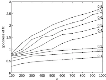
100 200 300 400 500 600 700 800 900 1000 0
0.5 1 1.5 2 2.5 3
0.1 0.2 0.3 0.4 0.5 0.6 0.7 0.8
n
goodness of fit
Fig. 2. Same as in Figure 1 but for the goodness of fit measure based
on RMSE of the estimatedφ(see text for details).
experiments is at least as relevant as the use of the common global MLE method. Usually for smallnand small1φwe do not detect nonstationarity, and the resulting estimate coin-cides with the global estimate. What we see in these cases in Fig. 1 is the effect of overestimating AICCAWSby usingk=4
instead of the correctk=2 if nonstationarity was not detected. This approach however does not demonstrate if the method does detect the presence of jumps in the parameters of the modeled series. Using our prior knowledge of the experi-mental design we define a second goodness of fit measure from the RMS error of the estimatedφ relative to the true one. For each run of AWS in m=1, ..., M with {n, 1φ}, RMSE{mn,1φ}, the root mean square error in φ of the
esti-mated model
n
ˆ
φ(t ),bσ2(t )
o
was calculated. A simple ap-proach to quantify the capability of the method to capture the sudden change inφfor a given{n, 1φ}, is to compare the RMSE{n,1φ} with1φ. The respective goodness of fit statistics is defined as
g{n,1φ}=
1φ
2RMSE{n,1φ} (18)
withg>1 being a critical value, implying that the procedure
has successfully separated the two segments with different correlation structures.
Figure 2 displays the family curve with estimated values ofQ0.95
RMSE{n,1φ} for different values of1φ. HereQ0RMSE.95 {n,1φ}
50 100 150 200 250 300 350 400 450 500 0
0.05 0.1 0.15 0.2 0.25 0.3
0
0.1 0.2
0.9
n
CI
0.95
Fig. 3. Double width of the 95% confidence interval (CI95%) for
the global maximum likelihood estimate ofφfor different values of
a time-series lengthnand with autocorrelation coefficientφ.
case of the global MLE (see Eq. 7 and Fig. 3). One should note, however, that this numerical experiment disregards the actual values ofφ1andφ2, whereas the width of the
confi-dence interval forφˆ varies substantially withφandn. Fig-ure 2 therefore provides the mean estimates of the goodness of fit as the whole range of possible (φ1,φ2) is considered.
7.2 Synthetic time-series
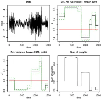
A simple synthetic series containingn=1500 data points is constructed by concatenation of segments of different lengths with locally constantφandσ2. The AWS results are shown in Fig. 4. The figure demonstrates the ability of the method to successfully localize discontinuities in the model parameters by a propagation of weights within homogeneous regions. Note that despite some discrepancy between the true (dotted lines) and estimated (solid lines) values ofφandσ2, a good agreement is generally reached.
Figure 5 shows the second example where the method is applied to a series of lengthn=1000 withσ2=1 andφ chang-ing linearly from –0.99 to 0.99. Forhmax=n the method
yields piecewise constant estimates ofφ andσ2, in accor-dance with the structural assumption of local stationarity. Note that the magnitudes of jumps inφ and the correspon-dent segment lengths are close to the minimal detectable ones for the considered1φn , as Fig. 2 shows.
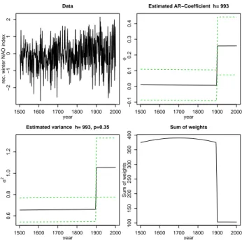
7.3 Reconstructed winter NAO index
Figure 6 shows the AWS analysis of the winter (December through March) North Atlantic Oscillation (NAO) index re-construction for the period 1500–1997 published in (Luter-bacher et al., 2002) (the series is available in the World Data Center for Paleoclimatology at http://www.ncdc.noaa.
0 500 1000 1500
−4
−2
0
2
4
time
data
Data
0 500 1000 1500
−0.4
0.0
0.4
0.8
time
φ
Est. AR−Coefficient hmax= 2000
0 500 1000 1500
0.0
1.0
2.0
3.0
time
σ
2
Est. variance hmax= 2000, p=0.0
0 500 1000 1500
100
200
300
400
time
Sum of weights
Sum of weights
Fig. 4. Synthetic time-series with piecewise constantφandσ2(top left); AWS estimates of the autocorrelation coefficient (solid lines, top right) and variance (solid lines, bottom left); sum of weights, N (t )(bottom right). Dotted lines show the true values of φand
σ2used when modeling the time-series. Dashed lines outline the
confidence limits for the estimates ofφandσ2. A p-value of the
Shapiro-Wilk test for normality of the residuals is shown above the left bottom panel.
gov/paleo/wdc-paleo.html). The NAO is the dominant pat-tern of atmospheric circulation variability over the North At-lantic basin, having large impacts on weather and climate in the North Atlantic region and surrounding continents. The NAO index, which is defined as the time-averaged difference of sea level pressure (SLP) between Iceland and the Azores, reflects the strength of the westerly across the Atlantic basin into Europe (note that there also exist alternative definitions of the NAO index, see for example van Loon and Rogers, 1978).
Luterbacher et al. (2002) provide a proxy- and early instru-mental data based reconstruction of the seasonal and monthly NAO indices. We used winter means for the earlier part of the record for 1500–1668 and derived mean December through March indices from the respective monthly means for the rest of the period.
0 200 400 600 800 1000
−10
−5
0
5
10
time
data
Data
0 200 400 600 800 1000
−1.0
−0.5
0.0
0.5
1.0
time
φ
Estimated AR−Coefficient h= 1940
0 200 400 600 800 1000
0.8
1.0
1.2
1.4
time
σ
2
Estimated variance h= 1940, p=0.67
0 200 400 600 800 1000
150
200
250
time
Sum of weights
Sum of weights
Fig. 5. Same as in Fig. 4 but for synthetic time-series withσ2=1
andφchanging linearly from –0.99 to 0.99.
instrumental station-based winter-mean NAO SLP index for the shorter period of 1864–1996. Weak positiveφin the 20th century reflects a tendency for the NAO to have a slightly “red” spectrum, what can be attributed to the enhanced vari-ability at decadal scale in the 20th century (Hurrell and van Loon, 1997). Note that the change inφˆ is accompanied by the increase in the estimated variance, which can also be as-cribed to strengthening of the decadal variability in the NAO. A simple AR(1) model fitted to the data, despite being ade-quate for the analyzed time-series on average, is not capable of capturing the quasi-oscillatory behavior in the data. Yet it may provide an indication that the character of the depen-dence in the analyzed series has changed.
7.4 Reconstructed boreal winterN ieno−3 index
The next example shows the application of AWS to the re-constructed boreal winterN ieno−3 index (Mann et al., 2000) covering the period 1650–1980 (data from http://www.ncdc. noaa.gov/paleo/wdc-paleo.html). The N ieno−3 index is based on the eastern tropical Pacific sea surface tempera-tures and serves as one of the indicators of the global El Nino/Southern Oscillation (ENSO) variability. Positive and negative values of the N ieno− 3 index indicate El Ni˜no (warm) and La Ni˜na (cold) episodes, respectively.
Figure 7 reveals a substantial decrease inφˆ between the two intervals of not rejected local stationarity with respect to the AR(1) model fitted to the reconstructedN ieno−3 index. The change most likely occurred around 1800, and is accom-panied by a rise in the estimated value ofσ2. We suggest
1500 1600 1700 1800 1900 2000
−2
−1
0
1
2
year
rec. winter NAO index
Data
1500 1600 1700 1800 1900 2000
−0.1
0.0
0.1
0.2
0.3
0.4
year
φ
Estimated AR−Coefficient h= 993
1500 1600 1700 1800 1900 2000
0.6
0.8
1.0
1.2
year
σ
2
Estimated variance h= 993, p=0.35
1500 1600 1700 1800 1900 2000
100
150
200
250
300
350
400
year
Sum of weights
Sum of weights
Fig. 6. Reconstructed winter NAO index (top left); AWS estimates
of the autocorrelation coefficient (top right) and variance (bottom
left); sum of weights,N (t )(bottom right). Dashed lines outline the
confidence limits for the estimates ofφandσ2.
1650 1750 1850 1950
−1.0
−0.5
0.0
0.5
1.0
year
rec. winter Nino−3 index
Data
1650 1750 1850 1950
0.0
0.1
0.2
0.3
0.4
0.5
0.6
0.7
year
φ
Estimated AR−Coefficient h= 635
1650 1750 1850 1950
0.05
0.10
0.15
0.20
0.25
year
σ
2
Estimated variance h= 635, p=0.05
1650 1750 1850 1950
140
150
160
170
180
year
Sum of weights
Sum of weights
Fig. 7. Same as in Fig. 6 but for the reconstructed boreal winter
60000 40000 20000 0
−1
0
1
2
year B.P.
GRIP d18O anomaly
Data
60000 40000 20000 0
0.7
0.8
0.9
1.0
year B.P.
φ
Estimated AR−Coefficient h= 1240
60000 40000 20000 0
0.00
0.10
0.20
0.30
year B.P.
σ
2
Estimated variance h= 1240, p=0.0
60000 40000 20000 0
100
150
200
250
300
350
400
year B.P.
Sum of weights
Sum of weights
Fig. 8. Same as in Fig. 6 but for the resampled GRIPδ18Oseries.
that this provides an indication of a change in the character of the dependence in the correlation structure of the analyzed series. During the first half of the considered period the re-constructedN ieno−3 index exhibits a negative trend which levels out in the early 19th century. We note that the presence of this long-term trend component is not consistent with the simple model fitted to the data and partly accounts for the elevated values ofφˆbefore 1800.
The tendency towards decreased ENSO variability before 1850 has been argued for in previous proxy-based ENSO studies (see for example Stahle and Cleaveland, 1993). Mann et al. (2000), in turn, came to a similar conclusion having ap-plied the evolutive spectral analysis to the sameN ieno−3 index reconstruction. The analysis revealed an enhanced in-terannual variability after the mid 19th century, which also agrees well with our estimates.
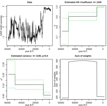
7.5 GRIP oxygen isotope series
In the last example we apply the AWS technique to GRIP (Greenland Ice Core Project) ice coreδ18Oseries (Johnsen, 1999) which serves, to a large extent, as an indicator of past temperature changes at the core site. The analyzed part of the record covers some 60 000 years and is originally un-evenly sampled in time. We resampled the time-series using 100 year bins and calculated the normalized anomalies. The time increment of 100 years for the procedure is chosen so that at least one data point falls within the resampling inter-val in the oldest part of the series under consideration. In the upper part of the core the data density is higher, varying
be-tween 25 data points per bin in the 20th century to 5 at the termination of the last glacial period around 12 000 years BP. Figure 8 suggest an increase in the serial autocorrelation coefficient GRIP δ18O with the onset of the Holocene ac-companied by a decrease in the estimated variance. This re-sult represents a combined effect of actual climate variabil-ity and a bias introduced in the series by data interpolation. On one hand, the Holocene is characterized by a more sta-ble climate compared with the last glacial period punctuated by a series of abrupt warmings – the so-called Dansgaard-Oeschger oscillations (Dansgaard et al., 1993). On the other hand the resampling is known to alter the series autocovari-ance structure by bringing additional dependence to the data (Schulz and Stattegger, 1997). The latter effect will natu-rally be more pronounced in the uppermost part of the ice core series where the sampling density in the time domain is higher and each point in the resampled series is an average over a number of original observations. As a reference we es-timated the autocorrelation using the RedFit package (Schulz and Mudelsee, 2002) which fits the AR(1) model directly to an unevenly spaced time series. The separate analysis of the Holocene and glacial parts of the original GRIPδ18Oseries yields the values ofφof 0.01 and 0.87, respectively, which are below the corresponding AWS estimates.
8 Conclusions
We presented a method which employs the idea of structural adaptation for fitting an AR(1) model to a time-series. The approach utilizes an assumption of a local stationary AR pro-cess. This is used to simultaneously generate local weighting schemes, i.e. a local model, and to estimate the parameters of the AR(1) model as functions of time by weighted maximum likelihood. The proposed procedure leads, for a large maxi-mum bandwidth (hmax) to a local constant approximation of
these parameter functions. This seems appropriate if periods of local stationarity are separated by shorter periods of rapid change. The approach implicitly provides a test for global stationarity, i.e. leads to the global AR(1) model if stationar-ity cannot be rejected.
An implementation of the AWS method is available from the authors as a package (acoraws) for the R-Project for Sta-tistical Computing (R Development Core Team, 2005). Acknowledgements. The authors thank WIAS for hosting D.Divine. This study was financially supported by the Norwegian Research Council, projects 160008/v30 and 176872/v30.
Edited by: J. Kurths
References
Box, E., Jenkins, G., and Reinsel, G.: Time series analysis: Fore-casting and control, Prentice-Hall, Englewood Cliffs, 1994. Brockwell, P. and Davis, R.: Time series: theory and methods,
Springer, New York, 1998.
Burnham, K. and Anderson, D.: Model selection and multimodel inference: a practical-theoretic approach, Springer, 2002. Chen, C., H/”ardle, W., and Unwin, A.: Handbook of Data
Visual-ization, Springer, 2008.
Dansgaard, W., Johnsen, S., Clausen, H., Dahl-Jensen, D., Gunde-strup, N., Hammer, C.U.and Hvidberg, C., Steffensen, J., Svein-bjornsdottir, A., Jouzel, J., and Bond, G.: Evidence for general instability of past climate from a 250-kyr ice-core record, Nature, 364, 218–220, doi:10.1038/364218a0, 1993.
Hasselmann, K.: Stochastic climate models: Part I. Theory, Tellus, 28(6), 473-485, 1976.
Hurrell, J. and van Loon, H.: Decadal variations in climate asso-ciated with the North Atlantic Oscillation, Climate Change, 36, 301–326, 1997.
Johnsen, S.: GRIP Oxygen Isotopes, PANGAEA, doi:10.1594/ PANGAEA.55091, 1999.
Luterbacher, J., Xoplaki, E., Dietrich, D., Jones, P., Davies, T., Por-tis, D., Gonzalez-Rouco, J., von Storch, H., Gyalistras, D., Casty, C., and Wanner, H.: Extending North Atlantic Oscillation Recon-structions Back to 1500, Atmos. Sci. Lett., 2, 114–124, 2002.
Mann, M., Bradley, R., and Hughes, M.: Long-term variability in the El Nino Southern Oscillation and associated teleconnections, in: El Nino and the Southern Oscillation: Multiscale Variabil-ity and its Impacts on Natural Ecosystems and Society, edited by Diaz, H. and Markgraf, V., Cambridge University Press, Cam-bridge, UK, 2000.
Polzehl, J. and Spokoiny, V.: Adaptive weights smoothing with ap-plication to image restoration, Journal of the Royal Statistical Society, 62(B), 335–354, 2000.
Polzehl, J. and Spokoiny, V.: Local likelihood modeling by adaptive weights smoothing, Preprint 787, WIAS, 2002.
Polzehl, J. and Spokoiny, V.: Propagation-separation approach for local likelihood estimation, Probab. Theory Related Fields, 135, 335–362, 2006.
R Development Core Team: R: A Language and Environment for Statistical Computing, Tech. Rep. ISBN 3-900051-07-0, R Foun-dation for Statistical Computing, Vienna, Austria, 2005. Schulz, M. and Mudelsee, M.: REDFIT: estimating red-noise
spec-tra directly from unevenly spaced paleoclimatic time series, Computers&Geosciences, 28, 421–426, 2002.
Schulz, M. and Stattegger, K.: SPECTRUM: spectral
analy-sis of unevenly spaced paleoclimatic time series, Comput-ers&Geosciences, 23, 929–945, 1997.