www.atmos-chem-phys.org/acp/2/387/
Chemistry
and Physics
On the use of ATSR fire count data to estimate the seasonal and
interannual variability of vegetation fire emissions
M. G. Schultz
Max Planck Institute for Meteorology, Hamburg, Germany
Received: 19 June 2002 – Published in Atmos. Chem. Phys. Discuss.: 12 August 2002 Revised: 23 October 2002 – Accepted: 18 November 2002 – Published: 28 November 2002
Abstract. Biomass burning has long been recognised as an important source of trace gases and aerosols in the atmo-sphere. The burning of vegetation has a repeating seasonal pattern, but the intensity of burning and the exact localisa-tion of fires vary considerably from year to year. Recent studies have demonstrated the high interannual variability of the emissions that are associated with biomass burning. In this paper I present a methodology using active fire counts from the Along-Track Scanning Radiometer (ATSR) sensor on board the ERS-2 satellite to estimate the seasonal and in-terannual variability of global biomass burning emissions in the time period 1996–2000. From the ATSR data, I compute relative scaling factors of burning intensity for each month, which are then applied to a standard inventory for carbon monoxide emissions from biomass burning. The new, time-resolved inventory is evaluated using the few existing multi-year burned area observations on continental scales.
1 Introduction
Emissions of greenhouse gases and pollutant species into the atmosphere have risen dramatically over the past century and have begun to exert a globally noticeable influence on the Earth’s climate and the welfare of it’s population (Houghton et al., 2001). Because of the spatial inhomogeneity and tem-poral variability of the emission sources and the atmospheric transport patterns, comprehensive three-dimensional models describing the physics and chemistry of the atmosphere are necessary in order to investigate the impact of these emis-sions on the global and regional scale. Several such mod-els have been developed over the past decade (c.f. Kasib-hatla et al., 1991; M¨uller and Brasseur, 1995; Atherton et al., 1996; Brasseur et al., 1998; Hauglustaine et al., 1998; Wang et al., 1998; Bey et al., 2001, Horowitz et al., submitted to Correspondence to:M. G. Schultz ([email protected])
J. Geophys. Res. 2002), and they are now beginning to be employed for decadal variability studies (e.g. Karlsdottir et al., 2000). Furthermore, such models have recently been put to use for forecasting atmospheric species concentrations in a number of large-scale airborne field experiments (c.f. Lawrence et al., 2002).
In order to achieve a realistic description of the atmo-spheric composition and for the comparison of model sim-ulations with observations, one has to take into account the variability in transport, UV radiation, and emissions of key trace gases and precursor species. The first is readily ac-complished through the use of assimilated meteorological fields provided by the large weather forecasting centers, e.g. ECMWF in Europe, or NCEP and NASA-DAO in the US. Interannual changes in tropospheric UV radiation can be ac-counted for by assimilating stratospheric ozone concentra-tions into the model. The model sensitivity towards strato-spheric ozone change has been assessed for example by Deleeuw and Leyssius (1991) and Fuglestvedt et al. (1994).
vari-388 M. G. Schultz: Variability of vegetation fire emissions
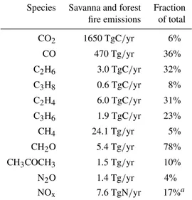
Table 1. Global annual emissions from savanna and forest fires and percent of total emissions for various species. Vegetation fire emission estimates from Hao and Liu (1994), M¨uller and Brasseur (1995), and Ward (1990), other emissions from Olivier et al. (1996) and M¨uller and Brasseur (1995) (details in Horowitz et al., submit-ted to J. Geophys. Res., 2002)
Species Savanna and forest Fraction
fire emissions of total
CO2 1650 TgC/yr 6%
CO 470 Tg/yr 36%
C2H6 3.0 TgC/yr 32%
C3H8 0.6 TgC/yr 8%
C2H4 6.0 TgC/yr 31%
C3H6 1.9 TgC/yr 23%
CH4 24.1 Tg/yr 5%
CH2O 5.4 Tg/yr 78%
CH3COCH3 1.5 Tg/yr 10%
N2O 1.4 Tg/yr 4%
NOx 7.6 TgN/yr 17%a
aTotal NO
xemissions include 4 TgN from lightning
ability of fire emissions on the global scale so far, is that of Duncan et al. (J. Geophys. Res., in press 2002), who use the Total Ozone Mapping Spectrometer (TOMS) aerosol index as a proxy for the emission flux.
It has long been recognised that biomass burning consti-tutes a major source term for a variety of pollution and ozone precursor species (e.g. Table 1), especially in the tropical lat-itudes and in the southern hemisphere, where emissions from fossil fuel combustion are relatively low. Vegetation burns for a variety of reasons, but fires are mostly of human origin with less than 20% being ignited by lightning strokes (c.f. Goldammer, 1990; Levine, 1996). Vegetation fires occur on different spatial scales and last from hours to weeks. For the purpose of this study the term biomass burning is restricted to open fires in the savanna and in tropical, temperate, and bo-real forests. Emissions from agricultural waste burning and fuelwood burning also add up to a large contribution to the global source of atmospheric pollutants, but they require a different treatment and are not discussed in this paper.
In order to estimate emissions from vegetation fires, one needs to know the amount of fuel that is available for burning and the percentage of fuel that is actually burned over a spe-cific time period. The amount of fuel that is burned in a given region and the fraction of fuel burned depend on a number of factors, such as the vegetation density, fuel composition and dryness, and meteorological parameters like wind speed, humidity, and temperature (c.f. Goldammer, 1990; Levine, 1996). For practical purposes, the emissions of other trace
gases and aerosol are typically scaled to the amount of CO2
released, although these emission ratios can vary depending on the type of combustion (e.g. flaming vs. smoldering fires, Andreae and Merlet, 2001). All of these parameters exhibit a great temporal and spatial variability, which has not been included in the global model inventories up to the present. Existing emission inventories (e.g. Hao and Liu, 1994) have been compiled using a variety of data from national reports (e.g. Goldammer, 1999) and a statistical approach in order to arrive at a globally consistent picture. The uncertainties of these inventories are considerable, and they are difficult to evaluate because of the seasonal and interannual variability of these emissions.
This paper presents a simple method to introduce the sea-sonal and interannual variability of biomass burning emis-sions into global emission inventories for atmospheric trace gases and aerosol. Monthly composites of active fires de-tected from space are used as a proxy for the relative strength of the biomass burning source in a model grid box. Cur-rently, this method is limited to the time period August 1996– December 2000, because of the availability of a consistent data set of global fire count data. However, with the suc-cessful launch of Envisat and the current push towards op-erational environmental prediction systems, it is likely that such data sets will become routinely available in the future. The 4-year inventory resulting from this study is evaluated by comparing its variability with literature estimates for specific regions.
2 Method
The compilation of a global inventory of biomass burning emissions is a labor-intensive and tedious task, requiring a lot of detailed knowledge about agricultural and landuse prac-tices, vegetation properties, and climatological conditions in individual countries and regions. Due to the sparsity of such information, the existing global inventories have to rely on statistical assumptions, which obviously prevent their use-fulness for assessing the interannual variability of fire emis-sions. Only few attempts have been made to assess the vari-ability of biomass burning on the continental scale (Barbosa et al., 1999b; Amiro et al., 2001; Wotawa et al., 2001).
Fig. 1. Areas with hot pixels in the ATSR world fire atlas, which are unlikely caused by vegetation burning. All 1◦×1◦grid boxes where
more than 3 active fires occur over 7 months each year are marked with a redx.
(Horowitz et al., submitted to J. Geophys. Res., 2002), which includes the inventories from Hao and Liu (1994) and Ward (1990) for tropical savanna and forest fires, respectively, and from M¨uller and Brasseur (1995) for temperate and boreal forest fires. The original 5◦×5◦inventory has been inter-polated onto a 1◦×1◦grid, and a land-sea mask has been applied in order to constrain emission fluxes to the land sur-face and to better localise the emission sources in individual years. Emission estimates for species other than CO2are
de-rived by calculating emission ratios from the emission factors given in Andreae and Merlet (2001).
Because there is no longer-term global data set of burned areas available at present, monthly composites of active fire observations from the ATSR sensor on board the ERS-2 satellite (Arino and Melinotte, 1998) are used as a surrogate (“world fire atlas” http://shark1.esrin.esa.it/ionia/ FIRE/). This data set is the only one with global coverage that is available for a reasonably long time period.
For the ATSR fire product, only nighttime observations are used, and a threshold of 312 K (algorithm 1) or 308 K (algo-rithm 2) is applied to the radiance of the 3.7µm channel in order to detect fires. The resolution of the ATSR sensor is 1×1 km2, which allows for detection of a 600 K hot spot of 0.1 ha or an 800 K hot spot of 0.01 ha (Arino and Melinotte, 1998). The sensor achieves complete global coverage every three days. Compared to daytime observations from the
Ad-vanced Very High Resolution Radiometer (AVHRR) (Bar-bosa et al., 1999a), the number of fires detected from the ATSR nighttime scans is considerably smaller. However, many of the fires detected during daytime are relatively small controlled burns, which generally attribute little to the large-scale regional burned area. The validity of this assumption is discussed in Sect. 3.
The ATSR data set contains a number of events from heat sources other than vegetation fires. These have been re-moved from the analysis based on the criterion that no grid box should contain more than 3 active fires for more than 7 months per year. This criterion is based on the presump-tion that true fire activity shows a distinct seasonality and usually ceases during winter or during the wet season. Visual inspection of the grid boxes that are removed from the analy-sis shows that they are predominantly located in areas where oil and gas flaring is known to occur, i.e. Northern Siberia, the Persian Gulf region, Mediterranean North Africa, etc. (Fig. 1). A few falsely detected fires are also seen in the Sa-hara region.
390 M. G. Schultz: Variability of vegetation fire emissions
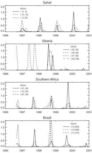
Fig. 2.Time series of the normalised monthly fire occurence in se-lected grid boxes. The fire frequency has been derived by sampling
ATSR nighttime active fire observations into 1◦×1◦grid boxes.
fires throughout the 5-year period and ocean grid boxes are marked with a 0 value.
Figure 2 shows the resulting scale factors for a few se-lected grid boxes as a function of time. The seasonality generally follows the expected behaviour with most intense burning in the dry seasons, i.e. December/January for the Sa-hel, July/August for the northern hemisphere boreal forests, and September/October for southern hemispheric Africa and South America. There is considerable variability from year to year for some grid boxes, whereas others (notably in the Sahel) exhibit a relatively periodic pattern. Because of the long fire return interval in boreal regions (c.f. Thonicke et al., 2001), some of the grid boxes in Fig. 2 show fire activity only during one of the 5 years (e.g. 83◦E, 49◦N in 1997, and 50◦E, 50◦N in 1998). It should be emphasized, that Fig. 2 does not contain information about the differences between grid boxes, but only shows the time series of fire occurences within individual boxes.
The final step in deriving biomass burning emissions for individual years and months is multiplication of the scale factors with the “climatological” annual biomass burning
emissions from the MOZART2 inventory. The result is a monthly resolved, global gridded inventory of savanna and forest burning emissions for the time period August 1996 – December 2000.
Some of the grid boxes do not exhibit any fire activity during the time period considered here, but they are associ-ated with non-zero emissions in the climatological inventory. Therefore, the average annual global total of the CO emis-sions from the new inventory is about 15% lower than the an-nual total of the original inventory of the MOZART2 model. While this is well within the uncertainty range for biomass burning emissions, I decided to apply a uniform scaling fac-tor of 1.2 to the new invenfac-tory in order to facilitate com-parison with previous model results and to be able to investi-gate the effects from the better localisation and timing of fires without changing the global “background” concentrations.
3 Results and evaluation
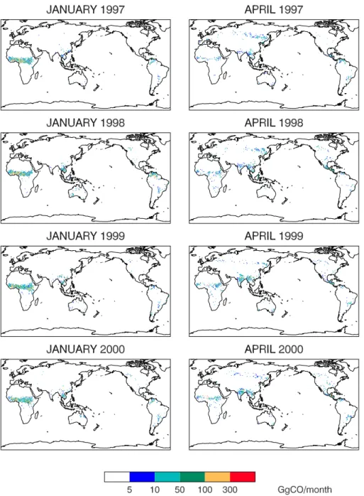
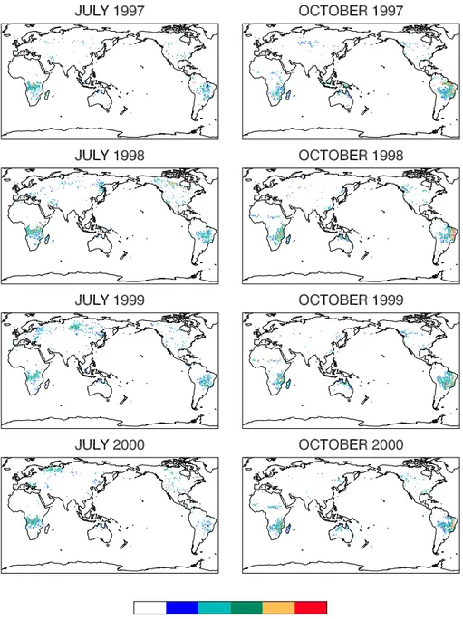
As an example for the final product, Fig. 3 shows the global biomass burning emission inventory for CO for the months of January, April, July, and October in the individual years from 1997 to 2000. One can clearly identify a number of outstanding events, such as the Indonesian forest fires in Oc-tober 1997, or the Canadian boreal fires in the summer of 1998. Significant interannual variability is seen in Southern Africa and South America during the fire season from July to October, as well as in northern India, South East Asia, and Central America in April.
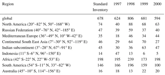
Table 2 lists the cumulated annual CO emissions from biomass burning for various regions and compares them with the base emission inventory. The largest year-to-year vari-ability can be seen in Indonesia, where the extreme fires in 1997 led to a factor of 3 increase in the emissions of CO. Africa and South America are estimated to have the largest emissions from fires and show the lowest interannual vari-ability (20% and 30%, respectively). According to the scal-ing method, 1998 was the year with the largest biomass burn-ing emissions in the four-year period. Globally, the release of CO is estimated to be 20% higher in 1998 than on average, and it is highest in all the regions listed in Table 2, except for continental South East Asia, the Indian subcontinent, and In-donesia. This result is in qualitative agreement with the study of Duncan et al. (J. Geophys. Res., in press 2002), who use a more elaborate method involving different satellite prod-ucts. The reasons of this significantly increased fire activity are not clear yet, but several news reports indicate that 1998 has been an exceptionally dry year. From the ATSR data set, it becomes clear that enhanced fire frequency was not lim-ited to one region and season, but affected several areas of the world at different times.
Fig. 3. Monthly global 1◦×1◦emissions of carbon monoxide from forest and savanna burning for January and April 1997–2000 after applying the scale factors derived from the ATSR active fire observations (unit: GgCO/month)
contains information about the variability and the timing specifically of the larger fires, which very likely constitute the majority of the burnt area, at least in boreal and tem-perate forests (Stocks, 1991). Assuming that the amount of biomass that is available for burning does not vary too much from year to year and within a given geographic region, the variability in the number of nighttime fires should therefore be a good proxy for the variability in burnt area, and the vari-ability in burnt area should provide a reasonable estimate of the variability in the emissions.
The year-to-year changes of the burned area in North
392 M. G. Schultz: Variability of vegetation fire emissions
Fig. 4.Dto. for July and October
For savanna fires, the relationship between fire counts and emissions is not as straight forward, because of the large frac-tion of small controlled daytime burns in these regions. Hely et al. (J. Geophys. Res., in press, 2002) estimate that approx-imately 50% of the burnt area in southern Africa during the dry season is produced from fires smaller than 2 km2. Never-theless, even in these regions a correlation may exist between the relative frequency of active fire observations and vegeta-tion fire emissions, because – regardless of the scale – the intensity and spread of fires will depend on the same param-eters (humidity, temperature, wind speed, etc.). Therefore, in an integral sense, the relative change in the number of large
intensive fires in a grid box should provide a first order ap-proximation for the variability of the trace gas emissions in that region.
Table 2.Regional totals of biomass burning emissions estimated from the ATSR scale factor approach (in TgCO/yr)
Region Standard 1997 1998 1999 2000
Inventory
global 678 624 806 681 594
North America (20◦–82◦N, 50◦–168◦W) 74 40 88 68 63
Russian Federation (40◦–76◦N, 42◦–185◦E) 47 39 59 37 40
Mediterranean Europe (36◦–49◦N, 10◦W–42◦E) 35 18 46 34 44
Continental South East Asia (7◦–30◦N, 92◦–119◦E) 46 29 64 70 27
Indian subcontinent (3◦–28◦N, 67◦–91◦E) 45 30 36 63 47
Indonesia (11◦S–6◦N, 96◦–150◦E) 14 47 13 6 5
Africa (42◦S–22◦N, 22◦W–53◦E) 198 195 239 173 198
South America (54◦S–11◦N, 33◦–82◦W) 146 166 196 159 100
Australia (45◦–10◦S, 114◦–156◦E) 16 18 13 22 20
area, which naturally results in a range for the emission es-timates as well. For the period November 1985–October 1991 they derive CO emissions of 40±11Tg/yr (low es-timate) to 152±41Tg/yr (high estimate). In absolute values, these estimates are lower by a factor of 1.3–5 compared to those from the standard inventory used in this study. This is due to the lower burned area estimates by B99 compared to Hao and Liu (1994). B99 also use somewhat different emis-sion factors (230 g/kg and 68 g/kg for tropical forests and savanna, respectively compared to 104 g/kg and 65 g/kg from Andreae and Merlet (2001)). The percent variability (1σ/mean×100) of the B99 emission estimates is 27% for both the low and high estimates. This is almost twice as high as the variability of 14% that can be derived from Table 2. If the scaled emissions are analysed for “fire years” instead of calendar years, the interannual variability is slightly in-creased to 17%. Broken down by latitude, the variability in southern hemispheric Africa, where 43% of the emissions are located, amounts to 25% in the scaled inventory, whereas northern hemispheric Africa only varies by 13% between the years.
The different variability estimates might in part be ex-plained by variations in fuel load and burning efficiency, which have been taken into account by B99 using a cor-relation with the normalised differential vegetation index (NDVI) as a proxy for the biomass density and an inverse correlation with the relative greeness index (RGI) for esti-mating the burning efficiency. Another important aspect is the subgrid-scale variability of vegetation types and their dif-ferent burning behaviour. Since the scaling approach starts from a gridded emission inventory, it necessarily assumes average vegetation properties. B99 provide annual burned area estimates for 16 individual vegetation classes. Interan-nual variability of burned area ranges from less than 10% for some classes to more than 50% for other classes. Averaged
1990 1992 1994 1996 1998 2000 Year
0 20 40 60 80
CO emissions [Tg/yr]
0 2000 4000 6000 8000
Burnt area [1000 ha]
North America Former USSR
Fig. 5.Comparison of the variability of CO emissions from biomass burning (this study, filled symbols) with estimates of burned area for North America and the Russian Federation (Wotawa et al., 2001, open symbols).
over all vegetation classes, the variations in the burned area of B99 account for 95% of the variability in the CO emis-sions.
emis-394 M. G. Schultz: Variability of vegetation fire emissions sions and provide a better measure of the variability if they
are augmented by information on the vegetation type and fuel load on a high resolution.
4 Conclusions
The use of ATSR fire count data to derive scaling factors for a global biomass burning emission inventory is a simple ap-proach that allows for a more realistic description of partic-ular large-scale fire situations compared to the present use of average emissions in global chemistry transport model-ing. It has been demonstrated that the normalized scaling method qualitatively reproduces outstanding fire events. The algorithm produces an interannual variability that is similar to the variability observed in burned area statistics for some regions (e.g. North America and Southern Africa), but only about half as large in other regions (e.g. Russian Federation and Sahel). However, these comparisons remain somewhat qualitative, because there is no direct quantitative relation be-tween the burned area and the trace gas and aerosol emissions from fires.
Preliminary model results indicate that the impact of us-ing these more localised and intense emissions on the CO concentration can easily reach 30% in the free troposphere downwind of emission regions. A more detailed analysis of the model results will be subject of a different paper.
With over four years of sampling, the ATSR data set is beginning to become statistically robust, and there is rea-son to believe that a similar and consistent product will also be available from the Advanced Along-Track Scanning Ra-diometer (AATSR) on the recently launched Envisat. New satellite products giving estimates of the burned area, such as GLOBSCAR, GBA 2000 (Gr´egoire et al., 2002) or the Vegetation Cover Change product from the Moderate Res-olution Imaging Spectroradiometer (MODIS) will be aug-mented with high-resolution vegetation data. This will allow for a more quantitative estimate of emissions in individual years by allowing to reprocess the inventory from scratch for each year instead of scaling an existing inventory. For multi-year simulations of the past, the fire count approach should be considered as an interim solution until such more sophis-ticated products become available.
A new and emerging application of global chemistry trans-port models is the prediction of pollutant concentrations (“chemical weather”) to provide boundary conditions for re-gional forecast models or to support large-scale field experi-ments. Because of the simplicity of the technique, the active fire scaling approach appears well suited for quasi-realtime emission estimates as they will be necessary for such endeav-ours. However, this would require a near real-time opera-tional active fire satellite data product, which is currently not available.
Acknowledgements. The author would like to thank O. Arino and M. Simon (European Space Agency) for providing the ATSR fire
count data and detailed information on the algorithms and process-ing chain of these data. W. M. Hao, J. A. Logan, and J. Goldammer deserve a lot of credit for helpful discussions on the subject, and C. Granier, B. Langmann, and J. H¨olzemann for reviewing draft ver-sions of this manuscript.
References
Atherton, C., Sillman, S., and Walton, J.: Three-dimensional global modeling studies of the transport and photochemistry over the north atlantic ocean, J. Geophys. Res.-Atmos., 101, 29 289– 29 304, 1996.
Amiro, B., Todd, J., Wotton, B., Logan, K., Flannigan, M., Stocks, B., Mason, J., Martell, D., and Hirsch, K.: Direct carbon emis-sions from canadian forest fires, 1959–1999, Can. J. For. Res.-Rev. Can. Rech. For., 31, 512–525, 2001.
Andreae, M. and Merlet, P.: Emission of trace gases and aerosols from biomass burning, Glob. Biogeochem. Cycle, 15, 955–966, 2001.
Arino, O. and Melinotte, J.: The 1993 africa fire map, Int. J. Remote Sens., 19, 2019–2023, 1998.
Barbosa, P., Gregoire, J., and Pereira, J.: An algorithm for extract-ing burned areas from time series of avhrr gac data applied at a continental scale, Remote Sens. Environ., 69, 253–263, 1999a. Barbosa, P. M., Stroppiana, D., Gr´egoire, J.-M., and Pereira, J.
M. C.: An assessment of vegetation fire in africa (1981–1991): Burned areas, burned biomass, and atmospheric emissions, Global Biogeochem. Cyc., 13, 933–950, 1999b.
Bey, I., Jacob, D., Yantosca, R., Logan, J., Field, B., Fiore, A., Li, Q., Liu, H., Mickley, L., and Schultz, M.: Global modeling of tropospheric chemistry with assimilated meteorology: Model de-scription and evaluation, J. Geophys. Res.-Atmos., 106, 23 073– 23 095, 2001.
Brasseur, G., Hauglustaine, D., Walters, S., Rasch, P., Muller, J., Granier, C., and Tie, X.: Mozart, a global chemical transport model for ozone and related chemical tracers 1. model descrip-tion, J. Geophys. Res.-Atmos., 103, 28 265–28 289, 1998. Cooke, W. F., Koffi, B., and Gr´egoire, J.-M.: Seasonality of
vegeta-tion fires in Africa from remote sensing data and applicavegeta-tion to a global chemistry model, J. Geophys. Res.-Atmos., 101, 21 051– 21 066, 1996.
Deleeuw, F. and Leyssius, H.: Sensitivity of oxidant concentrations on changes in UV-radiation and temperature, Atmos. Environ. Part A-General Topics, 25, 1025–1032, 1991.
Dwyer, E. J., Pereira, J. M. C., Gr´egoire, J.-M., and DaCamera, C. C.: Characterization of the spatio-temporal patterns of global fire activity using satellite imagery for the period April 1992 to March 1993, J. Biogeography, 1, 57–69, 1999.
Fuglestvedt, J., Jonson, J., and Isaksen, I.: Effects of reductions in stratospheric ozone on tropospheric chemistry through changes in photolysis rates, Tellus Ser. B-Chem. Phys. Meteorol., 46, 172–192, 1994.
Goldammer, J.: International forest fire news, Tech. Rep. 21, UN-ECE and FAO, 1999.
Goldammer, J. G.: (Ed) Fire in the Tropical Biota, vol. 84 of Eco-logical Studies, Springer, 1990.
Hao, W. and Liu, M.: Spatial and temporal distribution of tropical biomass burning, Glob. Biogeochem. Cycle, 8, 495–503, 1994. Hauglustaine, D., Brasseur, G., Walters, S., Rasch, P., Muller, J.,
Emmons, L., and Carroll, C.: Mozart, a global chemical transport model for ozone and related chemical tracers 2. model results and evaluation, J. Geophys. Res.-Atmos., 103, 28 291–28 335, 1998. Houghton, J., Ding, Y., Griggs, D., Noguer, M., van der Linden, P., Dai, X., Maskell, K., and Johnson, C.: (Eds) Climate Change 2001: The scientific basis, Contribution of Working Group I to the Third Assessment Report of the Intergovernmental Panel on Climate Change, Cambridge University Press, 2001.
Karlsdottir, S., Isaksen, I., Myhre, G., and Berntsen, T.: Trend analysis of O-3 and CO in the period 1980–1996: A three-dimensional model study, J. Geophys. Res.-Atmos., 105, 28 907– 28 933, 2000.
Kasibhatla, P., Levy, H., Moxim, W., and Chameides, W.: The rela-tive impact of stratospheric photochemical production on tropo-spheric noy levels – a model study, J. Geophys. Res.-Atmos., 96, 18 631–18 646, 1991.
Lavou´e, D., Liousse, C., Cachier, H., Stocks, B., and Goldammer, J.: Modeling of carbonaceous particles emitted by boreal and temperate wildfires at northern latitudes, J. Geophys. Res.-Atmos., 105, 26 871–26 890, 2000.
Lawrence, M., Rasch, P. J., von Kuhlmann, R., Williams, J., Fis-cher, H., de Reus, M., Lelieveld, J., Crutzen, P. J., Schultz, M. G., Stier, P., Huntrieser, H., Heland, J., Stohl, A., Forster, C., Elbern, H., Jakobs, H., and Dickerson, R. R.: Global chemical weather forecasts for field campaign planning: predictions and observa-tions of large-scale features during MINOS, CONTRACE, and INDOEX, Atmos. Chem. Phys. Discuss., 2, 1545–1597, 2002. Levine, J. S.: (Ed) Biomass Burning and Global Change, vol. 1, The
MIT Press, Massachusetts Institute for Technology, 1996.
M¨uller, J. and Brasseur, G.: Images – a 3-dimensional chemical-transport model of the global troposphere, J. Geophys. Res.-Atmos., 100, 16 445–16 490, 1995.
Olivier, J., Bouwman, A., van der Maas, C., Berdowski, J., Veldt, C., Bloos, J., Visschedijk, A., Zandveld, P., and Haverlag, J.: Description of EDGAR Version 2.0: A set of global emission inventories of greenhouse gases and ozone-depleting substances for all anthropogenic and most natural sources on a per country
basis and on 1×1 grid, Tech. Rep. 771060 002, RIVM,
TNO-MEP, 1996.
Stocks, B.: The Extent and Impact of Forest Fires in Northern Cir-cumpolar Countries, MIT Press, Cambridge, London, pp. 197– 202, 1991.
Thonicke, K., Venevsky, S., Stitch, S., and Cramer, W.: The role of fire disturbance for global vegetation dynamics: Coupling fire into a global vegetation model, Global Ecol. Biogeogr., 10, 661– 677, 2001.
van Aardenne, J., Dentener, F., Olivier, J., Klein Goldewijk, C., and
Lelieveld, J.: A 1×1 resolution data set of historical
anthro-pogenic trace gas emissions for the period 1890–1990, Global Biogeochem. Cyc., 15, 909–928, 2001.
Wang, Y., Jacob, D., and Logan, J.: Global simulation of tropo-spheric o-3-nox-hydrocarbon chemistry 1. model formulation, J. Geophys. Res.-Atmos., 103, 10 713–10 725, 1998.
Ward, D. E.: Factors Influencing the Emissions of Gases and Partic-ulate Matter from Biomass Burning, vol. 84 of Ecological Stud-ies, chap. 18, pp. 418–425, Springer, 1990.