No 655 ISSN 0104-8910
The Effects of External and Internal Strikes
on Total Factor Productivity
Pedro C. Ferreira, Antonio Galvao, Samuel Pess ˆoa
Os artigos publicados são de inteira responsabilidade de seus autores. As opiniões
neles emitidas não exprimem, necessariamente, o ponto de vista da Fundação
The E¤ects of External and Internal Strikes on Total
Factor Productivity
Pedro C. Ferreira
yFGV - EPGE
Antonio Galvao
University of Illinois
Samuel Pessôa
FGV - EPGE
September 28, 2007
Abstract
This paper examines structural changes that occur in the total factor produc-tivity (TFP) within countries. It is possible that some episodes of high economic growth or economic decline are associated with permanent productivity shocks, therefore, this research has two objectives. The …rst one is to estimate the struc-tural changes present in TFP for a sample of 81 countries between 1950(60) and 2000. The second one is to identify, whenever possible, episodes in the political and economic history of these countries that may account for the structural breaks in question. The results suggest that about 85% of the TFP time-series present at least one structural break, moreover, at least half the structural changes can be at-tributed to internal factors, such as independence or a newly adopted constitution, and about 30% to external shocks, such as oil shock or shocks in international in-terest rates. The majority of the estimated breaks are downwards, indicating that after a break the TFP tends to decrease, implying that institutional rearrange-ments, external shocks, or internal shocks may be costly and from which it is very di¢cult to recover.
Keywords: total factor productivity, structural breaks
JEL Classi…cation: O47, O50.
The authors would like to express their appreciation to Derek Laing and Zhongjun Qu for helpful comments. All the remaining errors are ours. Ferreira would like to thank CNPq and Pronex for the …nancial support.
yFerreira and Pessoa: Fundação Getulio Vargas, Brazil. Emails: [email protected] and [email protected].
1
Introduction
One of the main characteristics of modern economies is the large di¤erences in per capita
income among countries. Explaining these di¤erences and their evolution over time is
an extremely important problem. In a seminal paper Mankiw, Romer, and Weil (1992)
investigate the capacity of Solow’s growth model to explain the levels of relative variations
in per capita income across countries and suggest that the di¤erences can be well described
using the augmented Solow model that accounts for accumulation of both physical and
human capital. Using structural breaks technique, Ben-David and Papell (1998) proposed
a test for determining the signi…cance and the timing of slowdowns in economic growth.
They were able to show evidence that most industrialized countries experienced postwar
growth slowdowns in the early 1970s, and that developing countries, in particular Latin
American countries, tended to experience even more severe slowdowns.
Economists have recognized, however, that total factor productivity (TFP) acts as a
determinant factor in the growth process. TFP is usually estimated as a residual using
the index number technique.1 This residual captures changes in the output that cannot
be explained by variations in the quantities of inputs, capital and labor. Intuitively,
the residual re‡ects an upward (or downward) shift in the production function. Many
factors can cause this shift, such as technological innovation, organizational and
institu-tional changes, demand ‡uctuations, changes in the factors composition, external shocks,
omitted variables and measurement errors.2
Hall and Jones (1999), Parente and Prescott (1999), Prescott (1998), Klenow and
Rodriguez-Claire (1997), among others, show that there is strong evidence that TFP
is considerably responsible for the di¤erences in per capita income across countries. A
substantial part of those di¤erences in output levels can only be partially explained by
1Di¤erent approaches were proposed by Lagos (2006), Parente and Prescott (1999), and Krusell and
Rios-Rull (1996). The …rst study proposes an aggregative model of TFP considering a frictional labor market where production units are subject to idiosyncratic shocks in which jobs are created and destroyed. Therefore, the level of TFP is explicitly shown to depend on the underlying distribution of shocks as well as on all the characteristics of the labor market as summarized by the job-destruction decision. The last two studies propose a theory to explain how institutional arrangements a¤ect TFP, introducing elements of strategic behavior in dynamic general equilibrium models. These studies ultimately try to explain why societies chose these institutions, in an explicit attempt to endogenize this choice.
di¤erences in physical capital and education, but the largest part of these di¤erences are
explained by the Solow residual, that is, the total factor productivity. Therefore, the
di¤erence in capital accumulation, productivity and consequently in output per worker
is the outcome of di¤erences in institutions and government policies of each individual
country. The institutions and public policies structure existent in each country are de…ned
by the authors as the social infrastructure. Thus, the result points to a strong correlation
between output per worker and the social infrastructure indicator, in such a way that
countries with public policies that are favorable to productive activities tend to produce
more output per worker.
More recently, Jones and Olken (2007) estimated structural breaks for income growth
rates and employed growth accounting technique to investigate what occurs during
var-ious transitions. Their analysis suggests that changes in the rate of factor accumulation
explain relatively little about the growth reversals. Instead, the growth reversals are
largely due to shifts in the growth rate of productivity, and reallocations across sectors
may be an important mechanism through which these productivity changes take place.
Accelerations are coincident with major expansions in international trade, and relatively
little change in investment, monetary policy or levels of con‡ict. Decelerations, on the
other hand, are related with much sharper changes in investment, increases in monetary
instability, and increases in con‡ict.
Motivated by the large disparity of economic performance in the medium and long
terms across countries and by the argument that di¤erences in total factor productivity
are in fact essential to explain these performance di¤erences, this paper examines
struc-tural changes that occur in the TFP within countries. It is possible that some episodes
of high economic growth or economic decline are associated with permanent
productiv-ity shocks, therefore, this research has two objectives. The …rst one is to estimate the
structural changes present in the total factor productivity for a sample of 81 countries
between 1950(60) and 2000. The second one is to identify, whenever possible, episodes
in the political and economic history of these countries that caused the structural break
(1998) by providing evidence of the type of shock that may be triggering the strikes in
TFP and so in economic growth.
On the one hand, from the econometrical standpoint, these permanent shocks are
represented by an alteration in the parameters of the model, i.e., a structural break. On
the other hand, from the economical standpoint, structural breaks may be triggered by
external shocks in terms of trade, such as oil shock and shocks in the international interest
rates; or internal political-institutional changes such as a newly adopted constitution, the
beginning or end of a war, return to democracy, etc. In order to determine the number
of structural breaks and the dates in which they occurred, we follow the methodology
of estimation and inference proposed by Bai and Perron (1998, 2003). The estimation
method considers multiple structural breaks on unknown dates for the linear regression
model estimated by the sum of squared residuals minimization, with the advantage that
it is possible to control for lags of the dependent variable.
The results suggest that about 85% of the TFP time-series present at least one
struc-tural break, moreover, about 53% of the strucstruc-tural changes can be attributed to internal
factors, such as independence or a new constitution, and about 29% to external shocks,
such as oil shock and international interest rates shocks. Among the 69 countries in which
structural changes occurred, 40 had at least one change that can be attributed to internal
factors. Most of these countries, about 70%, are developing countries. Therefore, changes
in government regimes, political independence or a newly adopted constitution are main
factors responsible for structural changes in the TFP series. Two factors are common
to various countries, oil shocks and shock in the international interest rates. The oil
shock a¤ected particularly the United States and the Western European countries, while,
probably due to their …nancing policy, the Latin American countries were mostly a¤ected
by the international interest rates shock. In contrast, the dates of the structural breaks
related to the internal dynamics of each country do not show a common pattern. In
ad-dition, the majority of the estimated breaks are downward, indicating that after a break
the TFP tends to decrease, implying that institutional rearrangements, external shocks,
The work is structured as follows. Section 2 presents the methodology used in the
construction of the TFP series. Section 3 presents the econometric methodology for
estimation and testing. Section 4 presents the results and, …nally, Section 5 concludes
the paper.
2
Construction of Total Factor Productivity
2.1
Main Assumptions
The total factor productivity time-series for the 81 countries is estimated as residual by
using a mincerian production function. The 81 countries are listed in the Appendix.
First, we consider the hypothesis used in this calculation.
The Solow neoclassical growth model assumes that there is a technological frontier
that grows at a constant rate. This frontier causes the labor productivity to grow
con-tinually at this same rate. Therefore, in the long-run equilibrium, not only does labor
productivity grow at a constant rate, but also income, capital per worker and output
per worker, so as to keep the capital-output relation constant. In this equilibrium where
capital, output and worker productivity grow at the same rate, the marginal product of
capital, and consequently the market interest rate, remains constant. These
character-istics seem to describe the United States during the twentieth century. Therefore, we
assume the following:
1) The evolution of the technological frontier is given by the long-run growth rate of
output per worker in the United States of America’s economy.
2) The growth rate represents, ceteris paribus, the evolution of labor productivity of
the di¤erent economies.
3) The production possibilities of the economies can be represented by a …rst degree
homogeneous aggregated production function of capital and labor.
4) The parameters of the production function and the physical depreciation rate of
capital are the same for all economies, with the exception of a multiplier term in the
5) The impact of education on labor productivity is well described by the impact of
education on wages. Similarly, the impact of capital on output is well described by the
market remuneration of capital.
Hypothesis (1) follows from the observation of the U.S. economy growth path.
Hy-potheses (2) and (3) are intrinsic to the Solow growth model. Note that hypothesis (4)
does not imply that the economies are equal. The assumption is that all existing
dif-ferences across economies, whether they are institutional, natural resources, etc, imply
di¤erences in incentives for factor accumulation. Hypothesis (4) implies that economies
respond to variations in factors,ceteris paribus, in the same way. An evidence of this fact
is that capital share of income does not di¤er very much across economies, despite their
di¤erent development levels (Gollin, 2002).
Hypothesis (5), …nally, implies that the impact of production factors accumulation,
physical or human capital, on output is given by the private impact. If there are any
externalities that makes the social bene…t of these factors accumulation to be greater
than the private bene…t, this dislocation will be represented as an elevation of TFP. In
addition, the variations of TFP also capture unproductive activities (corruption, crime,
etc.), institutional changes (barriers to technology adoption, monopoly power, etc.) and
organizational changes at the …rm level and those that are speci…c to each economy which
increases (or decreases) the productive e¢ciency. In addition, TFP, ceteris paribus, will
be high for economies with high factors endowment.
2.2
Production
Suppose that the aggregate production can be represented by the following production
function:
yjt =Ajtf(kjt; Hjt t); (1)
where yit is the output per worker of economy j at time t. Ajt is the total factor
labor productivity and t = (1 +g)t represents the impact of the technological frontier
evolution on labor productivity.
Taking the neoclassical model of factor accumulation as baseline, we consider that
there is a technological frontier that grows at a rate g. In addition, we assume that the
U.S economy presents a path that is close to the balanced growth path of the Solow model.
In other words, we assume that all capital accumulation per worker in the American
economy from 1950-2000 was caused by increases in labor productivity and, therefore,
the capital-labor ratio and the TFP remained constant in this economy. Consequently,
in this exercise g will be equal to the annual growth rate of the output per worker in the
U.S. economy.
2.3
Education
There is a large amount of literature about returns of human capital accumulation,
Cic-cone and Peri (2006), Moretti (2004), and Bils and Klenow (2000) investigate the returns
of education. Therefore, based on the labor economics literature that investigates the
annual returns to education, we assume, according to Bils and Klenow (2000), that:
Hjt =e (hit); (2)
wherehjt are the average years of schooling of the economically active population (EAP).
The function (hjt) is concave, similarly to the results of data for a cross-section of
countries (Psacharopoulos, 1994). Bils and Klenow suggest that:
(h) =
1 h
1 ; (3)
with = 0:32 and = 0:58.
2.4
Capital
Another important factor a¤ecting the production function (1) is the capital stock per
depreciation rate, added to the investment at time t 1, formally written as:
Kt= (1 )Kt 1+It 1; (4)
where is the physical capital depreciation rate,It 1 is the total investment at timet 1
and Kt is the aggregated capital stock at time t.
This method requires an initial value to the capital stock, K0. In order to build K0
we use the investment of the …rst years of the sample as a proxy for the investment in
previous years. In addition, we assume that the investment grew at a rate given by of
technological progress, g, and by population growth, n. Therefore, the total stock of
initial capital is given by:
K0 =
I0
g+n+ng+ ; (5)
which is the sum of an in…nite geometric progression (details in the appendix), where I0
is the total initial investment. Usually, we considerI0 as the average of investment in the
…rst years. We use the …rst …ve observations to construct the ratio:
I0
L1950
= 1 5
I1950
L1950
+ I1951 (1 +g)L1951
+ I1952 (1 +g)2L
1952
+ I1953 (1 +g)3L
1953
+ I1954 (1 +g)4L
1954 ;
(6)
whereLtis the economically active population. A common criticism is that this procedure
overestimates the capital stock, because for some countries, the early 1950s was a period
of post-war reconstruction and therefore a period in which investment was unusually
high. This is the case for the Western European economies. An error in the capital stock
causes the initial value of TFP to be underestimated, producing an overestimation for
productivity increases after the 1950s. However, with a rate of depreciation at 3.5% per
year, after 20 years the estimates are no longer sensible to the initial value of the capital
stock. In this way, even if the calculation of the initial capital stock is inaccurate, the
2.5
The Adopted Functional Form
We adopted the Cobb-Douglas (CD) function as a functional form:3
y=Ak (H )1 ; (7)
where is the capital share of income. The CD function implies that the capital-labor
substitution elasticity is unitary.
2.6
Data-sets
We investigate the TFP evolution for a set of 81 countries. We use two databases, the
Penn World Table (PWT) 6.1 and the Barro and Lee (2000) data-set, where the basic
choice criterion was data availability.
The PWT is a database which contains several economic statistics for a large set
of countries during the 1950-2000 period. The data for output and investment and the
other national account statistics are estimated by controlling for the price variation across
economies. That is, the macroeconomic variables are calculated by using an international
price index in order to correct systematic variations in the purchasing power across
coun-tries.
The data for output is the variable rgdpch#13 from the PWT. The data for
econom-ically active population is calculated by dividing the per capita product, rgdpch, by the
product per worker, variable rgdpwok#25. For population, we use the POP#3 variable
from the PWT. For investment as a share of GPD, we use two variables, ci, for current
international prices, and ki, for constant international prices. The ki variable corrects
for variations in the relative investment price across economies. As the results are very
similar to each other, we report the results obtained by using the constant price series
for investment as a share of GDP.
The data for average years of schooling for the EAP was obtained from Barro and
Lee (2000). This database contains the years of schooling of the EAP from 1960 to
3In order to test the robustness of the results we also use a CES production function to calculate the
1999 in …ve-year intervals. To obtain the values for 1950 to 1959, we did a retroactive
extrapolation using the growth rate of the data between 1960 and 1965. For the 1960-1999
period, the data for the missing years was obtained by interpolation.
2.7
Calibration
In order to obtain the TFP estimation as a residual, we will need to calibrate some of the
parameters. To calculate K0, we still need g and , as n is calculated for each country
using the PWT population data. The calibration for these parameters is described below.
2.7.1 Depreciation
In order to calculate the depreciation rate it is necessary to observe the capital stock.
We have this information for the U.S. economy. The American National Income and
Product Accounts (NIPA) contain observations for investment by type of durable goods
for several years. Given a price curve of the durable goods secondary market for each
type of good, it is possible to evaluate the capital stock in monetary units for a given
year. In addition, given the capital stock at current prices, the investment at current
prices and the implicit product de‡ator for the U.S. economy, it is possible to calculate
the depreciation rate from the following expression:
= 1 Kt+1 It
Kt
: (8)
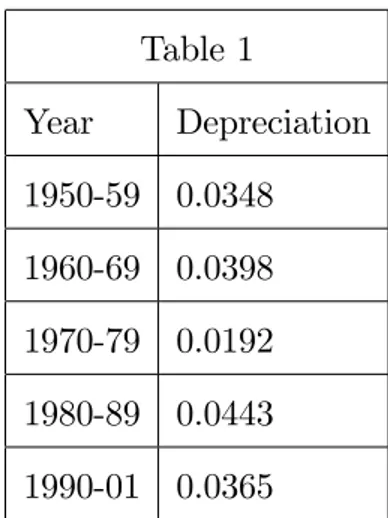
The results are shown in Table 1. We obtain an average depreciation rate of 3.5%
per year. Note that in the 1970s the depreciation rate is slightly reduced, which is then
Table 1
Year Depreciation
1950-59 0.0348
1960-69 0.0398
1970-79 0.0192
1980-89 0.0443
1990-01 0.0365
A possible explanation for the behavior of the depreciation rate during the 1970s and
1980s is that in the 1970s there was a price shock in basic inputs, causing a permanent
change in the relative prices. This situation made the current technologies to be no longer
be optimal in the long run. Consequently, various investment projects were postponed.
2.7.2 Technological Progress, Population Growth, and Distributional
Para-meters
We adjust a determinist and continuous trend to the output per worker series for the
U.S. economy. We obtain g =exp(0:0177) 1, implyingg = 0:1785.
We employ the population growth rate for each country between 1950 and 2000 as
a proxy for the population growth rate n, used in the calculation of the initial capital
according to the methodology developed in subsection 2.4, expression (5). The production
function is CD, then the capital share of income is constant and given by K;C. We use
K;C = 0:4.
2.8
TFP Calculation
Finally, we calculate the productivity for each country based on the following equation:
Ajt =
yjt
k K;C
for the Cobb-Douglas production function, where Ajt is the total factor productivity,
yjt is the output per worker of economy j at time t, kjt is the capital-labor ratio, Hjt
represents the impact of schooling on labor productivity and t= (1 +g)trepresents the
impact of the technological frontier evolution on labor productivity. The construction of
the variables and parameters was described in previous sections .
We then calculate the 81 TFP series, and after estimating all the series, we normalize
the United States productivity in 1950 as 100. We present some graphics below to
illustrate these estimations. The complete series of graphs, with the countries divided by
regions, are presented in the Appendix.4
3
Econometric Model
We use a dynamic log-linear model to model the TFP time-series for all the countries
for which the series are already calculated, and from this model we estimate and test
the dates and the number of structural changes present in each series. Lag variables are
present in econometrics for several reasons, and when e¤ects of variables persist over time
an appropriate model shall include lagged variables. Institution (or TFP) is a variable
which is strongly related to its value in previous periods, hence it is important to allow
for lags when modeling it. Inclusion of lag variables in the model might be explained
for several reasons, for instance, technical and technological reasons may cause delay in
implementing changes in capital-labor compositions, institutions are highly correlated
with values of preceding periods since implementation of public policies could be very
slow, labor contracts are …xed for long periods, etc. Hence, the total factor productivity
is modeled as:
lnAjt =Cj+ jlnAjt 1 +"jt (9)
4When investigating closely the graphs of the series by regions, one can notice evidence of club
where, Ajt is the TFP for the j-th economy at period t, Cj is a constant, and "jt is the
error term, which is assumed to be independent and identically distributed with zero
mean and variance 2
j.
We assume that there is no change in the autoregression coe¢cient. Therefore, for
instance, in a model with a break in the constant, we have the following model:
lnAjt = Cj1+ jlnAjt 1+"jt, if t < Tj (10)
lnAjt = Cj2+ jlnAjt 1+"jt, if t Tj;
where Tj is the break date for a level change in the j-economy.
For a changes in level and trend, the total factor productivity is modeled as:
lnAjt =Cj+gjt+ jlnAjt 1 +"jt: (11)
Thus, if there is a break in the constant and in the time trend:
lnAjt = Cj1+gj1t+ jlnAjt 1+"jt, if < Tj (12)
lnAjt = Cj2+gj2t+ jlnAjt 1+"jt, if Tj;
where gj is the linear time trend coe¢cient and the other parameters have the same
meaning as in equation (9).
3.1
Estimation and Inference
The methods used for estimation and testing for the structural breaks in the TFP series
were proposed by Bai and Perron (1998, 2003). In this section we describe them brie‡y.
Consider the following regression with m breaks and (m+ 1 regimes):
yt =x0t +z
0
forj = 1,...m+ 1. In this model,ytis the dependent variable observed in time t;xt(p 1)
and zt(q 1)are the independent variables, and j (j = 1; :::; m+ 1)are the vectors of
coe¢cients;utis the error term in timet. The indices(T1; :::; Tm), or the points of breaks,
are treated as unknown, as a convention we set T0 = 0 and Tm+1 = T. The purpose is
to estimate the unknown regression coe¢cients together with the break points when T
observations on (yt; xt; zt) are available. This is a partial structural change model, since
is not subject to shifts and is e¤ectively estimated using the entire sample.
The multiple linear regression model (13) can be expressed in the following form:
Y =X +Z +U; (14)
where, Y = (y1; :::; yT)0, X = (x1; :::; xT)0, U = (u1; :::; uT)0, = ( 01; 02; :::; 0m+1), and Z
is the matrix with diagonally partitions Z at the m-partition (T1:::; Tm), that is, Z =
diag(Z1:::; Zm+1) with Zi = (zTi 1+1; :::; zTi)
0. In general, the number of breaksm can be
treated as an unknown variable with true value m0.
The intuition for the estimation is the following: suppose we know the number of
structural breaks ex ante, or we have an upper bound for it. In the case of one change,
for example, we estimate the parameters and by linear regression for all periods in
the sample, with the exception of the …rst and the last ones. Then, we compute the sum
of squared residuals. Finally, the estimated break point is the one which minimizes the
computed sum of squared residuals. In the case with two breaks we estimate the linear
regression for and all combinations (or partitions) with two breaks and compute the
sum of squared residuals for each estimate. Again, the estimated break points are the
ones which minimize the computed sum of squared residuals. The procedure is the same
for larger numbers of breaks.
Formally, for each m-partition(T1; :::; Tm), denotedfTjg, the associated least squares
estimates of and j are obtained by minimizing the sum of squared residuals:
(Y X +Z )0
(Y X +Z ) =
m+1 X
i=1
Ti X
t=T1 1+1
[yt x0t z
0
t i]
2
Let ^ (fTjg) and ^(fTjg) denote the resulting estimates based on the m-partitions
(T1; :::; Tm). Substituting them in the objective function and denoting the resulting sum
of the squared residuals asST(T1; :::; Tm), the estimated break points (T^1; :::;T^m) are such
that
( ^T1; :::;T^m) =argminT1;:::;TmST(T1; :::; Tm); (16)
where the minimization is taken over all partitions (T1; :::; Tm) such that Ti Ti 1 q:
Finally, the regression parameters estimates are the associated least squares estimates at
the estimatedm-partition nT^j
o
;that is, ^ = ^ (nT^j
o
), and^ = ^(nT^j
o
):
Bai and Perron (1998) propose a test for the null hypothesis of l breaks against the
alternative that an additional break exists. Test statistic for testing H0 : m = l versus
H1 : m= l+ 1 is constructed using the di¤erence between the sum of squared residuals
(SSR) associated withlbreaks and those associated withl+ 1breaks.5 The test amounts
to the application of (l + 1) tests of the null hypothesis of no structural breaks versus
the alternative hypothesis of a single change. We conclude for the rejection in favor of a
model with (l+ 1) breaks if the overall minimum value of the sum of squared residuals
(over all segments where an additional break is included) is su¢ciently smaller than the
sum of squared residuals from thel break model. The break date thus selected is the one
associated with this overall minimum. More precisely, the test is de…ned by the equation:
FT(l+ 1 jl) = ST T^1; :::;T^l min
1 i l+1 2infi:
ST T^1; :::;T^i 1; ;T^i; :::;T^l =^2; (17)
where i; =
n
; ^Ti 1+ ( ^Ti T^i 1) T^i ( ^Ti T^i 1) o
and ^2 is a consistent
es-timator of 2 under the null hypothesis.
Intuitively, one can reject the model with l breaks in favor of a model with (l + 1)
breaks if the minimum SSR (over all segments including an additional break) is su¢ciently
lower than the SSR of the model withlbreaks. Intuitively,ST( ^T1; :::;T^l)is the SSR under
5One drawback in the testing procedure is that the test does not formally allow for time trend
the null hypothesis, that is, the SSR of the model adjusted withlbreaks and the in…mum
of ST T^1; :::;T^i 1; ;T^i; :::;T^l is the lowest SSR considering the model with a additional
break, if this additional break is capable of reducing the SSR enough then the test statistic
supLRT(l+ 1 jl) increases and one can reject the null hypothesis of l structural breaks.
We use the methods of estimation and test described in this section for estimating and
testing the number of structural breaks in the TFP for 81 countries.
4
Results
The results for all estimations, which is, all the dates and numbers of structural breaks,
are described in Table 3 in the Appendix, as well as possible explanations for the various
dates. We allow for a maximum of three breaks, and we use a testing signi…cance level
of 5% for all estimations.
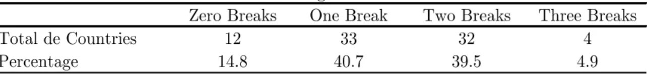
There were 109 detectedstructural breaks, with 12 countries showing zero breaks. The
Table 2 summarizes the results.
Table 2: selected countries
Zero Breaks One Break Two Breaks Three Breaks
Total de Countries 12 33 32 4
Percentage 14.8 40.7 39.5 4.9
Number and Percentage of Structural Breaks
Table 2 shows that about 15% of the countries have zero structural breaks and about
41% of the countries have two breaks6. In addition, about 85% of the countries in the
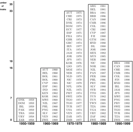
sample present at least one structural change. Figure 1 shows histogram with the number
of breaks per decade. There are 35 breaks in the 80’s and 33 during the 70’s. Most of
the countries that had structural changes in the 80’s are developing countries, and in the
1970-1979 there are a reasonable number of developed countries.
Figure 1: histogram of number of breaks per decade
Number
of ARG 1981
Breaks BEL 1981
AUT 1975 BRA 1981 CHE 1975 BRB 1986 CRI 1973 CAN 1980 DNK 1974 CMR 1986 DOM 1975 COL 1981 ECU 1977 CRI 1980 ESP 1975 CYP 1987 FRA 1974 FJI 1980 GBR 1974 GTM 1981 GRC 1974 HND 1980 IRN 1977 ISL 1988 ITA 1974 JOR 1989 JAM 1973 MEX 1982 JOR 1970 MUS 1985 JPN 1971 NER 1980
KOR 1976 NIC 1988 BRA 1990 LSO 1975 NOR 1981 CAN 1990 AUT 1960 MOZ 1974 NZL 1988 CHE 1991 BEL 1960 NER 1974 PAN 1987 CMR 1994 BOL 1961 NLD 1975 PER 1988 COL 1991 BOL 1968 NIC 1970 PHL 1986 FIN 1990 CYP 1965 NIC 1979 PRY 1981 HND 1993 ESP 1961 NPL 1976 SLV 1980 IRL 1994 IND 1965 NZL 1975 SYR 1984 JAM 1993 KEN 1962 PRT 1974 TTO 1985 JPN 1992 KOR 1963 SWE 1970 TUN 1982 MWI 1995 DNK 1959 MWI 1968 TGO 1971 TUN 1988 PNG 1995 DOM 1959 NZL 1967 TGO 1977 TWN 1985 PRY 1992 IRL 1959 PHL 1960 TUR 1977 TZA 1988 SWE 1990 PAK 1959 PNG 1966 USA 1974 UGA 1984 TGO 1993 THA 1959 SLV 1967 VEN 1971 URY 1982 TUR 1994 URY 1958 VEN 1962 ZAR 1975 ZAF 1982 TZA 1995
0 ZAR 1958 ZWE 1969 ZMB 1977 ZWE 1986 ZWE 1992
1980-1989 1990-1999
7
1950-1959 1960-1969 1970-1979
35 33
18 16
In order to interpret the results we have classi…ed the structural changes into two
groups. The …rst group contains the structural changes caused by internal factors. These
can be institutional changes, internal political changes such as changes in the constitution,
political independence, nationalization of important economic activities,
redemocratiza-tion, or internal economic changes caused, for instance, by joining a trade block.
In the second group are the structural changes caused by external shocks. These can
be described as external economic changes, such as the oil shock in the 1970s and the
shock in the international interest rates in the 1980s. About 53% of the structural breaks
can be explained by institutional changes. Another 29% of the changes can be explained
by external shocks, that is, the oil shock and shock in the international interest rates.
The remaining 18% could not be properly explained.7
As expected, external shocks a¤ect various countries in a systematic fashion, whereas,
7In some cases there is more than one explanation for a break. For example, the break in 1975 in Spain
in general, the breaks associated with internal dynamics do not show strong regularities
across countries. We shall see later that most of the estimated breaks related to internal
factors are downwards, with exception of breaks related to trade, implying that internal
shocks may have very important consequences for economical development and growth.
Out of the 69 countries that presented structural changes, 40 had at least one change
that can be attributed to internal factors. Most of these countries, about 70%, are
developing countries. The majority of the breaks were caused by changes in constitutions.
Twenty one countries experienced a change in constitution.
As observed by Jones and Olken (2007), economic changes such as trade are important
causes of accelerations. However, from all the detected breaks related with internal factors
only 8 could possibly be explained by this argument. Therefore, there is evidence that
in-ternal political changes are extremely important for explaining breaks in TFP. Examples
of countries with changes in constitutions include: Brazil, Canada, Cameroon, Honduras,
Nicaragua, New Zealand, El Salvador, and South Africa, among others. Therefore, the
results complement Jones and Olken (2007) by giving strong evidence that the majority
of the structural changes can be attributed to internal factors, more speci…cally to
in-stitutional and political changes such as political independence or the adoption of new
constitution, and therefore, internal shocks are the main factors responsible for structural
changes in the TFP series.
Two regularities about the external shocks structural changes were detected. The …rst
observation is that changes caused by the oil shock a¤ected mainly developed countries
such as the United States and Western Europe countries like Great Britain, Austria,
France, Denmark, etc in the middle of the 1970s. Secondly, various Latin American
countries such as Argentina, Brazil, Costa Rica and Mexico, among others, su¤ered from
the shock in the international interest rates during the 1980s. It is likely that the …nancing
policy put in place in response to the oil shock by several Latin American countries set the
foundation for future vulnerability to the shock in interest rates. Therefore, the results
presented here for TFP are in accordance with the results presented by Ben-David and
the developed countries are related to the …rst oil shock, the meltdown for developing
countries commenced with the second oil shock and the start of the debt crisis.
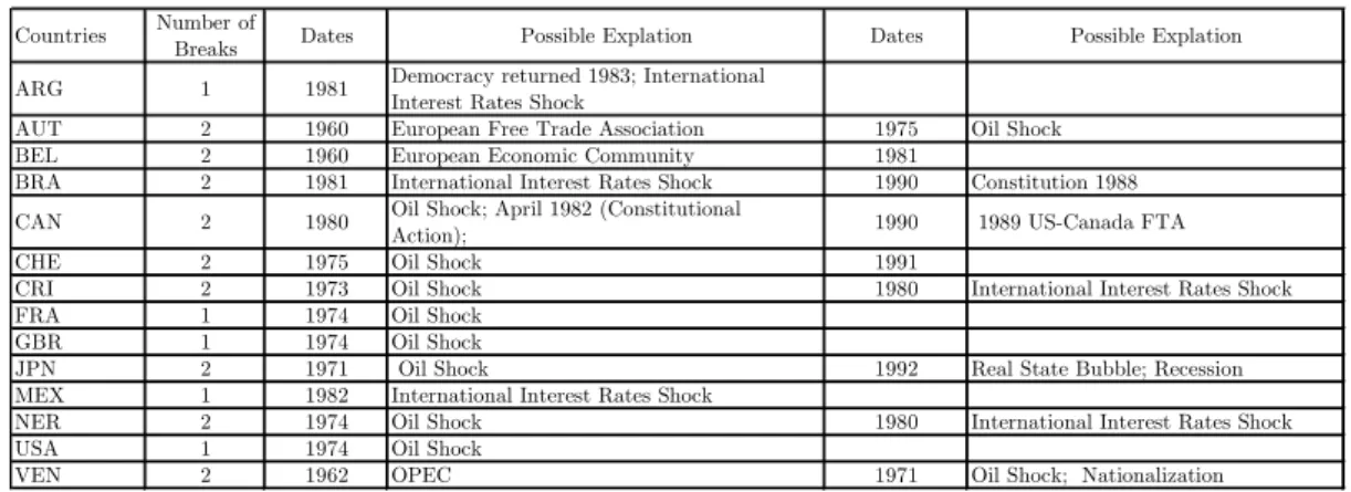
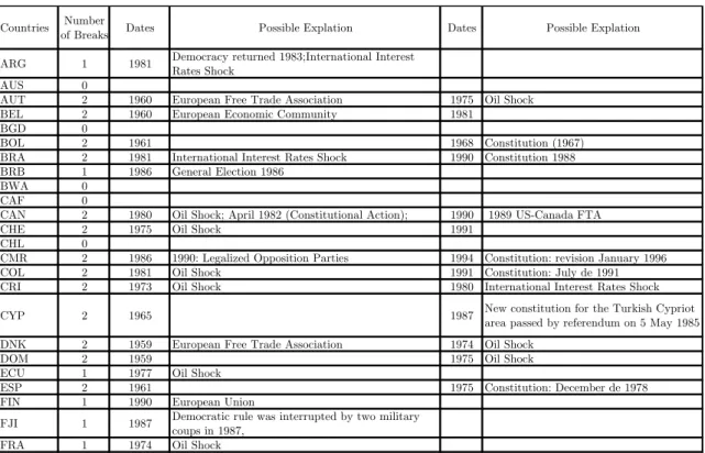
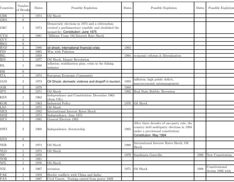
Table 3 below presents, for a selected group of countries, the dates and possible
expla-nation of breaks. As previously explained, there are many countries in which productivity
was hurt because of the e¤ects of the oil shocks. In some developing countries such as
Brasil, Argentina and Costa Rica there are TFP breaks in the early eighties that are,
most likely, caused by Volcker’s interest rate shock and the …nancial crises that followed
it. As a matter of fact, all but one Latin America country in our sample had at least one
productivity break in the eighties or late seventies. And all of them implied productivity
reduction or slowdown afterward.
Table 3: selected countries
Countries Number of
Breaks Dates Possible Explation Dates Possible Explation
ARG 1 1981 Democracy returned 1983; International
Interest Rates Shock
AUT 2 1960 European Free Trade Association 1975 Oil Shock
BEL 2 1960 European Economic Community 1981
BRA 2 1981 International Interest Rates Shock 1990 Constitution 1988
CAN 2 1980 Oil Shock; April 1982 (Constitutional
Action); 1990 1989 US-Canada FTA
CHE 2 1975 Oil Shock 1991
CRI 2 1973 Oil Shock 1980 International Interest Rates Shock
FRA 1 1974 Oil Shock
GBR 1 1974 Oil Shock
JPN 2 1971 Oil Shock 1992 Real State Bubble; Recession
MEX 1 1982 International Interest Rates Shock
NER 2 1974 Oil Shock 1980 International Interest Rates Shock
USA 1 1974 Oil Shock
VEN 2 1962 OPEC 1971 Oil Shock; Nationalization
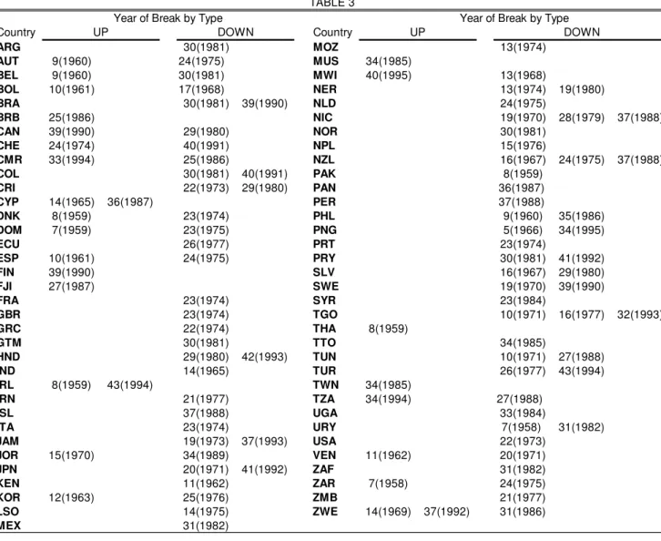
In regards to whether the breaks shift the TFP time series upwards or downwards,
we classify the breaks into two categories, say UP and DOWN. The results are shown in
Table A.2 in the appendix
UP breaks are those in which the regime after the break is larger than the regime
was before.8 DOWN breaks correspond to the opposite case. Table 3 shows that most
of the TFP breaks are DOWN breaks, i.e., about 75% of the breaks (82 out of 109)
are downward types of changes, and only about 25% of the changes (27 out of 109) are
upward. Upward changes, are strongly related with international trade. For example,
8When we consider only a change in the intercept, UP means that the intercept coe¢cient is higher
the estimated structural break in Canada in 1990 could be explained by the US-Canada
Free Trade Agreement; the break in 1960 in Belgium and Austria that can possibly be
explained by the formation of the European Economic Community and the European
Free Trade Association, respectively.
However, the majority of the breaks are downwards. The internal factor changes in
government regimes, such as political independence or adopting a new constitutions are
the main factors responsible for such structural changes in the TFP series. The majority
of these breaks were caused by changes in constitution and among the 21 breaks related
with constitutions only 3 are upwards, say Cameroon, Cyprus, and Malawi. In many
cases, this is so because new constitutions are adopted after revolutions or periods of civil
unrest, and these episodes, in general, impact production and productivity negatively.
From the external factor point of view all the estimated breaks are downwards, with
the exception of Switzerland showing an upward break in 1975 which could be related to
the oil shock. Therefore, overall, after the changes caused by the oil shock, the
productiv-ity declines, since most countries are consumers of this product. However, in our sample
there are also countries that are oil producers and for these countries the productivity
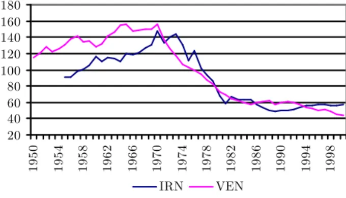
should increase in the case of a positive terms-of-trade shock. Yet, there are two cases
we should analyze individually, Venezuela and Iran. Both countries are oil producers
and exhibit structural breaks related to the oil shock in the 1970s, nevertheless their
productivities decline sharply after this shock.
Figure 2: TFP Venezuela and Iran
20 40 60 80 100 120 140 160 180
1950 1954 1958 1962 1966 1970 1974 1978 1982 1986 1990 1994 1998
A possible interpretation for the phenomena occurring after adopting a new
consti-tution or that resulted in productivity decline for Iran and Venezuela is given by Rodrik
(1999) by arguing that social con‡icts might explain the great drop in the TFP of these
countries. This result indicates that after a break, the TFP tends to decrease,
imply-ing that institutional rearrangements, external shocks, or internal shocks could be costly
and di¢cult to recover from. Another possible interpretation, in the case of Venezuela,
can be found in Cole, Ohanian, Riascos and Schmitz (2005), that show that after the
nationalization of oil and mining in the seventies, productivity dropped signi…cantly9.
5
Final Considerations
The purpose of this work is to present estimates for structural breaks in total factor
productivity within countries, and to identify, whenever possible, episodes in the
polit-ical and economic history of these countries that may explain the structural breaks in
question. The results suggest that about 85% of the countries in a sample of 81 countries
experienced at least one structural change, totaling 109 observed breaks. Among these,
about 53% are associated with internal shocks, 29% are associated with external shocks
and the other 18% could not be appropriately explained.
The structural changes occur mainly due to internal factors. Changes in government
regimes, political independence or the adoption of a new Constitution are responsible for
structural changes in the TFP series. Out of 69 countries with structural changes, 40
exhibit at least one break related to internal factors, and most of these breaks occurred in
developing countries. In addition, the most common internal factor triggering structural
breaks is a new constitution.
Two factors are common to various countries, the oil shock and the shock in
inter-national interest rates, causing structural breaks in various economies. The oil shock
a¤ected particularly the United States and the Western European countries, while,
prob-ably due to their …nancing policies, the Latin American countries were mostly a¤ected
9As for Iran, the Islamic Revolution of 1979 must had played an important role in the productivity
by the international interest rates shock. On the other hand, the dates of the structural
breaks related to the internal dynamics of each country do not show a common pattern.
In addition, the results indicate that the majority of the breaks are downward, and after
a break the TFP tends to decrease, implying that institutional rearrangements, external
shocks, or internal shocks in general could be costly and di¢cult to recover from.
6
References
Bai, J.and Perron, P. (1998) “Estimating and Testing Linear Models with Multiple
Struc-tural Changes”, Econometrica, 66, 47-78.
Bai, J. and Perron, P. (2003) “Computation and Analysis of Multiple Structural Break
Models,”Journal of Applied Econometrics, 18, 1-22.
Barro, R. and Lee, J. W. (2000) “International Data on Educational Attainment:
Updates and Implications,” NBER Working Paper #7911.
Ben-David, D. and Papell, D. H. (1998) "Slowdowns and Meltdowns: Postwar Growth
Evidence from 74 Countries," The Review of Economics and Statistics, 80, 561-571.
Bils, M. and Klenow, P. (2000) “Does Schooling Cause Growth?”,American Economic
Review,90, 1160-1183.
Ciccone, A. and Peri, G. (2006) “Identifying Human Capital Externalities: Theory
with Applications,” Review of Economic Studies, 73, 381-412.
Cole, H. L., Ohanian, L. E., Riascos, A. and Schmitz, J., (2005). "Latin America in
the rearview mirror,"Journal of Monetary Economics, 52, 69-107.
Gollin, D. (2002) “Getting Income Share Right”, Journal of Political Economy, 110,
458-474.
Hulten, Charles. R. (2001) “Total Factor Productivity: A Short Biography”, in New
Developments in Productivity Analysis, Charles R. Hulten, Edwin R. Dean, and Michael
J. Harper, eds., Studies in Income and Wealth, vol. 63, The University of Chicago Press
for the National Bureau of Economic Research, Chicago, 1-47.
Output per Worker than Others?” Quarterly Journal of Economics, February, 114,
83-116.
Jones, B. and Olken, B. (2007) “The Anatomy of Start-Stop Growth,”The Review of
Economics and Statistics, forthcoming.
Klenow, P. and Rodriguez-Clare, A. (1997) “The Neoclassical Revival in Growth
Economics: Has It Gone Too Far?” NBER Macroeconomics Annual 1997, B. Bernanke
and J. Rotemberg ed., Cambridge, MA: MIT Press, 73-102
Krusell, P. and Rios-Rull, J. V. (1996) “Vested Interests in a Positive Theory of
Stagnation and Growth”, The Review of Economic Studies, April , 63, 301-329.
Lagos, R. (2006) “A Model of TFP,” Review of Economics Studies, 73, 983-1007.
Mankiw, G., Romer, D. and Weil, D. (1992) “A Contribution to the Empirics of
Economic Growth,” Quarterly Journal of Economics, 107, 407-437.
Moretti, E. (2004) “Estimating the social return to higher education: evidence from
longitudinal and repeated cross-sectional data ,” Journal of Econometrics, 121, 175-212.
Parente, S. L. and Prescott, E. (1999) “Monopoly Rights: A Barrier to Riches” The
American Economic Review, 89, 1216-1233.
Pessoa, S. A., Pessoa, S. M. and Rob, R.(2003). “Price Elasticity of Investiment: a
Panel Data Approach”, University of Pennsylvania, (mimeo).
Prescott, E. (1998) “Lawrence R. Klein Lecture 1997 Needed: A Theory of Total
Factor Productivity”, International Economic Review, 39, 525-551.
Psacharopoulos, G. (1994) “Returns to Investiment in Education: A Global Update”,
World Development, 22, 1325-1343.
Rodrik, D. (1999) “Where Did All The Growth Go? External Shocks, Social Con‡ict,
7
Appendix
Table A.1: Legend
1 ARG Argentina 41 KEN Kenya
2 AUS Australia 42 KOR Korea, Republic of
3 AUT Austria 43 LSO Lesotho
4 BEL Belgium 44 MEX Mexico
5 BGD Bangladesh 45 MOZ Mozambique
6 BOL Bolivia 46 MUS Mauritius
7 BRA Brazil 47 MWI Malawi
8 BRB Barbados 48 MYS Malaysia
9 BWA Botswana 49 NER Niger
10 CAF Central African Republic 50 NIC Nicaragua
11 CAN Canada 51 NLD Netherlands
12 CHE Switzerland 52 NOR Norway
13 CHL Chile 53 NPL Nepal
14 CMR Cameroon 54 NZL New Zealand
15 COL Colombia 55 PAK Pakistan
16 CRI Costa Rica 56 PAN Panama
17 CYP Cyprus 57 PER Peru
18 DNK Denmark 58 PHL Philippines
19 DOM Dominican Republic 59 PNG Papua New Guinea
20 ECU Ecuador 60 PRT Portugal
21 ESP Spain 61 PRY Paraguay
22 FIN Finland 62 SEN Senegal
23 FJI Fiji 63 SGP Singapore
24 FRA France 64 SLV El Salvador
25 GBR United Kingdom 65 SWE Sweden
26 GHA Ghana 66 SYR Syria
27 GRC Greece 67 TGO Togo
28 GTM Guatemala 68 THA Thailand
29 GUY Guyana 69 TTO Trinidad &Tobago
30 HKG Hong Kong 70 TUN Tunisia
31 HND Honduras 71 TUR Turkey
32 IND India 72 TWN Taiwan
33 IRL Ireland 73 TZA Tanzania
34 IRN Iran 74 UGA Uganda
35 ISL Iceland 75 URY Uruguay
36 ISR Israel 76 USA USA
37 ITA Italy 77 VEN Venezuela
38 JAM Jamaica 78 ZAF South Africa
39 JOR Jordan 79 ZAR Congo, Dem. Rep.
40 JPN Japan 80 ZMB Zambia
7.1
K
0Starting from the capital law of motion:
K0 = (1 )K 1+I 1;
and
K 1 = (1 )K 2+I 2;
substituting
K0 = (1 ) [(1 )K 2+I 2] +I 1
= (1 )2K
2+ (1 )I 2+I 1
= (1 )2[(1 )K 3+I 3] + (1 )I 2+I 1
= (1 )3K 3+ (1 )2I 3+ (1 )I 2+I 1
= :::
= (1 )TK T + T
X
j=1
(1 )j 1I j
and assuming,
I j =I0(1 +g) j(1 +n) j;
then
K0 = (1 )TK T +
I0
(1 +g)(1 +n)
T 1
X
j=0
1
(1 +g)(1 +n)
j
K0 =
I0
(1 +g)(1 +n)
1
1 1
(1+g)(1+n)
K0 =
I0
g+n+ng+
7.2
Graphs
South America 1
0 20 40 60 80 100 120
1950 1952 1954 1956 1958 1960 1962 1964 1966 1968 1970 1972 1974 1976 1978 1980 1982 1984 1986 1988 1990 1992 1994 1996 1998 2000
ARG BRA CHL ECU PER PRY URY
South America 2
0 20 40 60 80 100 120 140 160 180
1950 1952 1954 1956 1958 1960 1962 1964 1966 1968 1970 1972 1974 1976 1978 1980 1982 1984 1986 1988 1990 1992 1994 1996 1998 2000
BOL COL GUY VEN North America 0 20 40 60 80 100 120
19501952195419561958196019621964196619681970197219741976197819801982198419861988199019921994199619982000 CAN MEX USA Central America 0 20 40 60 80 100 120 140 160
1950 1952 1954 1956 1958 1960 1962 1964 1966 1968 1970 1972 1974 1976 1978 1980 1982 1984 1986 1988 1990 1992 1994 1996 1998 2000
Caribbean 0 20 40 60 80 100 120 140
1950 1952 1954 1956 1958 1960 1962 1964 1966 1968 1970 1972 1974 1976 1978 1980 1982 1984 1986 1988 1990 1992 1994 1996 1998 2000
TTO BRB DOM JAM
Western Europe 1
0 20 40 60 80 100 120
1950 1952 1954 1956 1958 1960 1962 1964 1966 1968 1970 1972 1974 1976 1978 1980 1982 1984 1986 1988 1990 1992 1994 1996 1998 2000
AUT BEL CHE GBR IRL NLD
Western Europe 2
0 20 40 60 80 100 120
19501952195419561958196019621964196619681970197219741976197819801982198419861988199019921994199619982000
ESP FRA ITA PRT
Western Europe 3
0 10 20 30 40 50 60 70 80 90 100
1950 1952 1954 1956 1958 1960 1962 1964 1966 1968 1970 1972 1974 1976 1978 1980 1982 1984 1986 1988 1990 1992 1994 1996 1998 2000
DNK FIN ISL NOR SWE AFRICA 1 0 50 100 150 200 250
19501952195419561958196019621964196619681970197219741976197819801982198419861988199019921994199619982000
BWA CAF GHA MOZ NER NPL UGA KEN LSO AFRICA 2 0 20 40 60 80 100 120 140 160
1950 1952 1954 1956 1958 1960 1962 1964 1966 1968 1970 1972 1974 1976 1978 1980 1982 1984 1986 1988 1990 1992 1994 1996 1998 2000
Eastern
0 20 40 60 80
100 120 140 160 19 50 19 52 19 54 19 56 19 58 19 60 19 62 19 64 19 66 19 68 19 70 19 72 19 74 19 76 19 78 19 80 19 82 19 84 19 86 19 88 19 90 19 92 19 94 19 96 19 98 20 00 BGD IRN ISR PAK T UN IND JOR S YR A sian
0 20 40 60 80
100 120 140
19 50 19 52 19 54 19 56 19 58 19 60 19 62 19 64 19 66 19 68 19 70 19 72 19 74 19 76 19 78 19 80 19 82 19 84 19 86 19 88 19 90 19 92 19 94 19 96 19 98 Mediterranean
0 20 40 60 80
100 120 1950 1952 1954 1956 1958 1960 1962 1964 1966 1968 1970 1972 1974 1976 1978 1980 1982 1984 1986 1988 1990 1992 1994 1996 1998 2000 CYP GRC TUR Oceania
0 20 40 60 80 100 120
Table A.2: Year and Type of Break
Country Country
ARG 30(1981) MOZ 13(1974)
AUT 9(1960) 24(1975) MUS 34(1985)
BEL 9(1960) 30(1981) MWI 40(1995) 13(1968)
BOL 10(1961) 17(1968) NER 13(1974) 19(1980)
BRA 30(1981) 39(1990) NLD 24(1975)
BRB 25(1986) NIC 19(1970) 28(1979) 37(1988)
CAN 39(1990) 29(1980) NOR 30(1981)
CHE 24(1974) 40(1991) NPL 15(1976)
CMR 33(1994) 25(1986) NZL 16(1967) 24(1975) 37(1988)
COL 30(1981) 40(1991) PAK 8(1959)
CRI 22(1973) 29(1980) PAN 36(1987)
CYP 14(1965) 36(1987) PER 37(1988)
DNK 8(1959) 23(1974) PHL 9(1960) 35(1986)
DOM 7(1959) 23(1975) PNG 5(1966) 34(1995)
ECU 26(1977) PRT 23(1974)
ESP 10(1961) 24(1975) PRY 30(1981) 41(1992)
FIN 39(1990) SLV 16(1967) 29(1980)
FJI 27(1987) SWE 19(1970) 39(1990)
FRA 23(1974) SYR 23(1984)
GBR 23(1974) TGO 10(1971) 16(1977) 32(1993)
GRC 22(1974) THA 8(1959)
GTM 30(1981) TTO 34(1985)
HND 29(1980) 42(1993) TUN 10(1971) 27(1988)
IND 14(1965) TUR 26(1977) 43(1994)
IRL 8(1959) 43(1994) TWN 34(1985)
IRN 21(1977) TZA 34(1994) 27(1988)
ISL 37(1988) UGA 33(1984)
ITA 23(1974) URY 7(1958) 31(1982)
JAM 19(1973) 37(1993) USA 22(1973)
JOR 15(1970) 34(1989) VEN 11(1962) 20(1971)
JPN 20(1971) 41(1992) ZAF 31(1982)
KEN 11(1962) ZAR 7(1958) 24(1975)
KOR 12(1963) 25(1976) ZMB 21(1977)
LSO 14(1975) ZWE 14(1969) 37(1992) 31(1986)
MEX 31(1982)
TABLE 3
Year of Break by Type Year of Break by Type
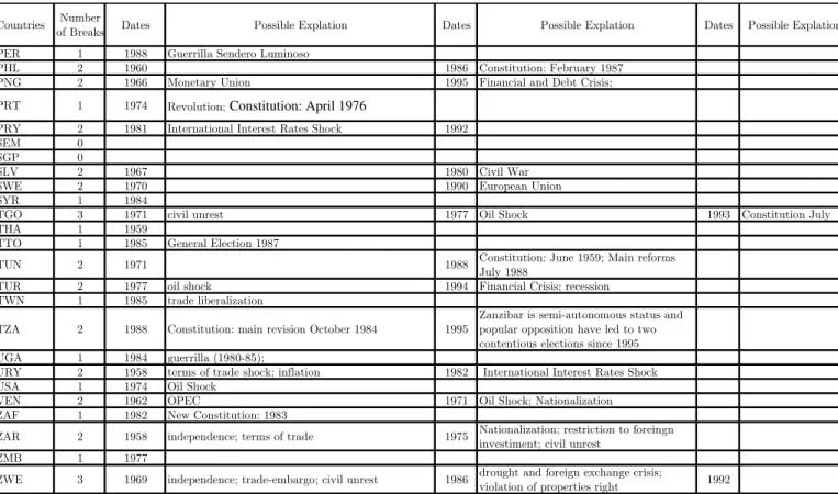
Table A.3: Possible Causes of Breaks
Countries Number
of Breaks Dates Possible Explation Dates Possible Explation
ARG 1 1981 Democracy returned 1983;International Interest Rates Shock
AUS 0
AUT 2 1960 European Free Trade Association 1975 Oil Shock
BEL 2 1960 European Economic Community 1981
BGD 0
BOL 2 1961 1968 Constitution (1967)
BRA 2 1981 International Interest Rates Shock 1990 Constitution 1988
BRB 1 1986 General Election 1986
BWA 0
CAF 0
CAN 2 1980 Oil Shock; April 1982 (Constitutional Action); 1990 1989 US-Canada FTA
CHE 2 1975 Oil Shock 1991
CHL 0
CMR 2 1986 1990: Legalized Opposition Parties 1994 Constitution: revision January 1996
COL 2 1981 Oil Shock 1991 Constitution: July de 1991
CRI 2 1973 Oil Shock 1980 International Interest Rates Shock
CYP 2 1965 1987 New constitution for the Turkish Cypriot
area passed by referendum on 5 May 1985
DNK 2 1959 European Free Trade Association 1974 Oil Shock
DOM 2 1959 1975 Oil Shock
ECU 1 1977 Oil Shock
ESP 2 1961 1975 Constitution: December de 1978
FIN 1 1990 European Union
FJI 1 1987 Democratic rule was interrupted by two military coups in 1987,
Table A.3: Possible Causes of Breaks (cont.)
Countries Number
of Breaks Dates Possible Explation Dates Possible Explation Dates Possible Explation
GBR 1 1974 Oil Shock
GHA 0
GRC 1 1974
Democratic elections in 1974 and a referendum created a parliamentary republic and abolished the monarchy;Constitution: June 1975
GTM 1 1981 Military Coup; Oil/Interest Rate Shock
GUY 0
HKG 0
HND 2 1980 oil shock; international financial crisis 1993 IND 1 1965 War with Pakistan
IRL 2 1959 1994 economic reforms & liberalization
IRN 1 1977 Oil Shock, Islamic Revolution
ISL 1 1988 inflation; stabilization plan; crisis in the fishing industry
ISR 0
ITA 1 1974 European Economic Community
JAM 2 1973 Oil Shock; domestic violence and dropoff in tourism. 1993 inflation; high public deficit, macroeconomic mismanagement
JOR 2 1970 1989
JPN 2 1971 Oil Shock 1992 Real State Bubble; Recession
KEN 1 1962 Independence and Constitution: December 1963 (from UK);
KOR 2 1963 Industrial Policy 1976 Oil Shock
LSO 1 1975 Oil Shock
MEX 1 1982 International Interest Rates Shock MOZ 1 1974 Independence: June 1975 MUS 1 1985 General Election 1983
MWI 2 1968 Independence; dictatorship 1995
After three decades of one-party rule, the country held multiparty elections in 1994 under a provisional constitution;
Constitution: May 1994
MYS 0
NER 2 1974 Oil Shock 1980 International Interest Rates Shock; Oil Shock
NLD 1 1975 Oil Shock
NIC 3 1970 1979 Sandinista Guerrilla 1988 New Constitution;
NOR 1 1981
NPL 1 1976 Oil Shock
NZL 3 1967 recession 1975 Oil Shock 1988 Constitutional
Action 1986 with PAK 1 1959 Border conflicts with China and India;
Table A.3: Possible Causes of Breaks (cont.)
Countries Number
of Breaks Dates Possible Explation Dates Possible Explation Dates Possible Explation
PER 1 1988 Guerrilla Sendero Luminoso
PHL 2 1960 1986 Constitution: February 1987
PNG 2 1966 Monetary Union 1995 Financial and Debt Crisis;
PRT 1 1974 Revolution;Constitution: April 1976
PRY 2 1981 International Interest Rates Shock 1992
SEM 0
SGP 0
SLV 2 1967 1980 Civil War
SWE 2 1970 1990 European Union
SYR 1 1984
TGO 3 1971 civil unrest 1977 Oil Shock 1993 Constitution July
THA 1 1959
TTO 1 1985 General Election 1987
TUN 2 1971 1988 Constitution: June 1959; Main reforms
July 1988
TUR 2 1977 oil shock 1994 Financial Crisis; recession
TWN 1 1985 trade liberalization
TZA 2 1988 Constitution: main revision October 1984 1995
Zanzibar'is semi-autonomous status and popular opposition have led to two contentious elections since 1995
UGA 1 1984 guerrilla (1980-85);
URY 2 1958 terms of trade shock; inflation 1982 International Interest Rates Shock
USA 1 1974 Oil Shock
VEN 2 1962 OPEC 1971 Oil Shock; Nationalization
ZAF 1 1982 New Constitution: 1983
ZAR 2 1958 independence; terms of trade 1975 Nationalization; restriction to foreingn investiment; civil unrest
ZMB 1 1977
ZWE 3 1969 independence; trade-embargo; civil unrest 1986 drought and foreign exchange crisis;