Análise de novos modelos matemáticos para o problema de planejamento da expansão de sistemas de transmissão

MOHSEN RAHMANI

ANÁLISE DE NOVOS MODELOS MATEMÁTICOS PARA O

PROBLEMA DE PLANEJAMENTO DA EXPANSÃO DE SISTEMAS DE

TRANSMISSÃO

Ilha Solteira 2013

UNIVERSIDADE ESTADUAL PAULISTA “Júlio de Mesquita Filho”

UNESP

–

CAMPUS de ILHA SOLTEIRA

MOHSEN RAHMANI

ANÁLISE DE NOVOS MODELOS MATEMÁTICOS PARA O

PROBLEMA DE PLANEJAMENTO DA EXPANSÃO DE SISTEMAS DE

TRANSMISSÃO

Rubén Augusto Romero Lázaro Orientador

Marcos Julio Rider Flores Coorientador

Ilha Solteira 2013

Tese apresentada ao Programa de Pós-Graduação em Engenharia Elétrica da

Universidade Estadual Paulista “Júlio de

Mesquita Filho” – UNESP, Campus de Ilha

FICHA CATALOGRÁFICA

Elaborada pela Seção Técnica de Aquisição e Tratamento da Informação Serviço Técnico de Biblioteca e Documentação da UNESP - Ilha Solteira.

Rahmani, Mohsen.

R147a Análise de novos modelos matemáticos para o problema de planejamento da expansão de sistemas de transmissão / Mohsen Rahmani. – Ilha Solteira: [s.n.], 2013 142 f. : il.

Tese (doutorado) - Universidade Estadual Paulista. Faculdade de Engenharia de Ilha Solteira. Área de conhecimento: Automação, 2013

Orientador: Rubén Augusto Romero Lázaro Coorientador: Marcos Julio Rider Flores Inclui bibliografia

1. Planejamento multiestágio de sistemas de transmissão. 2. Modelo disjuntivo reduzido. 3. Sistema de numeração binária.4. GRASP (Sistema operacional de computador). 5. Compensação série fixa.

DEDICO

A minha querida e amada esposa Leili e a minha filha Sophia pelo amor, compreensão e incentivo que permitiram o desenvolvimento deste trabalho.

Acknowledgment

I would like to thank Professor Rubén Romero for his continuous advice and mentorship. His comments and advice have been invaluable and will serve me for a lifetime. This thesis was prepared with a sense of ambition and innovation that would have been impossible to attain without his leadership.

I also thank professor Marcos Julio Rider Flores for his patience, support and wise counsel. My sincere thanks also to Professors José Roberto Sanches Mantovani, Antônio Padilha Feltrin, Sergio Azevedo de Oliveira and Edgar Manuel Carreño.

I also thank the rest of my thesis committee: professor Sergio Luis Haffner, professor Gerson Couto de Oliveira, professor Antônio César Baleeiro Alves.

I am grateful to the State University of São Paulo, which provided me with a fantastic working environment to pursue my goals.

I also thank the University of Florida, Center of Applied Optimization (CAO), for providing an excellent working environment. My special thanks go to Prof. Panos Pardalos, who working environment which permitted me to pursue my goals.

I thank all the members of LaPSSE for their support and for helping me learning Portuguese. Special thanks to my friends Emivan da Silva, Dercio Braga Santos, Fernanda Pereira Silva, Carlos Dornellas.

I also thank Mahdi Pourakbari and Hamid Khorasani for helping and accompanying me during my doctoral studies. I value their friendship and support as well.

Generous funding was provided by the FEPISA and FAPESP. Without their economic support, this thesis would never have been completed.

And finally, special thanks to my wife Leili whose dedication, love and persistent confidence in me has provided me with indispensable support. I owe a debt to her for her confidence in joining me to do my doctorate. I would also thank to our families for their continuous encouragement and support during all stages of my life.

MOHSEN RAHMANI

STUDY OF NEW MATHEMATICAL MODELS FOR TRANSMISSION

EXPANSION PLANNING PROBLEM

Ilha Solteira 2013

UNIVERSIDADE ESTADUAL PAULISTA “Júlio de Mesquita Filho”

UNESP

–

CAMPUS de ILHA SOLTEIRA

MOHSEN RAHMANI

STUDY OF NEW MATHEMATICAL MODELS FOR TRANSMISSION

EXPANSION PLANNING PROBLEM

A dissertation submitted in partial fulfillment of the requirements for the degree of Doctor of Philosophy in Electrical Engineering in the Electrical Engineering Faculty of Ilha Solteira UNESP, São Paulo, Brazil.

Committee in charge:

Professor Rubén Augusto Romero Lázaro Professor Sergio Luis Haffner

Professor Gerson Couto de Oliveira Professor Antônio César Baleeiro Alves Professor José Roberto Sanches Mantovani

RESUMO

O estado da arte em modelagem matemática do problema de planejamento da expansão de sistemas de transmissão (TEP) é analisado nesta tese de doutorado. É proposto um novo modelo linear disjuntivo para o problema TEP baseado no conceito de sistemas de numeração binária para transformar o modelo linear disjuntivo convencional em um problema com um número de variáveis binárias e contínuas muito menores, assim como do número de restrições relacionadas com essas variáveis. Também é usada a fase construtiva da metaheurística GRASP e restrições adicionais, encontradas da generalização do equilibrio de fluxo de potência em uma barra ou conjunto de barras para reduzir o espaço de busca. Os resultados mostram a importância da estratégia de redução do espaço de busca do problema TEP para resolver os modelos de transporte e linear disjuntivo. O problema TEP multiestágio é modelado como um problema de programação linear binária mista e resolvido usando um solver do tipo branch and bound comercial com tempos de processamento relativamente baixos. Outro tópico pesquisado foi a alocação de dispositivos FACTS tais como os capacitores fixos em série (FSCs) para aproveitar melhor a capacidade de transmissão das linhas e adiar ou reduzir o investimento em novas linhas de transmissão em um ambiente de planejamento multiestágio. Assim, pode ser esperado uma excelente relação custo/benefício da integração de dispositivos FSCs no planejamento multiestágio da expansão de sistemas de transmissão. Os resultados encontrados usando alguns sistemas testes mostram que a inclusão de FSCs no problema TEP é uma estratégia válida e efetiva em investimento para as empresas transmissoras e para os responsáveis da expansão nacional do sistema elétrico.

ABSTRACT

State-of-the-art models for transmission expansion planning problem are provided in this thesis. A new disjunctive model for the TEP problem based on the concept of binary numerical systems is proposed in order to transform the conventional disjunctive model to a problem with many fewer binary and continuous variables as well as connected constraints. The construction phase of a greedy randomized adaptive search procedure (GRASP-CP) together with fence constraints, obtained from power flow equilibrium, are employed in order to reduce search space. The studies demonstrate that the proposed search space reduction strategy, has an excellent performance in reducing the search space of the transportation model and reduced disjunctive model of TEP problem. The multistage TEP problem is modeled as a mixed binary linear programming problem and solved using a commercial branch and bound solver with relatively low computational time. Another topic studied in this thesis, is the allocation of FACTS devices in TEP problem. FACTS devices such as fixed series capacitors (FSCs) are considered in the multistage TEP problem to beter utilize the whole transfer capacity of the network and, consequently, to postpone or reduce the investment in new transmission lines. An excellent benefit-cost ratio can be expected from integration of FSC in multistage transmission expansion planning. The results obtained by using some real test systems indicate that the inclusion of FSCs in the TEP problem is a viable and cost-effective strategy for transmission utilities and national planning bureaus.

LIST OF FIGURES

Figure 1 - The model and equations for power balance in the DC model with power losses 29 Figure 2 - Transmission lines model between two buses in the disjunctive model of TEP

problem 32 Figure 3 - Comparison between candidate lines in the disjunctive model and the reduced

disjunctive model 43

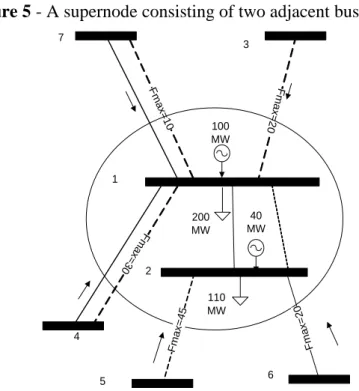
Figure 4 - A generic system bus with neighboring buses and lines 46 Figure 5 - A supernode consisting of two adjacent buses 50 Figure 6 - Pseudo code of GRASP-CP for the static TEP problem using the hybrid

model 55 Figure 7 - Pseudo code of domain reduction of the TEP problem using GRASP-CP 57 Figure 8 - The Garver system with the base case topology and optimum solution 59 Figure 9 - GRASP-CP for reducing the domain of integer variables in the Garver system

(DC model) 59

Figure 10 - Simplified structure of a fixed series capacitor 64 Figure 11 - General model for a transmission corridor with existing lines, candidate lines

and FSCs in a static model of TEP with FSC 65

Figure 12 - General model for a transmission corridor with existing lines, candidate lines

and FSCs 67

Figure 13 - Installed lines for the IEEE-24 bus system in TEP without FSC and with N-1

contingencies in lines 95

Figure 14 - Installed lines and FSCs for the IEEE-24 bus system in TEP with FSC and with

N-1 contingency in lines and FSCs 96

Figure 15 - Installed lines and FSCs for Colombian 93-bus bus system in TEP with FSC 100

Figure 16 - The π model for a transmission line 113

Figure 17 - The model and equations for active and reactive power in a system node 115

Figure 18 - Garver system base line 119

Figure 19 - The Southern Brazilian system 121

Figure 20 - Colombian 93 bus system initial topology 126

L

T

Table 1 - Candidate lines modeling in the reduced disjunctive model 42 Table 2 - The set of constraints obtained using Figure 5 and equation (17b) 50 Table 3 - GRASP-CP procedure for reducing the search space of the DC model of the TEP

problem in the Garver system 58

Table 4 - Southern Brazilian system with generation rescheduling 80 Table 5 - Southern Brazilian system without generation rescheduling 81 Table 6 - North-Northeast Brazilian system without generation rescheduling and with base

case topology for Plan 2002 83

Table 7 - North-Northeast Brazilian system without generation rescheduling and without

base case topology for Plan 2002. 84

Table 8 - North-Northeast Brazilian system without generation rescheduling, with base case

topology for Plan 2008 85

Table 9 - North-Northeast Brazilian system without generation rescheduling, without base

case topology for Plan 2008 86

Table 10 - Results of static TEP for Garver, South-Brazilian and Colombian networks 89 Table 11 - Results of static TEP for Brazilian North-Northeast 89 Table 12 - Results of MTEP for the Colombian system 91 Table 13 - Results of MTEP for the Brazilian North-Northeast 92 Table 14 - Contingency list in the IEEE-24 bus system 94 Table 15 - Power Flow between Region 1 and 2 of the IEEE 24-Bus System 97 Table 16 - Power flow in transmission lines for the Colombian system 99

Table 17 - Garver system bus data for TEP 120

Table 18 - Garver system transmission lines data 120

Table 19 - Southern Brazilian bus system data 122

L

A

AC Alternating current

AMPL A mathematical programming language BNS Binary numeral system

DC Direct current

DM Disjunctive model representation of the DC TEP problem GRASP Greedy randomized adaptive search procedure

GRASP-CP Greedy randomized adaptive search procedure construction phase HLM Hybrid linear model

KCL Kirchhoff current law

LP Linear Programming

MILP Mixed integer linear programming Problem MTEP Multistage transmission Expansion Planning MINLP Mixed integer nonlinear programming Problem

RDM Reduced Disjunctive model representation of the DC TEP problem RCL Restricted candidate list

SI Sensitivity index

STEP Static Transmission Expansion Planning TEP Transmission expansion planning (TEP) TP Transportation model of TEP problem SHPP Shortest Path Problem

ACN AC model of the TEP problem in Normal form ACM AC model of the TEP problem in Matrix form DCNL DC model of the TEP problem with power Losses

SDLC Simplified DC model of the TEP problem with power Losses DC Nonlinear DC model for the TEP problem

MDC Nonlinear DC model of the Multistage TEP problem

MDM Disjunctive representation of the Multistage DC TEP problem FSCTEP Fixed series compensation allocation and the TEP problem model

L

S

The main symbols used in this thesis are listed below for quick reference. Other symbols are defined as needed throughout the text. The model constants are defined using capital Latin letters and the variables are defined by lower-case Latin letters.

A. Parameters

l ij

B Susceptance of a line in corridor ij (Ʊ) ,

l sh ij

B Shunt susceptance of a line in corridor ij (Ʊ) ,

b sh i

B Shunt susceptance of bus i (Ʊ)

ij

C Cost of a candidate line that can be added to corridor ij (US$)

s

C The ratio of sth FSC cost to candidate line cost (%)

c ij

E State of an existing line, candidate line or FSC in a corridor ij and condition c

l ij

G Series conductance of a line in corridor ij (Ʊ) ,

b sh i

G Shunt conductance of bus i (Ʊ) M Large enough positive constant

0

ij

N Number of existing lines in corridor ij

ij

N Maximum number of lines that can be added to corridor ij

s

Compensation level of sth FSC in a candidate line (%).

load i

P Predicted power demand at bus i (MW) ,

load i t

P Predicted active power demand at bus i and stage t (MW)

g i

p Predefined active power generation at bus i (MW) ,

g i t

P Predefined active power generation at bus i and stage t (MW)

g i

P Maximum active power generation at bus i (MW)

g i

P Minimum active power generation at bus i (MW)

ij

P Maximum active power flow in corridor ij (MW)

c ij

P Maximum active power flow in corridor km and condition c (MW).

d i

Q Predicted reactive power demand at bus i (MVAr)

g i

Q Maximum reactive power generation at bus i (MVAr)

g i

Q Minimum reactive power generation at bus i (MVAr)

i

V Maximum voltage magnitude at bus i (Volt) i

V Minimum voltage magnitude at bus i (Volt)

ij

Rij Resistance of a line in corridor ij (Ω)

Xij Reactance of a line in corridor ij (Ω)

ij

Y Admittance of a line in corridor ij (Ʊ) Zij Impedance of a line in corridor ij (Ω)

ij

Maximum number of candidate lines in corridor ij in the reduced disjunctive model

The maximum voltage angle difference prevailing at the ends of each existing line or any built prospective line (Rad)

t

Discount factor used to calculate the net present value of the investment at stage t (%)

s

Maximum compensation level permitted for a line (%)

B. variables

ij

b The ijth element of the susceptance matrix of a network, obtained as a function of the candidate lines (Ʊ)

0

ij

f Lossless active power flow in existing lines of corridor ij (MW) 0

,

ij t

f Lossless active power flow in existing lines of corridor ij at stage t (MW) 0

, ,

ij t c

f Lossless active power flow in existing lines of corridor ij at stage t and in contingency condition c (MW)

ij

f Lossless power flow in candidate lines in corridor ij (MW) ,

ij t

f Lossless power flow in candidate lines in corridor ij and stage t (MW) ,

ji y

f

Lossless power flow in candidate line y in corridor ij (MW) , ,

ij y t

f Lossless power flow in candidate line y in corridor ij at stage t (MW) , , ,

ij y t c

f Lossless power flow in candidate line y in corridor ij at stage t and in contingency condition c (MW)

ij

g The ijth element of the conductance matrixes of a network obtained as a

function of the candidate lines (Ʊ)

ij

i The electric current in a line of corridor ij (A)

ij

n Number of lines added to corridor ij ,

ij t

n Number of lines added to corridor ij in stage t

i

p Net injected active power flow to bus i (MW)

g i

p Active power generation at bus i (MW) ,

g i t

p Net injected active power flow in bus i and stage t (MW)

ij

p Active power flow in corridor ij (MW)

loss ij

total ij

p Active power flow in corridor ij with transformer (MW)

i

q Net injected reactive power flow to bus i (MVAr )

g i

q Reactive power generation at bus i (MVAr)

ij

q Reactive power flow in corridor ij (MVAr)

total ij

q Reactive power flow in corridor ij with transformer (MVAr) vi voltage level at buses i (volt)

,

ij s

w Binary variable representing sth FSC that can be integrated into existing and candidate lines of corridor ij

,

ij y

x Binary variable used to model candidate line y in corridor ij , ,

ij y t

x Binary variable used to model candidate line y in corridor ij in stage t , ,

ij t s

z Binary variable representing sth FSC that can be integrated into existing lines of corridor ij at stage t

0 ,

ij s

, ,c,

ij t s

ij y t c s

i

Voltage angle at bus i (Rad) ,

i t

Voltage angle for bus i in stage t (Rad) , ,

i t c

Voltage angle for bus i in stage t and condition c (Rad)

Sets:

C Set of all system conditions 0

C Normal system condition 1

C Contingencies in existing lines C2 Contingencies in candidate lines C3 Contingency in FSCs

S Set of all candidate FSCs

T Set stages

Y Set of binary variables for modeling lines

Set of all buses

Set of corridors

i

C

1 INTRODUCTION 20

1.1 OBJECTIVES 22

1.2 ORGANIZATION 23

2 STATE-OF-THE-ART MODELS FOR TRANSMISSION EXPANSION

PLANNING 24

2.1 INTRODUCTION 24

2.2 STATIC MODELS FOR TRANSMISSION EXPANSION PLANNING 24

2.2.1 AC Models for the TEP Problem 24

2.2.1.1 AC model for the TEP problem in normal form 24

2.2.1.2 AC Model in matrix form 26

2.2.2 DC Model with Power Losses 28

2.2.3 DC Model 30

2.2.3.1 DC model - nonlinear representation 31

2.2.3.2 DC model - disjunctive representation 31

2.2.4 Hybrid Linear Model 34

2.2.5 Transportation Model 35

2.3 MULTISTAGE MODEL FOR TRANSMISSION EXPANSION PLANNING 35

2.3.1 DC Model - Nonlinear Representation 35

2.3.2 DC Model - Disjunctive Representation 36

2.4 PRACTICAL CONSIDERATIONS IN TRANSMISSION EXPANSION

PLANNING 37 3 STRATEGIES TO REDUCE THE NUMBER OF VARIABLES AND THE

COMBINATORIAL SEARCH SPACE OF THE MULTISTAGE

TRANSMISSION EXPANSION PLANNING PROBLEM 40

3.1 INTRODUCTION 40

3.2 TRANSMISSION EXPANSION PLANNING MODEL WITH REDUCED

3.3 FENCE CONSTRAINTS 45

3.3.1 Constraint Type-1 in a Node 45

3.3.2 Constraint Type-2 in a Node 47

3.3.3 Constraint Type-1 in a Supernode 48

3.3.4 Constraint Type-2 in a Supernode 49

3.3.5 Efficiency of Fence Constraints 51

3.4 SENSITIVITY INDEX 52

3.5 REDUCTION OF SEARCH SPACE USING THE GRASP CONSTRUCTION PHASE 54

3.5.1 Domain Reduction Using GRASP-CP an Example 57

4

FIXED SERIES COMPENSATION ALLOCATION 60

4.1 INTRODUCTION 60

4.2 FIXED SERIES COMPENSATION 62

4.2.1 Advantages and Drawbacks 62

4.2.2 Investment Cost 63

4.2.3 Structure 63

4.3 MATHEMATICAL MODELING 64

4.3.1 Nonlinear Static Model of TEP with FSC without Security Constraints 65 4.3.2 Multistage TEP with Allocation of FSC under Cecurity Constraints 67 4.3.2.1 Structure and assumptions for allocation of FSCs in the TEP problem 67

4.3.2.2 Linear multistage model 69

5 TESTS AND RESULTS 77

5.1 TRANSPORTATION MODEL STUDIES 78

5.1.1 Southern Brazilian System 79

5.1.1.1 Planning with generation rescheduling 79

5.1.1.2 Planning without generation rescheduling 81

5.1.2 North-Northeast Brazilian System 82

5.1.2.1 North-Northeast Brazilian system plan (2002) 82

5.1.2.2 Test without base case topology 83

5.2 STUDIES ON THE DC MODEL WITH DISJUNCTIVE REPRESENTATION 87

5.2.1 Static Planning 87

5.2.2 Multistage Planning 90

5.3 STUDIES ON TEP WITH FIXED SERIES COMPENSATION ALLOCATION 93

5.3.1 IEEE-24 Bus Test System 93

5.3.2 Colombian System 97

6 CONCLUSIONS 101

7 CONCLUSÃO DO TRABALHO 101

REFERENCES 105

APPENDIX A - BASIC CONCEPTS 113

A. I - INTRODUCTION 113

A. II - POWER FLOW EQUATIONS FOR TRANSMISSION LINES 113

A. III - POWER BALANCE EQUATIONS FOR BUSES 115

A. IV - SHORTEST PATH PROBLEM FOR TEP PROBLEM 116

APPENDIX B - SYSTEMS DATA FOR THE TEP PROBLEM 118

B. I - SYSTEMS DATA FORMAT 118

B. II -GARVER SYSTEM DATA 119

B. III - SOUTHERN BRAZILIAN SYSTEM DATA 121

B. IV - COLOMBIAN SYSTEM DATA 126

1.

1 INTRODUCTION

The electricity market is increasingly becoming competitive and demanding both technically and economically. In order to meet the ever-increasing demand from consumers, electric power companies need new planning tools in order to economically supply their consumers and technically maintain the power system operating stably and reliably.

With the invention of high performance computers in recent decades and advances in optimization techniques, power system planning is changing from experimental designing to intelligent and cost effective design. Power system planning is implemented in three main stages: 1) load forecasting, 2) generation expansion planning, and 3) transmission expansion planning. Once transmission planning is completed, reactive power planning, stability and reliability criteria and other short term analysis are carried out in order to assure that system operation is viable under real power system conditions. This thesis focuses on transmission expansion planning in which the transmission components are optimally allocated to the system.

Transmission system components transfer the power from generators to load centers. They are very expensive and must be chosen by means of precise mathematical and technical calculations. To accomplish this, a mathematical model of the problem is first defined; then technical considerations are added to the model, and, finally, the problem is solved by an optimization process. Since it is not possible to consider all technical issues in a single model, numerous mathematical models have been proposed for this problem, with different objectives and approaches (LATORRE et al., 2003; LEE et al., 2006; ROMERO et al., 2002). The research performed on the transmission network expansion planning (TEP) problem can be divided into three types of activity: (1) mathematical modeling ( ALGUACIL et al., 2003; HASHIMOTO et al., 2003; ROMERO et al., 2002; TAYLOR; HOVER, 2011), (2) optimization techniques (RAHMANI et al., 2012; ROMERO et al., 2002; ROMERO et al., 2007; SOUSA; ASADA, 2012; SUM-IM et al., 2009), and (3) inclusion of practical issues in the TEP model related (BUYGI et al., 2004; KAZEROONI; MUTALE, 2010; RAHMANI; et al., 2013; SILVA et al., 2006; TORRE et al., 2008).

(lines, transformers, capacitors, etc.) must be added to the system in order to meet the predicted power demand and to assure its operation is viable for a pre-defined planning horizon at minimum cost. The problem of power system transmission expansion planning (TEP) is a multistage (dynamic) problem, in which the planning horizon is divided into several stages and new transmission components are installed in each stage (ESCOBAR et al., 2004; SUM-IM et al., 2009; VINASCO et al., 2011). However, for the sake of simplicity, some planners consider it as a single-stage (static) programming problem in that planning is carried out for the predicted demand in the last period. In this thesis, multistage and static planning are studied.

The mathematical model of the TEP problem is a mixed integer, nonlinear, non-convex optimization problem, which is a very complex and computationally demanding problem (ESCOBAR et al., 2004; VERMA et al., 2010). This problem presents many local optimal solutions, and when system size increases, the number of local solutions grows exponentially. Therefore, researchers usually employ a variety of approaches to obtain high quality solutions for this problem. Some examples include: classical methods (BINATO et al., 2001b; RIDER et al., 2008), heuristic algorithms (ROMERO et al., 2005; ROMERO et al., 2007), metaheuristic strategies (BINATO et al., 2001a; GALLEGO et al., 1997; RAHMANI et al., 2010b; VERMA et al., 2010), relaxed mathematical models (ROMERO et al., 2002; TAYLOR; HOVER, 2011) and hybrid methods (BALIJEPALLI; KHAPARDE, 2011; CHUNG et al., 2003; RAHMANI et al., 2010a). A comprehensive review of these strategies is provided in (LATORRE et al., 2003; LEE et al., 2006).

classical methods such as branch and bounds and Benders decomposition can propose optimum solutions only when the model is convex.

An alternative to the DC model is the linear disjunctive model (DM). In this case, the planning problem is a mixed binary linear programming problem and has been verified that the optimum solution with this model is also optimum for the nonlinear DC model ( BAHIENSE et al., 2001; BINATO et al., 2001b; PEREIRA; GRANVILLE, 1985; TSAMASPHYSROU et al., 1999). The DM has been employed for studying the static TEP in a number of studies. Meanwhile, multistage TEP using the DM is in an initial stage and little technical literature on the subject exists (VINASCO et al., 2011).

The extension to multistage increases the number of continuous and binary variables and network constraints. As a consequence, the planning problem rapidly becomes intractable by integer programming techniques. Even in a static TEP, when the size of the problem grows, access to the optimum solution problem becomes difficult. The size of the problem grows with power system size, the number of dispatch scenarios, and the number of probable contingencies scenarios. Therefore, depending on the size of the problem, the reduction of the search space of the problem may be needed.

1.1

OBJECTIVES

The main objectives of this study are:

a) To present the main models for the transmission expansion planning problem. b) To propose new models for this problem.

c) To propose GRASP as a metaheuristic to reduce the search space of the problem.

d) To introduce valid inequalities (called fence constraints in this thesis) that help accelerate the convergence of the problem when the mixed integer programming problem is solved using branch and bound methods.

1.2

ORGANIZATION

In Chapter 2 basic models for transmission expansion problem as well as the latest

models are presented. The mathematical formulation for AC model, both in its original and matrix form, the DC model, both in nonlinear and disjunctive form, the hybrid model and transportation model are given. Some models are presented for both the static and multistage problem.

In Chapter 3 some novel strategies to reduce the number of variables and the

combinatorial search space in static and multistage transmission expansion planning

problem are discussed. The concept of the binary numeral system is used to reduce the

number of binary variables related to candidate transmission lines as well as

continuous variables and network constraints. The GRASP construction phase and

fence constraints, obtained from power flow equilibrium, are employed to reduce the

combinatorial search space of the TEP problem.

In Chapter 4 a mathematical model for multistage transmission expansion planning

(TEP) considering fixed series compensation (FSC) allocation and N-1 security constraints for both transmission lines and FSCs is proposed. FSCs are considered to increase transmission lines transfer capacity but the importance of using them in the TEP is to dispatch the power more efficiently, resulting in a different topology with less investment cost compared with planning without FSCs. This problem is modeled as a linear mixed binary programming problem and is solved by a commercial branch and bound solver to obtain the optimum solution. FSC is modeled as fixed impedance located in the transmission lines in discrete steps with an investment cost based on the prices of reinforcement lines.

In chapter 5 the proposed strategy for reducing the search space of the TEP problem

2.

2 STATE-OF-THE-ART MODELS FOR TRANSMISSION EXPANSION

PLANNING

2.1

INTRODUCTION

The history of transmission expansion planning dates back to the decade of the 1970s when the first model was proposed (GARVER, 1970). Garver used a heuristic method to add transmission lines in an iterative process. In order to add a line to the system, the path with the highest overload level was identified by a linear programming (LP) problem. Since then, a great deal of effort and research has gone into solving this problem or improving the mathematical models.

Although the principal problem of transmission planning has a single definition, there are several models for this problem because it is not practical to adopt a single model and solve the problem in one step. This section presents the state-of-the-art models for the TEP problem. The investment cost of transmission lines is considered as an objective function and basic optimal power flow equations are considered as the constraints for the problem. In section 2.2, the complete set of models for static planning is provided: the AC model (both in its original and matrix form), the DC model with and without power losses, the hybrid model and the transportation model. For multistage planning, only the DC model of the problem is provided both in nonlinear and disjunctive form. The multistage version of the AC model is very difficult and there are no studies on this problem. The multistage model for hybrid and transportation models can be easily derived from the multistage DC model.

2.2

STATIC MODELS FOR TRANSMISSION EXPANSION PLANNING

2.2.1 AC Models for the TEP Problem

2.2.1.1AC model for the TEP problem in normal form

basic equation of power flow presented in the Appendix A. The power flow in transmission lines and the power balances in system buses are in Appendix A, equations (34) to (39).

ACN: _{1 ij ij}

ij

Min v

s.t.

, 2

g b sh d r load

i i i ij ji i

ij ji

p G v

, 2

g b sh d r load

i i i ij ji i

ij ji

q B v

0 2

( )[ ( cos sin )]

d l l l

ij ij ij ij i i j ij ij ij ij

p n N G v v v G

(1d)

0 2

( )[ ( cos sin )]

r l l l

ij ij ij ij j i j ij ij ij ij

p n N G v v v G

,

0 2

( )[ ( ) ( sin cos )]

2

l sh ij

d l l l

ij ij ij ij i i j ij ij ij ij

B

q n N B v v v G B ij (1f)

,

0 2

( )[ ( ) ( sin cos )]

2

l sh ij

r l l l

ij ij ij ij j i j ij ij ij ij

B

q n N B v v v G B ij (1g)

g g g

i i i

P p P i

g g g

i i

i

Q q Q i

i i i

V v V i

2 2 0

(p_ijd) (q_ijd) (n_ijN P_ij) _ij ij (1k)

2 2 0

(p_ijr) (q_ijr) (n_ijN P_ij) _ij ij (1l)

0

ij

ij ij

0n N ij (1n)

{0,1,2,...}

ij

n ij (1o)

The number of candidate transmission lines is given by n while existing transmission lines _ij are given by N . Equations (1f) and (1g) expresses direct and reverse reactive power flows _ij0 in transmission lines. The generation limits for active and reactive power sources are stated by (1h) and (1i), and for the voltage magnitudes by (1j). The limits (MVA) of the flows are represented by (1k) and (1l). The voltage angle difference between two buses with a line connecting them is limited by (1m) (CARPENTIER, 1979). According to Cain (2012), equation (1m) is needed for stability reasons and based on the theoretical steady-state stability limit, the angle difference between two buses with transmission lines is not greater than 90 degrees. The maximum transfer capacity of the transmission lines is stated by (1n) and finally the integer nature of the transmission lines is stated by (1o).

It is also possible to present the model with transformers. In this case, the active and reactive power flow in transmission lines are expressed in equations (2a)-(2d). The rest of constraints remain unchanged.

, 0 2

( )[ (A ) ( cos( ) sin( ))]

d total l l l

ij ij ij ij ij i ij i j ij ij ij ij ij ij

p n N G v A v v G B ij (2a)

, 0 2

( )[ ( cos( ) sin( ))]

r total l l l

ij ij ij ij j ij i j ij ij ij ij ij ij

p n N G v A v v G G ij (2b)

,

, 0 2

( )[ ( )(A ) ( sin( ) cos( ))]

2

l sh ij

d total l l l

ij ij ij ij ij i ij i j ij ij ij ij ij ij

B

q n N B v A v v G B ij (2c)

, , 0 2

( )[ ( ) ( sin( ) cos( ))]

2

l sh ij

r total l l l

ij ij ij j ij ij i j ij ij ij ij ij ij

B

q n N v B A v v G B ji (2d)

2.2.1.2AC model in matrix form

It is possible to formulate the model in matrix form (ACM), where the power balances are expressed using the admittance matrix of the network. This model was first presented by (RIDER et al., 2007) and then used for further studies in (HOOSHMAND et al., 2012; RAHMANI et al., 2010a). Here, it is represent it in a more compact form.

ACM: _{1 ij ij}

ij

Min v

s.t.

g load

i i i

g load

i i i

q q Q i (3c)

[g cos sin ]

i i j ij ij ij ij j

p v v b i

[g sin cos ]

i i j ij ij ij ij j

q v v b i

0 0

( ) ) if

( ) ) if

i

l ij ij ij

l ij

ij ij ij j

n N G i j

g ij

n N G i j

( ) if

( )( ) if

2

i

l ij ij ij

l sh

ij _{b sh l ij}

i ij ij ij

j

n N B i j

b _B ij

B n N B i j

( )[ ( cos sin )]

d l l l

ij ij ij ij i i j ij ij ij ij

p n N G v v v G

(3h)

0 2

( )[ ( cos sin )]

r l l l

ij ij ij ij j i j ij ij ij ij

p n N G v v v G

,

0 2

( )[ ( ) ( sin cos )]

2

l sh ij

d l l l

ij ij ij ij i i j ij ij ij ij

B

q n N B v v v G B ij (3j)

,

0 2

( )[ ( ) ( sin cos )]

2

l sh ij

r l l l

ij ij ij ij j i j ij ij ij ij

B

q n N B v v v G B ij (3k)

g g g

i i i

P p P i

g g g

i i

i

Q q Q i

i i i

V v V i

2 2 0

(p_ijd) (q_ijd) (n_ijN P_ij) _ij ij (3o)

2 2 0

(pijr) (qijr) (nijN Pij) ij ij (3p) 0

ij

ij ij

0n N ij (3r)

{0,1,2,...}

ij

n ij (3s)

In this model p and i q are the net injected active and reactive flow in bus i and used to i

network is composed of two sub-matrices with elements b and _ij g which respectively states _ij the susceptance and conductance of the network. Equations (3f) and (3g) provide the expression of b_ij and g_ij, which are functions of the candidate transmission lines. Equations (3h)-(3s) were discussed in section 2.2.1.1.

2.2.2 DC Model with Power Losses

The AC model provided in the previous section is non-convex, nonlinear, and very complex. It is possible to simplify the AC model by adopting the following assumptions to obtain the DC model, with power losses.

1. The reactive power flow is dropped from the AC formulation. The transmission system is represented only considering the active part of the power while the reactive part is treated separately in later stages by reactive expansion planning. 2. Since the bus voltages of a system are near to 1.0 per-unit, the system voltages are

fixed at this level. It is considered that in normal system conditions, the difference voltage angle difference prevailing at both ends of transmission lines is small. Therefore, the sin(.) function is considered to be equal to its argument, that is to say, sin .

3. Shunt conductance and susceptance of transmission lines are not considered in the model since they have little effect on transmission planning.

In order to provide a more simple model, the power flow in transmission lines is separated into two parts, lossless power flow and power losses. In this way, the lossless power flow becomes equal at the sending and receiving buses. The active power losses in a transmission line can be stated by summing the direct and reverse power flow (equations (1d) and (1e)) as follows.

0 2 2

( ) ( 2 cos )

loss d r l

ij ij ji ij ij ij i j i j ij

p p p n N G v v v v

Considering voltages at 1 p.u. we have: 0

2( ) (1 cos )

loss l

ij ij ij ij ij

Figure 1 shows the power balance in the DC TEP model using lossless power flow and power losses. The lossless power flow at the sending and receiving ends are equal, therefore, we only use a unique variable ( f ) to model them. It is assumed that the power losses are _ij procured by both ends of the transmission lines, each with a half contribution.

Figure 1 - The model and equations for power balance in the DC model with power losses

i k

j ij

f

g i

p

load i

P

{ ,ij ki}

ki

f

2

loss ki

p 2

loss ki

p

2

loss ij

p

2

loss ij

p

loss ki

p

loss ij

p

Source: The author

Therefore, the power balances in bus i can be expressed by equation (5). 1

( ) 2

g loss loss load

i ij ki ij ki i

p f f p p P i

Taking into account the discussion above, the Nonlinear DC model of the TEP problem with power losses (DCNL) is given in (6a)-(6j).

DCNL: _{1 ij ij}

ij

Min v

1

( )

2

g ploss ploss load

i ij ji ij ji i

ij ji ij ji

p

0

( ) l

ij ij ij ij i j

f B N n

0

2 ( )[1 cos ] loss l

ij ij ij ij ij

p G N n

0 1

( ) 2

loss

ij ij ij ij ij

f p N n P ij (6e)

0 1

( ) 2

loss

ij ij ij ij ij

f p N n P ij (6f)

0 p_ig P_ig i

0

ij

0n_ij Nij ij (6i) {0,1,2,...}

ij

n ij (6j)

where (6a) is investment in transmission lines. Constraint (6b) represents the power balance at each node. Constraints (6c) and (6d) demonstrate lossless power flow and active power losses in corridor ij, respectively. The power flow limit (for both power losses and lossless power flow) in corridor ij is given by (6e) and (6f). Equations (6g)-(6j) were already introduced in the previous subsections. It is possible to transfer this model to a mixed integer linear programming problem using the big-M technique (PEREIRA; GRANVILLE, 1985; TSAMASPHYSROU et al., 1999). A detailed discussion of linearizing this model can be found in (ALGUACIL et al., 2003; RAHMANI et al., 2013a).

2.2.3 DC Model

2.2.3.1DC model - nonlinear representation

Even with the many simplifications described in section 2.2.2, the DCNL model is a mixed integer nonlinear problem, nonconvex and highly complicated. The DCNL model can be simplified further by ignoring power losses. The nonlinear DC model for the TEP problem without power losses is obtained and presented in (6k)-(6r). In this model, all transmission

lines obey two Kirchhoff’s laws.

DC: ₁

d

ij ij ij

Min v

s.t.

g load

i ij ji i

ij ji

p

0

( )

l

ij ij ij ij ij

f B N n

0 0

(N_ij n P_ij) _ij f_ij (N_ij n P_ij) _ij ij

(6n)

0 p_ig P_ig i

0

ij

0n_ij Nij ij (6q) {0,1,2,...}

ij

n ij (6r)

The nonlinearity of the DC model arises from the product of the voltage angle difference _ij and candidate transmission lines n_ij as stated in (6c).

2.2.3.2DC model - disjunctive representation

initially we present the transmission lines model between two buses as in Figure 2, where the existing transmission lines and their flows are N_ij0, and f_ij0, respectively. The binary variables for candidate transmission lines are _,1, , _,2 ..., ,....,_{, ,}

ij

ij ij ij y ij N

x x x x where y is the yth candidate line in this corridor. The power flows in these transmission lines are expressed by continuous variables _,1, , _,2 ..., ,....,_{, ,}

ij

ij ij ij y ij N

f f f f .

In the DM, a binary variable is considered for each candidate line. This differs from the DC model where an integer variable was used to represent all the lines in a corridor. The number of binary variables for the lines in each candidate corridor is equal to the maximum number of transmission lines (N_ij), allowed for installation, in that corridor. This results in a large number of binary variables. The disjunctive model of the TEP problem (DM) is provided in equations (7a)-(7l).

Figure 2 - Transmission lines model between two buses in the disjunctive model of TEP problem

i

j

,1

ij

f

,1

ij

x

,

ij y

x ,

ij y

f 0

ij

f 0

ij

N

, _ij

ij N

x , ij

ij N

f

j i

Source: The author

DM: ij ij y,

ij y Y

Min v C x (7a)

0 0

, ,

g load

i ij ij y ji ji y i

ij y Y ji y Y

p f f f f P i

0 0

l

ij ij ij ij

f B N

0 0 0

ij ij

ij ij ij

N P f N P ij

(7d)

!

"

!

"

, ,

1 _{ij y} ij y_{l ij} 1 _{ij y} ,

ij

f

M x M x ij y Y

B

(7e)

, , , ,

ij ij y ij y ij ij y

P x f P x ij y Y

(7f)

, , 1 , , 1

ij y ij y

x x ij y Y y# (7g)

0 g g

i i

p P i

(7h)

, 0

ij

!

"

!

"

ij y ij ij y ij

M x M x ij y Y N

,

ij y ij y Y

x N ij

, {0,1} ,

ij y

x ij y Y (7l)

In this model, (7a) stands for the investment in transmission lines. Constraint (7b) represents the power flow balance constraint or Kirchhoff’s first law. Constraints (7c) and (7e), respectively, denote the expression of Ohm's law for the existing and candidate transmission lines in the equivalent DC network (Kirchhoff’s second law) while constraints (7d) and (7f) are their power flow limit.

2.2.4 Hybrid Linear Model

In the hybrid model, the power flows through circuits in the existing transmission lines are represented separately from the flows of candidate transmission lines. Therefore, the flow of existing transmission lines is represented by variable f_ij0 and for candidate transmission lines, by f_ij . In the hybrid linear model only circuits of the base topology must follow the

Kirchhoff’s second law (6m). Ignoring this constraint for candidate transmission lines results

in a linear model. With this assumption, the hybrid linear model (HLM) is provided in (8a)-(8h).

HLM: _{1 ij ij}

ij

Min v

s.t.

0 0

( ) ( )

g load

i ij ij ji ji i

ij ji

p

0 0

l ij ij ij ij

f B N

0 0 0

ij ij ij ij ij

N P f N P ij

(8d)

ij ij ij ij ij

n P f n P ij

(8e)

0 p_ig P_ig i

0n_ij Nij ij (8g) {0,1,2,...}

ij

n ij (8h)

2.2.5 Transportation Model

The transportation model was proposed by Garver (1970). For this model, Kirchhoff’s second law, which is a nonlinear equation, is ignored. The transportation model of transmission expansion planning (TP) is given in (9a)-(9f).

TP: _{1 ij ij}

ij

Min v

s.t.

g l

i ij ji i

ij ji

p

0 0

(Nij n Pij) ij fij (Nij n Pij) ij ij

(9c)

0 p_ig P_ig i

0n_ij Nij ij (9e) {0,1,2,...}

ij

n ij (9f)

The great advantage of the transportation model is that it is mixed integer linear model since Kirchhoff’s second law is omitted from the formulation both for existing and candidate transmission lines. The main disadvantage of the transportation model is that it is not able to find a feasible solution for the DC model.

2.3

MULTISTAGE MODEL FOR TRANSMISSION EXPANSION

PLANNING

2.3.1 DC Model - Nonlinear Representation

The nonlinear representation of the DC model of multistage transmission expansion planning (MDC) (ESCOBAR et al., 2004) problem is shown in (10a)-(10h) where the related static model is obtained considering stage T=1.

MDC: _,

1 =

T

t ij ij t t ij

Min v

(10a)

, , , , ,

g load

i t ij t ji t i t ji ij

p

0

, ( ₁ , ) , ,

t l

ij t ij ij _k ij k ij t

f B N

0 0

, , ,

1 1

( _ij t _{ij k}) _{ij ij t} ( _ij t _{ij k}) _ij ,

k k

N n P f N n P ij t T

,

0 p_{i t}g P_ig i

, , ,

0

ij t

,

0n_{ij t} n_ij ij , t T (10g)

, integer ,

ij t

n ij t T (10h)

where (10a) denotes investment in transmission lines projected to the base year; (10b) represents the power flow balance constraint; (10c) denotes the expression of Ohm's law for the equivalent DC network; (10d) and (10g) are the limits of the power flow of each corridor and transmission line.

2.3.2 DC Model - Disjunctive Representation

The model in (10a)-(10h) is a mixed integer nonlinear programming (MINLP) problem and highly complicated to solve. The multistage disjunctive model of TEP (MDM) is proposed in (VINASCO et al., 2011) to obtain the optimum solution of the problem.

MDM: _{1 , ,1 , , , , 1}

2

Min ( )

T

ij ij y t ij ij y t ij y t

ij y Y t ij y Y

v

0 0

, , , , , , , , ,

g load

i t ij t ij y t ji t ji y t i t

ij y Y ji y Y

p f f f f P i

0 0

, , ,

ij t ij ij ij t

f B N

0 0 0

, ,

ij ij ij t ij ij

N P f N P ij t T

(11d)

!

"

!

"

, , , , ,

1 _{ij y t} ij y t_{l ij t} 1 _{ij y t} , ,

ij

f

M x M x ij y Y t T

B

(11e)

, , , , , , , ,

ij ij y t ij y t ij ij y t

P x f P x ij y Y t T

, , , 1, , , / 1

ij y t ij y t

x x ij y Y t T y# (11g)

, , 1 , , , , / 1

ij y t ij y t

x x ij y Y t T t# (11h)

, , ,

ij y t ij y Y

x N ij t T

,

0 p_{i t}g P_ig i

, , ,

0

ij t

!

"

!

"

ij y t ij t ij y t ij

M x M x ij t T y Y N

, , binary , ,

ij y t

x ij y Y t T (11m)

In this model, the objective function calculates the investment in transmission lines projected to the base year. The first term of the objective function calculates the cost of transmission lines for the first stage while the second term will be explained later when describing the constraint (11h). Constraint (11e) represents the power flow balance constraint or Kirchhoff’s first law. Constraints (11c) and (11e), respectively, denote the expression of Ohm’s law for the existing and candidate transmission lines while constraints (11d) and (11f) are their power flow limit.

Constraint (11g) avoids the same optimum solutions and it is very useful for converging the branch and bound method. Constraint (11h) guarantees that a line installed in a stage must be present in later stages. Therefore, the number of new transmission lines in stage t in corridor ij is calculated by ( _{ij y t, , ij y t, , 1})

y Y

x x

function uses this expression to calculate the cost of transmission lines for stage t. The maximum number of transmission lines is represented by constraint (11i). Constraints (11k) and (11l) are the maximum phase angle allowed in each bus and represents a stability constraint.

2.4

PRACTICAL CONSIDERATIONS IN TRANSMISSION EXPANSION

PLANNING

of future scenarios (MAGHOULI et al., 2011), the environmental impacts (KAZEROONI; MUTALE, 2010) and market considerations (TORRE et al., 2008) can change planning constraints or objectives. In some practical issues, such as N-1/N-2 contingency or uncertainty in generation or demand, the number of continuous variables and related constraints increases linearly depending on the occurrence of lines outages or a number of scenarios, respectively. In these cases, solving the problems becomes very challenging since it requires enormous memory size in order to save the branch and bound subproblems. Therefore, practical issues make the problem more complicated both in modeling and solving approaches.

3.

3 STRATEGIES TO REDUCE THE NUMBER OF VARIABLES AND

THE COMBINATORIAL SEARCH SPACE OF THE MULTISTAGE

TRANSMISSION EXPANSION PLANNING PROBLEM

3.1

INTRODUCTION

In this chapter, some new strategies are proposed to reduce the number of variables and the combinatorial search space of the static and multistage transmission expansion planning problems. The concept of the binary numeral system (BNS) is used to reduce the number of binary, continuous variables and constraints related to the candidate transmission. The construction phase of the greedy randomized adaptive search procedure (GRASP-CP) and fence constraints, obtained from power flow equilibrium are employed to further reduce the search space. The static and multistage TEP problems are modeled as mixed binary linear programming problems and solved using a commercial solver.

Three approaches are proposed to reduce the search space of the TEP problem. The first and second approaches do not exclude the optimum solution from the feasible region; however, there is no guarantee that it will be possible to maintain the optimum solution in the feasible region using the third method. The methods are as follows:

1) A novel mathematical model is proposed in which the number of binary variables related to the candidate lines is reduced dramatically in the disjunctive representation of the DC TEP problem (DM). The concept of BNS is applied to transmission lines to decrease the number of candidate lines from N_ij in the DM to $&log (₂ Nij 1)%' in the reduced disjunctive model (RDM). Consequently, the related continuous variables and constraints are reduced by this factor.

can reduce the search space of the problem without affecting the feasible region of the MILP problem (HAFFNER et al., 2001; SOUSA; ASADA, 2012).

3) The GRASP-CP (BINATO et al., 2001a; FARIA et al., 2005; FEO; RESENDE, 1995) is used to identify the maximum limit of lines in each corridor in order to reduce the search space of the problem. The best solution over all the GRASP-CP iterations is considered to be the incumbent solution of the branch and bound algorithm and the maximum number of lines over all GRASP-CP iterations in each corridor is considered as the candidate line limit in that corridor. As a result, the search space is reduced significantly. This step may exclude the optimum solution from the search space of the problem if a small number of iterations are carried out and/or if the GRASP-CP is more greedy than random.

Once the search space has been reduced by these methods, a branch and bound algorithm (IBM ILOG CPLEX, 2012) can be used to solve the problem.

In this chapter, section 3.2 proposes a novel disjunctive mathematical model for the TEP problem using the concept of the binary numeral system. Section 3.3 introduces some fence constraints obtained from the power balances in system buses. The domain reduction using GRASP-CP is discussed in section 3.5.

3.2

TRANSMISSION EXPANSION PLANNING MODEL WITH REDUCED

VARIABLES AND CONSTRAINTS

In the nonlinear DC model of the TEP problem (DC), the candidate transmission lines are modeled as integer variables in a decimal numeral system. It seems that the nonlinearity of the DC model cannot be removed without transferring it to a disjunctive model (DM), where for each candidate transmission line, a binary variable is used (BAHIENSE et al., 2001; BINATO et al., 2001b, PEREIRA; GRANVILLE, 1985). Although we have the advantage of avoiding the nonlinear model to a mixed integer linear one, the problem size also increased linearly with respect to the maximum number of transmission lines. In order to avoid dimensionality problems while maintaining the optimum solution, the disjunctive model is represented using the concept of the binary numeral system.