Branch-and-bound with decomposition-based lower bounds for the Traveling Umpire Problem

(1)

Contents lists available atScienceDirect

European Journal of Operational Research

journal homepage:www.elsevier.com/locate/ejor

Discrete Optimization

Branch-and-bound with decomposition-based lower bounds for the

Traveling Umpire Problem

Túlio A. M. Toffolo

a,b,∗

_{, Tony Wauters}

a

_{, Sam Van Malderen}

a

_{, Greet Vanden Berghe}

a

a_{KU Leuven, Department of Computer Science, CODeS & iMinds-ITEC, Belgium} b_{Federal University of Ouro Preto, Department of Computing, Brazil}

a r t i c l e

i n f o

Article history:

Received 9 February 2015 Accepted 5 October 2015 Available online 20 October 2015

Keywords:

Traveling Umpire Problem Decomposition strategies Branch-and-bound

a b s t r a c t

The Traveling Umpire Problem (TUP) is an optimization problem in which umpires have to be assigned to games in a double round robin tournament. The objective is to obtain a solution with minimum total travel distance over all umpires, while respecting hard constraints on assignments and sequences. Up till now, no general nor dedicated algorithm was able to solve all instances with 12 and 14 teams. We present a novel branch-and-bound approach to the TUP, in which a decomposition scheme coupled with an efficient propa-gation technique produces the lower bounds. The algorithm is able to generate optimal solutions for all the 12- and 14-team instances as well as for 11 of the 16-team instances. In addition to the new optimal solutions, some new best solutions are presented and other instances have been proven infeasible.

1. Introduction

The Traveling Umpire Problem (TUP) is a sports timetabling prob-lem giving attention to the schedule of the umpires (referees). The goal is to assign the umpires to the matches of a tournament, whose schedule is given beforehand.

A double round robin tournament is considered, with 2nteams playing twice against each other – once in their home venue and once away. This results in a competition with 4n−2 rounds, each consisting ofnmatches. Such tournament requires assigningn um-pires to the games, with the objective to minimize their total travel distance. In order to obtain a fair schedule, hard constraints (a)–(e) are imposed:

(a) every match in the tournament is officiated by exactly one umpire;

(b) every umpire must work in every round;

(c) every umpire must visit the home venue of every team at least once;

(d) no umpire is in the same venue more than once in anyq1 con-secutive rounds;

(e) no umpire officiates games of the same team more than once in anyq2consecutive rounds. This constraint is similar to the previous one, but also takes the ‘away team’ into consideration.

∗ _{Corresponding author at: KU Leuven, Department of Computer Science, CODeS &}

iMinds-ITEC, Belgium. Tel.:+32 9 265 87 04,+32476054944.

E-mail address:tulio.toffolo@kuleuven.be,tulio@toffolo.com.br(T.A.M. Toffolo).

The valuesq1andq2range respectively from 1 tonand 1 to

⌊

n2

⌋

.1 Since the introduction of the TUP by Trick and Yildiz (2007), considering the Major League Baseball tournament, many exact and heuristic approaches have been developed. The initial work was ex-tended (Trick & Yildiz, 2011) by a Benders cuts guided large neigh-borhood search. These papers also provided both Integer Program-ming (IP) and Constraint ProgramProgram-ming (CP) formulations for the problem. A greedy matching heuristic and a simulated annealing ap-proach using a two-exchange neighborhood were described byTrick, Yildiz, and Yunes (2012). Trick and Yildiz (2012)presented a Ge-netic Algorithm (GA) with a locally optimized crossover procedure. A stronger IP formulation and a relax-and-ﬁx heuristic were pro-posed byde Oliveira, de Souza, and Yunes (2014), who improved both lower and upper bounds.Wauters, Van Malderen, and Vanden Berghe (2014) improved solutions and lower bounds by an enhanced it-erative deepening search with leaf node improvements (IDLIs), an iterated local search (ILS) and a new decomposition based lower bound methodology. Further improvements for some instances were found byToffolo, Van Malderen, Wauters, and Vanden Berghe (2014), who proposed a price algorithm with a fast branch-and-bound for solving the pricing problems. Two branching strategies were investigated and many bounds were improved.Xue, Luo, and Lim (2015)presented two exact approaches to the TUP: a branch-and-bound algorithm relying on a Lagrangian relaxation for obtaining

1_{Trick and Yildiz (2007)}_{originally presented the parameters}_d1_and_d2_{such that} q1=n−d1andq2=⌊n

2⌋−d2,with 0≤d1<nand 0≤d2<⌊n2⌋. http://dx.doi.org/10.1016/j.ejor.2015.10.004

(2)

Fig. 1. GraphG=(V,E)representing an 8-team TUP instance.

lower bounds and a branch-and-price-and-cut algorithm. The latter approach enabled solving two 14-team instances within the runtime limit of 48 hours. Several lower bounds were also improved.

In this work, we present a new branch-and-bound approach to the TUP. We introduce a simple decomposition scheme that, coupled with a propagation technique, results in very strong lower bounds. This enables increasing the size of all instances solved to optimality from 12 to 14 teams. In addition, many 16-team instances are solved. The following section presents a formulation for the TUP based on the formulations introduced by Trick and Yildiz (2007) and de Oliveira et al. (2014).Section 3details the proposed branch-and-bound technique whileSection 4discusses the lower bound strate-gies considered in the algorithm.Section 5presents computational experiments considering both lower and upper bounds and, ﬁnally, Section 6summarizes the conclusions.

2. Integer programming formulation for the TUP

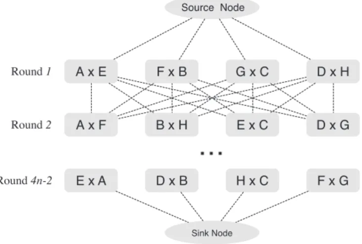
We present a ﬂow formulation for the TUP based on the formula-tions presented byTrick and Yildiz (2007)andde Oliveira et al. (2014). A graphG=

(

V,E

)

is given, in which each node represents a game and directed edges connect the nodes (games) of roundrto the nodes of roundr+1. This graphGalso contains:

• asource node,f, and directed edges connectingfto the nodes

rep-resenting games of the ﬁrst round;

• asink node,l, and directed edges connecting the nodes

represent-ing games of the last round tol.

Fig. 1presents an example of this graph for an 8-team instance. The formulation considers the following input data:

de: distance of directed edgee;

I: set of teams

{

1, . . . ,2n

}

;

H_i: set of nodes where teamiplays at home;

R: set of rounds

{

1, . . . ,4n−2

}

;

Q′

ir: set of nodes (games) of teamiplaying at home in roundsR∩

{

r, . . . ,r+q1−1

}

;

Q′′

ir: set of nodes (games) of teami(home or away) in roundsR∩

{

r, . . . ,r+q2−1

}

;

U: set of umpires

{

1, . . . ,n

}

.

And the following variables:

xeu=

1 if edgeeis selected for umpireu 0 otherwise

Finally, let

δ

(I) and

ω

(I) denote the set of edges that respectively enter and exit the nodes inI. The formulation of the problem is given byEqs. (1)–(7).

minimize e∈E

u∈U

dexeu (1)

subject to

e∈δ(j)

u∈U

xeu=1

∀

j∈V

\{

source,sink

}

(2)

e∈δ(j)

xeu−

e∈ω(j)

xeu=

₋_{1 if}_j_{is the source}

+1 ifjis the sink 0

∀

j∈V

\{

source,sink

}

,

∀

u∈U (3)

e∈δ(Hi)

xeu≥1

∀

i∈I;

∀

u∈U (4)

e∈δ(Q′

ir)

xeu≤1

∀

i∈I;

∀

r∈R;

∀

u∈U (5)

e∈δ(Q′′

ir)

xeu≤1

∀

i∈I;

∀

r∈R;

∀

u∈U (6)

xeu∈

{

0,1

} ∀

e∈E;

∀

u∈U (7)

The objective, given byEq. (1), is to minimize the total distance traveled by the umpires. Constraints(2)ascertain that each game is officiated by exactly one umpire. Constraints(3)are ﬂow preserva-tion constraints, and together with the graph structure ensure that every umpire officiates exactly one game per round. If an umpire is at the location of a team in roundr, the umpire must leave from the same location to go to the next location in roundr+1. This is also guaranteed by the ﬂow preservation constraints. Constraints(4)state that every umpire must visit every location at least once during the season. Constraints(5)and(6)specify that every umpire must wait

q1−1 days to revisit the same home location andq2−1 days to re-visit the same team, respectively. Finally, constraints(7)specify that the variables considered are binary.

3. Branch-and-bound

Building on the branch-and-bound procedure established byLand and Doig (1960), we introduce a specialized decomposition-based algorithm to the TUP. This algorithm considers the same graph

(3)

Round1

Round2

Round3

…

Round 4n-2

(d) (d),(e) (e) Source Node

A x E

F x B

G x C

D x H

A x F

B x H

E x C

D x G

A x D

B x G

C x H

E x F

E x A

D x B

H x C

F x G

Sink Node

Umpire 1 Umpire 2 Umpire 3 Umpire 4

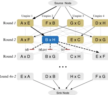
Fig. 2. Illustration of the branch-and-bound procedure for an 8-team TUP instance.

Whenever a new feasible solution is obtained, a local search pro-cedure is applied in order to improve its quality. Even if the obtained solution is not feasible, i.e. if it does not satisfy constraint (c), a lo-cal search algorithm is executed trying to ﬁrst restore feasibility and then to improve the quality of the resulting solution. The local search procedure is detailed inSection 3.4.

Fig. 2presents an example of the branch-and-bound execution in an instance with 8 teams,q1=3 andq2=2. It shows that the branch-and-bound search is currently deciding which game Umpire 1 will of-ﬁciate after game B×H. The games A×D, B×G and C×H are cut from the search tree in the current stage, as they would lead to infea-sible solutions. The ﬁrst two games would violate constraint (d) while the second and third would violate constraint (e). Thus, the only op-tion for Umpire 1 in the next round is to officiate game E×F.

3.1. Symmetry breaking

In order to speed up the branch-and-bound algorithm, we fix the games assigned to the umpires in the first round (Yildiz, 2008). This reduces symmetry in the original problem, as otherwise the umpires would be identical and introduce redundant subtrees. This preallo-cation can also be achieved by adding constraints(8)to formula-tion(1)–(7). NotationH(k) represents the edge connecting the source node to thekth game in the first round, with the games in lexico-graphic order.

xeu=1

∀

u∈U, e=H

(

u

)

(8)

3.2. Preprocessing the graph

Another way to speed up the branch-and-bound is achieved by re-moving edges that always violate one of the constraints (de Oliveira et al., 2014). Ifq1>1, then all edges connecting games in the same venue are removed. Likewise, ifq2>1 then edges connecting games of the same team are also removed. For instance, the edges connect-ing games B×H to B×G and B×H to C×H inFig. 2would be removed by this preprocessing procedure.

3.3. Additional pruning rules

Constraint (c) – every umpire should visit the home of every team at least once – can be used as an additional pruning rule, even though

it can only be evaluated on complete schedules. If the number of un-visited home locations for an umpire in a certain round exceeds the remaining number of rounds, given the assignments in the previous rounds, it is impossible to obtain a solution satisfying constraint (c). The branch-and-bound algorithm should backtrack and explore other assignments. This pruning strategy is not applied in the last round, however, because the maximum number of unvisited home locations for an umpire would be one. In this case, the local search heuristic can be used to restore feasibility, which may result in an improved upper bound.

3.4. Local search procedure

In order to quickly improve the upper bound, a local search pro-cedure is applied to the feasible and infeasible solutions obtained by the branch-and-bound. This local search, introduced byWauters et al. (2014), performs a steepest descent search with a matching neighbor-hood, i.e. moves are applied until no improvement is found.

The matching neighborhood calculates the matching for each round in the solution. In order to be able to minimize infeasibility, infeasible assignments are also added to the matching problems in-curring an additional cost. For every umpireuand every gamegin a given roundr, the matching costCugfor assigning gamegto umpire

uis a combination of two deltas presented byEq. (9):

Cug=

dug+

ρ

v

_ug ₍₉₎

where

dugis the difference between the distance of the new and the current assignment,

v

_ugis the difference between the number of

hard constraint violations in the new and the current assignment, and

ρ

is a high penalty value for the violations, i.e.

ρ

is a value sufficiently large such that any variation on

v

_ugis more signiﬁcant than any

possible value for

dug.

3.5. General branch-and-bound procedure

The pseudo-code of a recursive version of the branch-and-bound algorithm is presented inAlgorithm 1. This algorithm should initially be executed as BranchBound(∅, 1, 1), i.e., receiving the parameters: (i) an empty solution, (ii) the ﬁrst umpire and (iii) the ﬁrst round. Ini-tially, the umpire and round to be analyzed in the next iteration are

Algorithm 1:Branch-and-bound algorithm.

LetS∗_{be a global variable representing the best solution,} initialized asS∗_{← ∅}

Input: SolutionS, umpireuand roundr BranchBound(S,u,r)

1 u+←(umodn)+1 (umpire to be analyzed in the next iteration)

2 r+←r+1 ifu=nandrotherwise (round to be analyzed in the next iteration)

3 A←sorted list of feasible allocations inSfor umpireuin roundr

4 foreacha∈Ado

5 ifallocation a cannot be prunedthen

6 S←S∪

{

a

}

7 ifS is not completethen

8 BranchBound(S,u+,r+)

9 else

10 S′←LocalSearch(S)

11 ifS∗= ∅or S′_{is better than S}∗_then

12 S∗←S′

(4)

Fig. 3.Example of a subproblem.

set (lines 1 and 2) and a sorted listAof possible allocations for um-pireuin roundris constructed (line 3). The algorithm then iterates through listA(line 4), pruning the allocation when possible (line 5) or adding it to the solution (line 6). If other allocations of the sched-ule remain unexplored, then the procedure is recursively executed for the next umpire and/or round (lines 7 and 8). Once the solution is complete (line 9), i.e. all the games have umpires assigned, the lo-cal search procedure described inSection 3.4is executed (line 10). If the resulting solutionS′is better than the best found, then it replaces the best solution (lines 11 and 12). Finally, the current allocation is removed in line 13.

4. Decomposition-based lower bounds

A good lower bound is a basic requirement for an efficient branch-and-bound minimization procedure. The branch-branch-and-bound proce-dure developed for the TUP employs a decomposition approach to quickly calculate strong lower bounds. Initially, the problem is de-composed into

|

R

|

−1 subproblems. Each of them consists of exactly two consecutive rounds, which enables calculating a lower bound per set of two subsequent rounds. Next, the decomposition is changed by iteratively increasing the size of the subproblems by one round. This section details this procedure, presents a simple lower bound propagation procedure and, ﬁnally, shows how the obtained lower bounds are used to reduce the search tree of the branch-and-bound procedure.

4.1. Initial lower bounds

The first subproblems contain exactly two rounds and consist of finding a set of trips (edges) for the umpires to officiate the games in these rounds. The objective thus is to find a feasible edge set that connects the subproblem’s rounds. This subproblem is a sim-ple assignment problem, and can be solved efficiently with the Hun-garian Algorithm (Munkres, 1957). Constraint

(

c

)

is ignored in the subproblems.

Fig. 3 shows an example of a subproblem with two rounds,r

andr+1. Four games are to be officiated by four umpires in each round. The solution is a matching. Note that edges violating con-straints

(

d

)

and

(

e

)

were removed from the graph. The preprocessing

procedure presented inSection 3.2avoids analyzing these infeasible connections.

The sum of the distances of all

|

R

|

−1 matchings is a valid lower bound for the problem. It is equal to the minimum-cost ﬂow with node capacity (equal to 1) for the original problem. This network ﬂow problem is a relaxation of the TUP, obtained by removing constraints (4)–(6)from formulation(1)–(7).

The lower bound obtained is used by the branch-and-bound pro-cedure for pruning. Letmrbe the value of the matching between the consecutive roundsrandr+1. The initial lower boundsLBr1,r2for the

cost between roundsr1andr2,r1<r2, are given byEq. (10).

LBr1,r2=

r∈R,r1≤r<r2

mr (10)

4.2. Solve incremental subproblems to strengthen the lower bounds

The matchings provide valid, but relatively weak lower bounds. In order to improve the quality of the bounds, we proceed by in-crementing the size of the subproblems to solve. The main idea is that subproblems with more rounds consider more constraints, thus, the obtained bounds tend to be stronger. However, by increasing the number of rounds, the subproblems become considerably harder. For instance, the subproblem with |R| rounds is equivalent to the original Traveling Umpire Problem with constraint

(

c

)

dropped.

The subproblems with three or more rounds are solved by the very same branch-and-bound presented inSection 3, except for the evalu-ation of constraint

(

c

)

,which is here irrelevant. Therefore, the prun-ing rules presented inSection 3.3are not considered.

Lower bounds computed previously are used for pruning incre-mentally larger subproblems.Fig. 4shows an example of a subprob-lem containing four rounds of an instance with 8 teams,q1=3 and

q2=2. While solving this subproblem, the bounds obtained from smaller subproblems, with two and three rounds, are used to prune the search tree. Note that the algorithm ensures that smaller sub-problems which can provide bounds are solved before the enclos-ing ‘larger’ subproblems. For instance, in the example of Fig. 4 it is guaranteed that the subproblems with rounds

{

r+2,r+3

}

and

{

r+1,r+2,r+3

}

are solved before the algorithm solves the sub-problem with rounds

{

r,r+1,r+2,r+3

}

.

4.3. Lower bounds propagation

One of the key advantages of the decomposition approach pre-sented is that the solution of one subproblem can be used to strengthen several lower bounds. Strengthening is achieved with a simple bound propagation procedure.

Consider the subproblem ofFig. 4, which includes roundsr,r+1, r+2 andr+3. The total distance of the solution of this subproblem provides a new bound,Sr,r+3. This bound can be used to improve all values ofLBr1,r2withr1≤randr2≥r+3.Eq. (11)shows how these

(5)

Algorithm 2:Lower bounds calculation algorithm.

LetSbe an

|

R

|

×

|

R

|

matrix containing the values of solutions for the subproblems

LetLBbe an

|

R

|

×

|

R

|

matrix containing the lower bounds for all pairs of rounds

CalculateLBs()

1 S←0_|_R_|×|R|

2 LB←0_|_R_|_×_|_R_|

3 foreachr∈

{|

R

|

−1, ...,1

}

do

4 S_r_,_r₊₁←value of matching between roundsrandr+1

5 foreachr2∈

{

r+1, ...,

|

R

|}

do

6 LBr,r₂←Sr,r+1+LBr+1,r₂

7 foreachk∈

{

2, ...,

|

R

|

−1

}

do

8 r←

|

R

|

−k

9 whiler≥1do

10 foreachr′∈

{

r+k−2, ...,r

} |

S_r′_,_r₊_k=0do

11 S_r′_,_r+k←value of solution of the subproblem with rounds

{

r′, ...,r+k

}

12 foreachr₁∈

{

r′_{, ...,}₁

_}

_{, r}

2∈

{

r+k, ...,

|

R

|}

do

13 LBr₁,r₂←

max

(

LBr1,r2,LBr₁,r′+Sr′,r+k+LBr+k,r₂

)

14 r←r−k

bounds can be improved. In this equation,krepresents the difference between the ﬁrst and the last round of the subproblem (k=3 in the example ofFig. 4). Note that for anyr,LBr,r=0.

LBr1,r2=max

(

LBr1,r2,LBr1,r+Sr,r+k+LBr+k,r2

)

(11)

Eq. (11)is applied to all pairs of rounds (r1,r2), withr1∈{r, …, 1} andr2∈

{

r+k, . . . ,

|

R

|}

,possibly improving several bounds.

4.4. General lower bounds calculation algorithm

Algorithm 2 presents the lower bounds calculation procedure. The algorithm begins by setting all values of the matricesSandLBto zero (lines 1 and 2). The ﬁrst for-loop (lines 3–6) calculates the initial lower bounds for all pairs of rounds using the values of the matchings between every two consecutive rounds. The next for-loop (line 7) is responsible for solving the subproblems with more than two rounds. The difference between the ﬁrst and the last round (k) of the sub-problem starts at 2 and increases till

|

R

|

−1,i.e. the subproblem size starts at 3 and increases till |R|. Line 8 specifies the first round of the current subproblem (r). The subproblems are solved in the while-loop (line 9). Some subproblems require that lower bounds are calculated beforehand. Lines 10 and 11 guarantee this requirement, by solving first subproblems starting in roundr′₌_r₊_k₋_{2 and decrementing}

till roundr′₌_r_{. To avoid recalculation, a subproblem with rounds}

{

r′, ...,r+k

}

is solved only ifSr′,r+k=0 (line 10). The new bounds are then propagated to all pairs of rounds that can beneﬁt from the im-proved values (lines 12 and 13). Finally, the ﬁrst roundrof the next subproblem is updated (line 14).

Algorithm 2is executed in parallel during the branch-and-bound procedure. Two threads are used by the ﬁnal algorithm: one to calcu-late lower bounds (Algorithm 2) and one to compute upper bounds (Algorithm 1). Note that not all instances require solving all their subproblems. Executing both algorithms sequentially could therefore lead to a considerable waste of computation time, as it would require solving all the subproblems. Tackling both lower and upper bounds in parallel avoids this situation, since the algorithm stops whenever optimality is proven, which can be achieved before all subproblems

are solved. A possible disadvantage is that the algorithm’s execu-tion is not deterministic, since informaexecu-tion is exchanged between the threads.

4.5. Pruning strategies

The branch-and-bound procedure prunes away nodes and reduces the search tree based on the calculated lower bounds. Assume that a feasible solution with costUBis given, and that the branch-and-bound is analyzing the node corresponding to the allocation of a spe-ciﬁc game to an umpire in roundr. LetLBr, |R|be the lower bound for all allocations after roundrand letCbe the sum of the distances of all the allocations in the current solution plus the distance of the allocation being analyzed. The search tree derived from the current allocation can be pruned ifC+LB_r_,_|_R_|≥UB.

This strategy, however, has one drawback. If remaining umpires are to be assigned in roundr, the number of pruning opportunities may be limited because the boundLB_r, |R|only considers allocations of rounds afterr, while allocations are pending for roundr. To deal with this drawback and further improve the pruning strategy, the fol-lowing procedure is applied:

1. A subgraph is derived containing:

• the set of games of roundr−1 of umpires not yet allocated in

roundr,

• the set of games of roundrwith allocations pending, • the edges connecting games of these two sets.

2. A matching problem on the derived subgraph is solved.

This “partial” matching provides a valuemthat can be used to improve the lower bound, allowing to prune away a branch whenever

C+LB_r_,_|_R_|+m≥UB.

Fig. 5explains this procedure. The allocation of game C×H to Umpire 2 is being considered for round 3. Note that the game E×F of round 3 was already assigned to Umpire 1. In this case, the “partial” matching problem consists of games A×F, E×C, A×D and B×G and the edges connecting these games. Letmbe the cost of the solution of this matching problem. The allocation of C×H to Umpire 2 in the current solution is ignored ifC+LB3,|R|+m≥UB,whereCis the sum

of the distances of all the allocations in the current solution plus the cost of allocating game C×H to Umpire 2 after game D×G.

It is important to note that the “partial” matching procedure adds considerable overhead to the branch-and-bound algorithm. In or-der to reduce this overhead to an acceptable level, we employ a

(6)

Table 1

Results for instances with 12 and 14 teams.

Instance CPLEX (180 minutes) Best results from the literature Branch-and-bound

LB UB Time and LB Time and UB Time Nodes |S| LB UB 12-7,2 85,267 87,509 – – – – 0.04 2.8E+06 17 86,889 12-6,3 Infeas. – – Infeas. 0.02 9.0E+05 15 Infeas. 12-5,3 89,852 93,679 – – – – 0.02 6.3E+05 22 93,679

12-4,3 88,282 89,975 – – – – 0.09 5.5E+06 13 89,826 14-8,3 150,081 175,808 – – – – 34.83 4.9E+09 24 172,177 14-8,2 143,230 158,108 – – – – 2.92 3.5E+08 18 147,824 14-7,3 149,503 173,047 180.0 159,797 180.0 164,440 3.81 5.1E+08 26 164,440 14-7,2 142,970 152,195 – – – – 0.48 4.9E+07 25 146,656 14-6,3 149,571 166,791 2880.0 157,084 180.0 159,505 0.86 8.9E+07 26 158,875 14-6,2 143,153 145,881 – – – – 0.33 3.1E+07 26 145,124

14-5,3 149,889 162,135 2085.8 2085.8 154,962 2.17 2.0E+08 26 154,962 14-5,2 143,357 – – – – 0.18 1.5E+07 25 143,357 14A-8,3 141,233 173,475 – – – – 20.32 2.8E+09 26 166,184 14A-8,2 136,570 154,309 – – – – 2.47 2.8E+08 25 143,043 14A-7,3 141,702 167,110 180.0 153,199 180.0 158,760 2.05 2.6E+08 26 158,760 14A-7,2 136,982 148,121 – – – – 0.53 5.4E+07 25 140,562

14A-6,3 141,763 165,409 2880.0 151,044 180.0 153,216 0.50 5.5E+07 26 152,981 14A-6,2 137,497 142,892 – – – – 0.10 8.1E+06 26 138,927 14A-5,3 142,256 163,136 684.7 684.7 149,331 1.12 1.2E+08 26 149,331 14A-5,2 137,362 137,907 – – – – 0.57 6.0E+07 24 137,853 14B-8,3 141,526 172,196 – – – – 22.17 3.0E+09 22 165,026 14B-8,2 134,754 148,468 – – – – 12.78 1.5E+09 26 141,312 14B-7,3 141,721 170,436 2880.0 152,518 180.0 157,884 4.02 5.2E+08 24 157,884

14B-7,2 134,483 146,315 – – – – 1.02 1.2E+08 26 138,998 14B-6,3 141,660 161,644 2880.0 150,942 180.0 152,740 1.72 2.2E+08 26 152,740 14B-6,2 135,775 140,892 – – – – 0.86 1.0E+08 26 138,241 14B-5,3 141,972 158,405 – – 149,455 1.05 1.2E+08 26 149,455 14B-5,2 136,069 – – – – 0.20 1.9E+07 23 136,069 14C-8,3 140,223 175,801 – – – – 14.45 2.0E+09 19 161,262 14C-8,2 134,217 150,595 – – – – 16.37 2.0E+09 21 141,015

14C-7,3 140,961 168,854 180.0 151,581 180.0 154,913 0.76 9.5E+07 22 154,913 14C-7,2 133,602 149,669 – – – – 5.49 6.5E+08 26 138,832 14C-6,3 140,490 165,965 2880.0 148,987 180.0 150,858 1.67 2.1E+08 26 150,858 14C-6,2 134,752 138,109 – – – – 0.66 7.6E+07 26 136,394 14C-5,3 141,260 158,721 2880.0 147,903 180.0 149,482 12.74 1.7E+09 26 148,349 14C-5,2 134,916 – – – – 0.55 5.7E+07 26 134,916

memoization scheme (Michie, 1968) that avoids recalculation of pre-viously solved matching problems.

5. Computational experiments

The branch-and-bound algorithm was coded in Java 8 and the experiments were executed on an Intel(R) Core(TM) i7-2600 CPU @ 3.40 gigahertz computer with 16 gigabyte of RAM memory run-ning Ubuntu Linux 12.04 LTS. In the spirit of reproducible science, the source code and all the solution ﬁles are publicly available at http://gent.cs.kuleuven.be/tup.

This section is organized as follows. First the results obtained by the presented approach are compared with the best known results from the literature (de Oliveira et al., 2014; Toffolo et al., 2014; Trick & Yildiz, 2007, 2011, 2012, 2013; Trick et al., 2012; Wauters et al., 2014; Xue et al., 2015), as well as with the results obtained using formula-tion(1)–(8). Finally, the impact of the components of the presented branch-and-bound is discussed inSection 5.2.

5.1. Results of the branch-and-bound with decomposition-based lower bounds

Table 1shows the results obtained for the benchmark instances provided byTrick and Yildiz (2007)with 12 and 14 teams. The names

of the instances are abbreviated, such that ‘12-7,2’ represents in-stance umps12 withq1=7 andq2=2. The table presents, for each instance:

• the results obtained by CPLEX using formulation(1)–(8)on the

preprocessed graph (Section 3.2): the lower (LB) and upper bounds (UB) obtained in up to 3 hours;

• the best known results: the runtime (in minutes), when available,

for obtaining the best known lower bound and the best solution, as well as the values of the best lower (LB) and upper bounds (UB), collected from different papers;

• the results obtained by the presented branch-and-bound: the

run-time (in minutes), number of explored nodes and maximum size of subproblems solved byAlgorithm 2(|S|), as well as the lower (LB) and upper bounds (UB).

The best bounds are highlighted in the table, and_{indicates that} the solution was proven to be either optimal or infeasible.

Note that we also report results for non-standard instances in Table 1, withq1>nandq2=2. We conclude fromTable 1that the branch-and-bound results clearly outperform the best known results from the literature for the 14-team instances. Before this work, only three 14-team instances had their optimal proven.Xue et al. (2015)required around 46 hours to prove optimality for two of these instances (the runtime to obtain the optimal solution for instance 14B-5,3, collected from Trick and Yildiz website,2_{is unknown). The}

(7)

Table 2

Results for instances with 16 and more teams.

Instance Best results from the literature Branch-and-bound

Time and LB Time and UB Time Nodes |S| LB UB 16-8,4 180.0 193,458 – – 232.96 3.6E+10 10 Infeas. 16-8,3 – – – – 2880.00 4.0E+11 11 162,902 189,415 16-8,2 2880.0 156,089 180.0 160,705 2880.00 3.9E+11 11 145,531 184,977 16-7,4 – – – – 276.92 3.8E+10 15 197,028 16-7,3 2880.0 160,162 180.0 168,860 404.94 5.1E+10 27 165,765 16-7,2 2880.0 149,488 180.0 153,978 1101.98 1.3E+11 30 150,433 16A-8,4 2880.0 206,142 – – 225.82 3.6E+10 10 Infeas. 16A-8,3 – – – – 2880.00 4.0E+11 11 175,590 214,512 16A-8,2 2880.0 168,275 180.0 171,882 2880.00 4.5E+11 9 160,739 – 16A-7,4 – – – – 271.15 3.9E+10 14 213,416

16A-7,3 180.0 172,964 180.0 179,960 251.69 3.1E+10 26 178,511 16A-7,2 2880.0 162,622 180.0 164,620 965.37 1.2E+11 30 163,709 16B-8,4 2880.0 215,521 – – 229.41 3.6E+10 9 Infeas. 16B-8,3 – – – – 2880.00 4.1E+11 11 178,821 217,764 16B-8,2 2880.0 170,385 180.0 180,728 2880.00 3.6E+11 10 165,737 202,897 16B-7,4 – – – – 297.37 4.3E+10 13 223,868

16B-7,3 180.0 173,023 180.0 181,565 2270.28 2.9E+11 30 180,204 16B-7,2 2880.0 164,816 180.0 170,194 2301.98 2.6E+11 26 167,190 16C-8,4 2880.0 206,369 – – 236.94 3.6E+10 10 Infeas. 16C-8,3 – – – – 2880.00 4.0E+11 11 175,435 214,993 16C-8,2 2880.0 169,698 180.0 179,939 2880.00 3.7E+11 10 164,541 204,887 16C-7,4 – – – – 335.69 4.7E+10 12 209,088 16C-7,3 2880.0 172,755 180.0 184,181 2880.00 3.4E+11 18 176,161 180,483 16C-7,2 2880.0 164,626 180.0 169,184 2258.49 2.6E+11 27 166,479 18-9,4 2880.0 213,806 – – 2880.00 3.7E+11 9 193,632 – 18-9,3 – – – – 2880.00 3.8E+11 9 186,173 262,987 18-8,4 – – – – 2880.00 3.3E+11 10 197,511 254,155 18-8,3 – – – – 2880.00 3.3E+11 11 187,335 248,302 18-7,4 – – – – 2880.00 3.1E+11 15 200,551 217,502 20-10,5 180.0 216,333 – – 2880.00 3.3E+11 8 220,907 – 22-11,5 180.0 245,518 – – 2880.00 3.1E+11 6 243,052 – 24-12,6 180.0 273,057 – – 2880.00 3.5E+10 4 250,590 – 26-13,6 180.0 312,786 – – 2880.00 2.8E+10 4 289,651 – 28-14,7 180.0 350,263 – – 2880.00 9.2E+09 3 322,208 – 30-15,7 180.0 413,103 – – 2880.00 4.1E+09 3 339,331 – 32-16,8 180.0 430,890 – – 2880.00 5.2E+09 3 369,695 –

proposed branch-and-bound with decomposition-based lower bounds is able to ﬁnd (and prove) these optimal solutions in around 4 minutes, in total. Optimality was also proven in a very small amount of time for all the other 14-team instances. The procedure required, on average, around 5 minutes to solve each instance. It is noticeable, however, that instances with higher values forq1andq2 demand more computational effort from the branch-and-bound.

Table 2 shows the results for the instances with 16 and more teams. Again,indicates that the solution was proven to be opti-mal or infeasible. The best bounds are highlighted. The time limit for these hard instances was set to 48 hours, in order to enable compar-ison with the approaches proposed byXue et al. (2015). In this table, we omit the results obtained with the mathematical formulation as they were not competitive.

We can see inTable 2that the branch-and-bound found 11 op-timal solutions for the 16-team instances, improving 8 upper bound values reported in the literature. Nevertheless, some of the results obtained are poor when compared to the best results from the liter-ature. For example, no solution was obtained for instance ‘16A-8,2’. This shows that obtaining feasible solutions for highly constrained instances can take a considerable amount of time. Without an up-per bound, the proposed algorithm behaves as a naive enumeration procedure. For the more constrained instances, even solving the sub-problems is hard. This can be noticed by the smaller size |S| of the largest subproblem solved for these instances. Therefore, despite the impressive results for the 14-team instances, the algorithm’s expo-nential time complexity is noticed when solving instances with more than 14 teams. This behavior is evident in the results for the 18-team instances, where the average gap is around 21%.

5.2. Impact of the branch-and-bound components

We present experiments to analyze the impact of some of the main components of the presented branch-and-bound algorithm. Four versions of the algorithm have been prepared:

• the complete algorithm, with all the described components;

• the algorithm without the local search procedure presented in

Section 3.4;

• the algorithm without the partial matching presented in

Section 4.5;

• and the algorithm without the bound propagation presented in

Section 4.3;

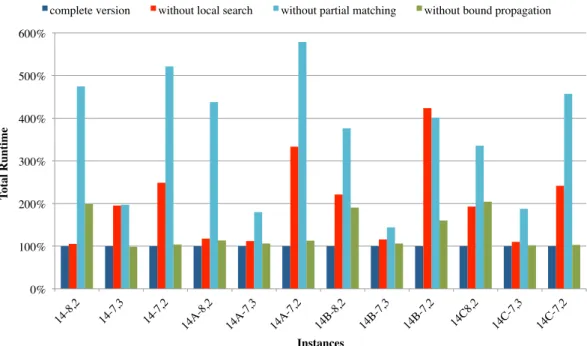
The four different versions of the algorithm were executed for the standard 14-team instances. The total runtime and the total number of nodes generated before finding (and proving) an optimal solution were analyzed.Fig. 6presents a graph showing the results of these ex-ecutions. Since the total number of nodes is proportional to the total runtime, only the runtime is shown in the figure. Therefore, the ver-tical axis presents the percentage of processing time to solve the in-stance and the horizontal axis lists the different inin-stances considered. This figure shows that removing any of the components negatively impacts the total runtime. Between the considered components, the partial matching had the highest overall impact, followed by the lo-cal search procedure. The bound propagation had the smallest impact because the subproblems could be solved very quickly.

(8)

Fig. 6. Performance of the branch-and-bound with some components deactivated on 14-team instances.

6. Conclusions and future work

This work introduced a branch-and-bound approach with decomposition-based lower bounds to the Traveling Umpire Problem, devoting attention to both computation of strong lower bounds and production of good feasible solutions.

The algorithm enabled improving a large number of lower and up-per bounds. Among these improving results, optimality was proven for all the 14-team instances and for 11 of the 16-team instances. It was also proven that no feasible solutions exist for instances ‘16-8,4’. The branch-and-bound was able to generate competitive feasible so-lutions for some of the other instances, improving the best known result in one case.

Future research can be conducted to improve the branch-and-bound in order to address larger instances. For instance, the algorithm can be parallelized and other branching rules can be investigated. The results obtained with the 18-team instances encourage this direction. It is also desirable to investigate the characteristics of the TUP that favor the performance of the presented algorithm, aiming at a gener-alized version of the procedure that can be applied to a wide range of combinatorial optimization problems.

Acknowledgments

This work was supported by the Belgian Science Policy Office (BELSPO) in the Interuniversity Attraction Pole COMEX (http://comex. ulb.ac.be) and the Leuven Mobility Research Center.

Additionally, we would like to gratefully acknowledge the anony-mous reviewers for their very helpful comments.

References

de Oliveira, L., de Souza, C. C., & Yunes, T. (2014). Improved bounds for the traveling umpire problem: a stronger formulation and a relax-and-ﬁx heuristic.European Journal of Operational Research, 236(2), 592–600.

Land, A. H., & Doig, A. G. (1960). An automatic method of solving discrete programming problems.Econometrica, 28(3), 497–520.

Michie, D. (1968). “Memo” functions and machine learning.Nature, 218, 19–22. Munkres, J. (1957). Algorithms for the assignment and transportation problems.Journal

of the Society for Industrial and Applied Mathematics, 5(1), 32–38.

Toffolo, T. A. M., Van Malderen, S., Wauters, T., & Vanden Berghe, G. (2014). Branch-and-price and improved bounds to the traveling umpire problem. InProceedings of the 10th international conference on practice and theory of automated timetabling, (PATAT, August 2014)(pp. 420–432). York, UK.

Trick, M. A., & Yildiz, H. (2007). Bender’s cuts guided large neighborhood search for the traveling umpire problem. In P. Van Hentenryck, & L. Wolsey (Eds.),Integration of AI and OR techniques in constraint programming for combinatorial optimization problems. InVolume 4510 in Lecture notes in computer science(pp. 332–345). Berlin, Heidelberg: Springer.

Trick, M. A., & Yildiz, H. (2011). Benders’ cuts guided large neighborhood search for the traveling umpire problem.Naval Research Logistics, 58(8), 771–781.

Trick, M. A., & Yildiz, H. (2012). Locally optimized crossover for the traveling umpire problem.European Journal of Operational Research, 216(2), 286–292.

Trick, M. A. Yildiz, H. (2013). Traveling umpire problem, benchmark instances.http: //mat.gsia.cmu.edu/TUP/(acessed on September 2013).

Trick, M. A., Yildiz, H., & Yunes, T. (2012). Scheduling major league baseball umpires and the traveling umpire problem.Interfaces, 42(3), 232–244.

Wauters, T., Van Malderen, S., & Vanden Berghe, G. (2014). Decomposition and local search based methods for the traveling umpire problem.European Journal of Oper-ational Research, 238(3), 886–898.

Xue, L., Luo, Z., & Lim, A. (2015). Two exact algorithms for the traveling umpire problem.

European Journal of Operational Research, 243(3), 932–943.