Dezembro de 2014
Working
Paper
374
Financial Frictions, Informality
and Income Inequality
Os artigos dos Textos para Discussão da Escola de Economia de São Paulo da Fundação Getulio Vargas são de inteira responsabilidade dos autores e não refletem necessariamente a opinião da
FGV-EESP. É permitida a reprodução total ou parcial dos artigos, desde que creditada a fonte.
Financial Frictions, Informality and Income Inequality
Giovanni Merlin
∗Vladimir K. Teles
†Abstract
We studied the effects of changes in banking spreads on distributions of income, wealth and
con-sumption as well as the welfare of the economy. This analysis was based on a model of heterogeneous
agents with incomplete markets and occupational choice, in which the informality of firms and
work-ers is a relevant transmission channel. The main finding is that reductions in spreads for firms increase
the proportion of entrepreneurs and formal workers in the economy, thereby decreasing the size of the
informal sector. The effects on inequality, however, are ambiguous and depend on wage dynamics and
government transfers. Reductions in spreads for individuals lead to a reduction in inequality
indica-tors at the expense of consumption and aggregate welfare. By calibrating the model to Brazil for the
2003-2012 period, it is possible to find results in line with the recent drop in informality and the wage
gap between formal and informal workers.
Keywords: Bank Spreads, Heterogeneous agents, Occupational Choice, Inequality,
Infor-mality.
JELs: E60, G38
1
Introduction
“Where is my bailout?” was one of the phrases on posters seen at the Occupy Wall Street movement, making clear the dissatisfaction of the population with monetary policies that tried to smooth the impact of the crisis over business cycles, but were insufficient to prevent the increase in income inequality. Under the same spirit, recent worldwide popular protests stressed that income inequality is a crucial aspect that is to be addressed by economic policies. To understand how macroeconomic policies can affect income inequality, we must understand the relationship between financial frictions and income distribution.
In this article, we study the redistributive impact of financial frictions in a model of heterogeneous agents according to Imrohoroglu (1992) and Aiyagari (1994), with imperfect markets and occupational choice. Informality, which is an important characteristic in developing countries (see Antunes & Cav-alcanti (2007)), provides a source of heterogeneity in financial friction because access to credit is more restricted for informal businesses. Given this condition, informality, inequality and credit frictions are interconnected features, and a change in spreads alters the fraction of formal and informal entrepreneurs in the economy. This, in turn, leads to a reallocation of labour demand in each sector, which changes the wage equilibrium and the proportion of workers in each sector, thus altering the distribution of consump-tion, income and wealth in the economy.
The model can be related to different studies, providing some contribution to each of them. In this context, Guerrieri & Lorenzoni (2011) analyse the effects of a credit constraint period and increased spreads on the dynamics of aggregate variables such as household consumption, interest rate and product in a model of heterogeneous agents. The authors demonstrate that an increase in the spread decreases the interest rate and the product, a result also found in the present study. However, we have focused on the redistributive impacts of interest rate variations. In this line of research, the study of Buera et al. (2012), in which the authors find that microfinance policies and credit programs targeted toward small businesses have strong impacts on income distribution, increasing welfare, particularly for less skilled and poorer agents, is relevant.
Informality has the role to include heterogeneity in terms of access to credit in our model. We can imagine several reasons for the existence of such heterogeneity, so that one can understand the informality as a metaphor for that condition to a more general understanding. Still, it is well known that informality is substantial in most countries. The literature on informality, such as Amaral & Quintin (2006); Antunes & Cavalcanti (2007); De Paula & Scheinkman (2007); Rauch (1991); Straub (2005), provides several aspects that can be incorporated in our model. In the study of Rauch (1991), for instance, formal firms are restricted to pay their employees a salary higher or equal to the minimum wage, which can lead to an excess labour supply in the formal market, which will be exploited by informal firms that face no such restriction. De Paula & Scheinkman (2007) model the informality in a manner similar to that used in this study, in which informal firms not only have more restricted access to credit but also have a probability of being detected as informal, due to the increasing “visibility” of firms represented by capital stock.
Regarding the inequality literature, perhaps the most important line of research for this study is the relative importance of transitory inequality because, in the model that will be proposed below, the agents are ex-ante identical and differ endogenously through their occupational position. The relevance of tran-sitory inequality, although usually less than that of permanent inequality, is observed in both developed countries Gustavsson (2007); Ramos (2003) and developing countries Freije & Souza (2002). Ramos (2003), for example, notes that in England during the 1990s, there was a large increase in the relevance of the transitory component of inequality, which reached 60% to 80% of inequality by the end of the decade, depending on the analysed cohort. In turn, Freije & Souza (2002) analyse the period of 1995-1997 in Venezuela and find that the transitory component represents 77% of income inequality.
fraction of workers in the informal sector decreased substantially in recent years.
The main finding is that a reduction in spreads for firms reduces informality in the economy,coeteris paribus. The impacts on inequality, however, are ambiguous and depend on the initial state of the econ-omy, the dynamics of formal wages (not incorporated in the model) and the magnitude of the cut in the spread. Whereas the gain in welfare will be higher, the stronger reduction in the spread for formal firms and the lower increase in formal wages may even be negative if the salary increase is high.
The model also demonstrates that informality, considering the current spread levels in Brazil, is ben-eficial in terms of aggregate welfare. Informality mitigates inequality because informality becomes an alternative to escape unemployment. However, in an economy without informality, the positive impacts of a reduction in the spreads for firms on inequality and welfare are higher. A reduction in spreads for individuals, if strong, benefits the informal sector and reduces inequality, despite generating welfare loss. Therefore, policies to encourage informal credit, such as microcredit, have an ambiguous effect.
The main conclusion that can be drawn from the model in terms of public policies is that the gov-ernment should encourage the reduction of the spreads for formal firms (directed or subsidised credit) and avoid high wage increases in the formal sector. Such actions would increase demand for formal employment and reduce unemployment, thus reducing inequality and increasing welfare.
2
Model
distributes the tax revenue in the form of a lump-sum transfer to all agents.
2.1
Families
We consider a unit mass of families, ex-ante identical, which maximise its intertemporal utility, given by
Ei0
" ∞
X
t=0
βtU(cit)
#
= Ei0
" ∞
X
t=0
βt
c1it−γ
1−γ
#
(1)
where β is the intertemporal discount rate, cit ∈ C ⊂ R+ refers to consumption, and γ is the risk
aversion coefficient.
In contrast to the model of Aiyagari (1994), in which the agents differ by the effective labour endow-ment, families are subject to idiosyncratic shocks regarding the quality of their business “idea”. More specifically, the individual idea, represented byθi ∈ [0,1], follows a Markov process with high
persis-tence and stationary distributionΨ(θi, θi′). 1
Process persistence is an important factor in agents remaining in the same position in the job market for a longer time. This is a reasonable hypothesis because good business ideas tend to last and remain good over time, with little probability of becoming a useless business idea in the next period.
The budget constraints of families are given bycit+sit+1 ≤ωit+ (1 +rt)(sit−eit) +eit+Tt, where
sit ∈A ⊂R+ is the savings;eit ∈A ⊂R+is the equity capital allocated to the firm, if an employer; Tt
is the lump-sum transfer by the government; andωitis the labour income. More precisely,
ωit =
wtFltF, if worker in the formal sector (FW)
wtIlIt, if worker in the informal sector (IW)
ASEθitlSEt , if self-employed worker (SE)
ΠF
it(θit, eit), if employer in the formal sector (FE)
ΠI
it(θit, eit), if employer in the informal sector (IE)
0, if unemployed (D)
(2)
where wtF(wIt) is the equilibrium wage in the formal (informal) market; lFt , lIt, lSEt are the supplied working hours; ASE is the relative productivity of self-employed workers (productivity in the formal
and informal sector production was normalised to 1); andΠF
it(ΠIit)is the profit of the formal (informal)
employer, which is a function of the idea and savings allocated to the agent’s firm i. Self-employed
1
workers are assumed to produce with constant returns to scale and labour as the only production input.2
In each period, the agents have a probabilityPF
t (PtI)of finding a job in the formal (informal) sector.
To reach a unique equilibrium with a positive work supply for both sectors, two parameters must be set:
wF
t (as in Rauch (1991)) andPtI. It is supposed thatwFt > wtI, hencePtI > PtF is a necessary condition
for inner equilibrium to occur. An implication of such an assumption is that workers with less savings will choose to work in the informal sector because the risk of not finding a job is lower in this sector. Conversely, workers with more savings may risk searching for formal jobs without having to reduce consumption drastically if a job is not found. It is noteworthy that this assumption is valid in each period, which implies that the probability of finding a job in each sector is equal to the probability of keeping one’s job in the next period. This is a strong hypothesis and is incoherent with reality 3, however, a
”search & matching”model with destruction of the job position could be incorporated into the existing model, which would make such a distinction possible but would increase the computational complexity of the problem.
Because it considers only wage differences between occupations and does not take into account wage variations within the same occupation because all formal and informal wage workers earn the same amount, the model proposed is capable of generating transitory income inequality.
2.2
Firms
Formal and informal firms are represented by an entrepreneur and produce a homogeneous good with a unit price. It is assumed that a formal firm is one that has a legal status4, pays payroll taxes,τ, and may obtain loans as a legal entity. Informal firms do not have a legal status, do not pay taxes and can incur debt only as an individual person. In addition, by operating in informality, entrepreneurs incur a quadratic cost in physical capital to avoid detection by the authorities, similar to the notion of De Paula & Scheinkman (2007), who consider an increasing probability of detection with increasing capital. The production function for both types of firm is given by a Cobb-Douglas function with decreasing returns to scale.
At the start of each period, the agents will decide the total physical capital and labour demand. They will use their own funds or intratemporal loans to acquire physical capital, which will be resold at the end
2According to the Urban Informal Economy (Economia Informal Urbana - ECINF) survey of 2003, more than 50% of
self-employed workers have no equipment or use only low-value tools/utensils.
3In general, in the formal sector, the probability of remaining in a job is expected to be greater than the probability of
finding a job, particularly in short periods of time.
4In Brazil, a firm must be registered at the Brazilian Registry of Corporate Taxpayers (Cadastro Nacional de Pessoa Jur´ıdica
of the period, discounting the depreciation value.5 6
Thus, the entrepreneuriin the periodtfaces the following restriction problem:7
maxL,D,e θitKitαLΩit−(1 +τ)wFt Lit−rtFDit−δKit−rteit, if formal
maxL,D,e θitKitαLitΩ−wItLit−rtIDit− φ2Kit2 −δKit−rteit, if informal
(3)
whereKit =Dit+eit;Dit ∈ [0,∞)is the total debt of the firm;eit ∈[0, sit]is the equity capital of
the entrepreneur, whose opportunity cost is equal tort;δis the depreciation rate of the physical capital;
andφ is the parameter related to the cost of concealing informality. It is assumed that there is no risk of becoming an employer. The first-order conditions of the problem (3) lead to the labour demand functions of the entrepreneuri:
LFit =
θiΩKitα
(1 +τ)wFt
1−1Ω
e LIit =
θiΩKitα
wIt
1−1Ω
(4)
For the choice of physical capital, the problem is restricted because the equity capital cannot be greater than the individual savings. The problem of the informal firm does not have a closed solution, and thus, it is worth analysing the marginal return on capital, which is given by the following:
RM gKit=
α
1−Ω(Dit+eit) α+Ω−1
1−Ω θ
1 1−Ω
it
h
Ω (1−τ)wFt
i1−ΩΩ
−δ, if formal
α
1−Ω(Dit+eit) α+Ω−1
1−Ω θ
1 1−Ω
it
h
Ω (1−τ)wFt
i1−ΩΩ
−φ(Dit+eit)−δ, if informal
(5)
If the marginal return on capital, evaluated as eit ≤ sit, is lower than the return rate on savings,rt,
then the entrepreneuri will not request a loan. However, if the marginal return on capital, evaluated as
sit+ε∀ε >0, is higher than the debt cost -rFou rI-, then employers will decide to incur debt.
2.3
Banking Sector
Financial intermediary agents, i.e., banks, obtain funds by means of family savings, whose remuneration isrt. To perform financial intermediation, banks incur exogenous costs,χF andχI, per capital unit lent
5For simplicity, the production sector of capital goods is not included in the model.
6Depreciation is normally present in the budget constraint of the agents, but the agents do not hold physical capital, and
only those who decide to become entrepreneurs incur this cost.
7
The entrepreneur’s profit cannot be confused with equation 2.3, as the termrteitrepresents only the opportunity cost of
to formal firms and families, respectively. It is assumed, such as in Guerrieri & Lorenzoni (2011), that the financial sector is perfectly competitive, which implies zero profit. Thus,χF andχI can be interpreted as
spreads for formal firms and families. Hence, the interest rates for loans are as follows:
(1 +rtF) = (1 +rt)(1 +χF), for formal firms
(1 +rtI) = (1 +rt)(1 +χI), for families and informal firms
(6)
Although greatly simplified, the adoption of this structure for the banking sector facilitates the analysis of the effects of spreads in other economic sectors. If some type of modification such as monopolistic competition or endogenous spreads was to be added to the model, it would be more difficult to identify the isolated effect of spreads.
2.4
Government
The public sector revenue arises from payroll taxation of the formal sector. The expenditures are lump-sum transfers to all agents,Tt, or non-productive expenditures,Gt.8 Furthermore, it is assumed that the
government restriction is active throughout the whole period, i.e., there is no public debt. Thus, the budget constraint of the government is the following:
Tt+Gt=wFt LFtτ (7)
Lump-sum transfers (which can be interpreted here, in addition to direct transfers, as the provision of public goods such as education, health and others) play an important role in the model because they provide agents with a minimum consumption level, regardless of their position in the labour market. Without transfers, the agents would choose to save more in case of unemployment.
2.5
Equilibrium
Definition: A recursive competitive stationary equilibrium consists of a value functionV :A×E →R;
a decision sequence of the agentsS′
:A×E →R,C :A×E →R+; choices of firmsKF, KI, LF, LI;
pricesr, rF, rI, wF, wI; and government policiesT:
1. Given prices and government policies, families, which are subject to their budget constraints,
max-8With the exception of the simulation performed in the last column of Table 6, the value of non-productive expenditures is
imise their value function, given by the following:
V(s, θ) = maxc,l,s′
(
c1−γ
1−γ +β
X
θ′
∈Θ
V(s′
, θ′
)Ψ(θ, θ′ )
)
(8)
2. Given prices and government policies, formal and informal entrepreneurs maximise (3).
3. The goods, labour and asset markets are in equilibrium:9
X
s,θ
c(s, θ)λ(s, θ) +Costs =X
s,θ
[YF(s, θ) +YI(s, θ) +YSE(s, θ)]λ(s, θ) (9)
X
s,θ
lF(s, θ)λ(s, θ) =X
s,θ
LF(s, θ)λ(s, θ) (10)
X
s,θ
lI(s, θ)λ(s, θ) =X
s,θ
LI(s, θ)λ(s, θ) (11)
X
s,θ
s(s, θ)λ(s, θ) =X
s,θ
[DF(s, θ) +DI(s, θ) +DF AM(s, θ)]λ(s, θ) (12)
4. The government satisfies its budget constraint (7).
5. λ(s, θ)is a stationary distribution:
λ(s′
, θ′
) = X
θ′∈Θ
X
s,s′
λ(s, θ)Ψ(θ, θ′
) (13)
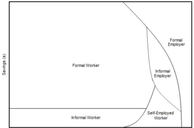
At equilibrium, for a certain set of parameters, the proportion of individuals in each of the occupational positions is constant. Figure 1 depicts how the occupational choice is made based on savings and the idea of the agents. Agents with little or no savings and without good ideas will not risk seeking a formal job because the probability of finding a position is lower than that of finding an informal job; therefore, they prefer to find a position in the informal sector. If the idea is good but not enough to be worth incurring credit loans, these agents will become self-employed workers. If they have very good ideas, they will decide to be formal employers, using the debt incurred from banks. With a certain level of savings,s∗
, the agents have enough funds to cover the risk of not finding a formal job. If they have sufficiently good ideas, they may use equity capital to run a business. When the idea is very good, entrepreneurs will prefer to become formal to have better access to credit. For lower levels of idea quality, becoming an informal
9Costs refer to the deadweight generated by depreciation and the costs of concealing informality and of financial
employer will only be worthy up to a certain degree of wealth, given the existence of the quadratic cost on capital visibility.
Figure 1: Occupational Choice
Source: Prepared by the authors.
Government transfers play an important role in determinings∗
because they provide a minimum utility level for the agents. Given the relationship between constant formal and informal wages, the higher the transfer, the lower the proportion of agents who will seek informal work.
3
Calibration and Results
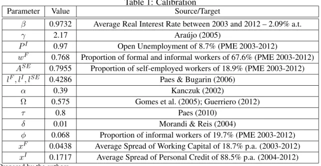
The model described in the previous section will be analysed for the Brazilian economic context by means of numerical simulations.10 It is assumed that a period of time is equivalent to one quarter. For some
parameters, values can be easily obtained from reference studies. Other parameters have been calibrated to equal the moments of some variables of interest. The calibrated values are shown in Table 1.
The discount rate, β, is selected as to obtain, in equilibrium, an annual real interest rate equivalent to 8.62% p.a., the average real interest rate in the analysed period (2003-2012)11. The value found is
0.9732. The risk aversion parameter,γ,has a value of 2.17, as estimated by Ara´ujo (2005) for Brazil. The probability of finding a job in the informal sector,PI, is calibrated as 0.97, to get closer, in equilibrium, to the average rate of open unemployment in metropolitan regions of Brazil between 2003 and 2012 of
10For simulations, values of -1 and 50 were chosen for the minimum and maximum assets that can be chosen by the
agents. The number ofgridsused was 750, which were distributed exponentially. Moreover, a margin of 1% was used for the convergence criterion. Appendix A describes the algorithm.
11The real interest rate was calculated using the SELIC as the nominal interest rate and median of inflation expectations,
Table 1: Calibration
Parameter Value Source/Target
β 0.9732 Average Real Interest Rate between 2003 and 2012 – 2.09% a.t.
γ 2.17 Ara´ujo (2005)
PI 0.97 Open Unemployment of 8.7% (PME 2003-2012)
wF 0.768 Proportion of formal and informal workers of 67.6% (PME 2003-2012) ASE 0.7955 Proportion of self-employed workers of 18.9% (PME 2003-2012) lF, lI, lSE 0.4286 Paes & Bugarin (2006)
α 0.39 Kanczuk (2002)
Ω 0.575 Gomes et al. (2005); Guerriero (2012)
τ 0.8 Paes (2010)
δ 0.01 Morandi & Reis (2004)
φ 0.068 Proportion of informal workers of 19.7% (PME 2003-2012) xF 0.0438 Average Spread of Working Capital of 18.7% p.a. (2003-2012)
xI 0.1717 Average Spread of Personal Credit of 88.5% p.a. (2004-2012)
Source: Prepared by the authors.
8.7%.12 The adopted wage of formal workers,wF, is 0.768, to approximate, in equilibrium, a proportion
of workers (formal and informal) of 67.6%, which is the average of the analysed period. The labour supply for workers,l, was calibrated as 0.4286, using as a basis the results obtained by Paes & Bugarin (2006).13
Regarding the parameters of interest for the firms, the participation of capital in the product, α, is 0.39, a value calibrated by Kanczuk (2002) and similar to other values found in literature. A value of 0.575 was chosen for the participation of labour income in the product,Ω, based on the average results of estimations made for Brazil, by Gomes et al. (2005); Guerriero (2012). Payroll tax,τ, is given a value of 0.8, as calculated by Paes (2010). The adopted depreciation rate,δ, is 0.01, a value close to that found by Morandi & Reis (2004) of 4% p.a. The quadratic cost parameter,φ, is set at 0.068 to obtain a proportion of informal workers, in equilibrium, of 19.7%, according to PME data. For the spread variablesχF andχI,
the values of 0.0438 and 0.1717, respectively, were calculated from the average values of bank spreads in credit operations for firms (working capital modality) and individuals (personal credit modality excluding consigned credit) provided by the Central Bank of Brazil.14
12Permanent and military civil servants as well as unpaid workers, who comprise approximately 8.2% of the working
population, were not considered in the analysis.
13Paes & Bugarin (2006) find an average value of 0.25 for working time over total time. Using this value, a value of 42
weekly hours is obtained. By dividing this value by the amount of available hours, which was obtained by removing 70 weekly hours from the total time for sleep and personal care, as in Guerrieri & Lorenzoni (2011), the value of 42/98 = 0.4286 is obtained.
14
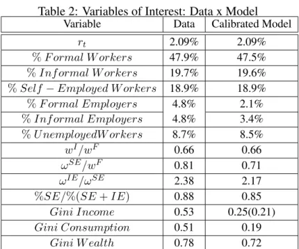
Table 2: Variables of Interest: Data x Model
Variable Data Calibrated Model
rt 2.09% 2.09%
%F ormal W orkers 47.9% 47.5%
%Inf ormal W orkers 19.7% 19.6%
%Self−Employed W orkers 18.9% 18.9%
%F ormal Employers 4.8% 2.1%
%Inf ormal Employers 4.8% 3.4%
%U nemployedW orkers 8.7% 8.5% wI/wF 0.66 0.66
ωSE/wF 0.81 0.71
ωIE/ωSE 2.38 2.17
%SE/%(SE+IE) 0.88 0.85
Gini Income 0.53 0.25(0.21) Gini Consumption 0.51 0.19
Gini W ealth 0.78 0.72
Source: Real Interest Rate (Central Bank of Brazil); Proportion of workers and wages (PME 2003-2012); Proportion of self-employed workers and informal/self-employment ratio (ECINF 2003); Gini Consumption (Silveira Neto & Menezes (2010), 2003 data); Gini Wealth (Davies et al. (2011), 2000 data).
3.1
Stationary State
Table 2 shows the moments observed in the data and those obtained in the model with the abovementioned calibration. In addition to the variables used as targets, the calibrated model is able to adequately replicate several indicators of the Brazilian economy.
The high wealth inequality obtained by the model, 0.72, is close to the observed value, 0.78. By contrast, income inequality is well below the observed inequality, a result that was expected because inequality arising from the model is mainly transitory. The labour income inequality obtained by the model is 0.25, while total income inequality (labour income + capital income + transfers) is lower due to government transfers, with a value of 0.21. The model can also adequately replicate the proportion of self-employed workers over the proportion of informal (self-employed + informal entrepreneur) “en-trepreneurs”, resulting in a value of 0.85, close to the observed value of 0.88. The average income of self-employed workers relative to formal workers is slightly underestimated at 71% but still above the income of informal workers, whose obtained ratio was 0.66, as observed in the data. The income ratio of informal entrepreneurs over self-employed workers, calculated to be 2.17, is close to the ratio calculated based on ECINF data for 2003.
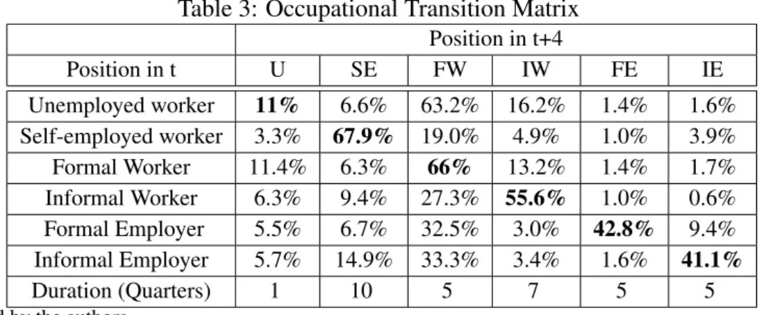
unemployment in the analysis, which would explain the higher values found. Furthermore, the model considers an equal probability of finding and continuing in the job, which increases the transition to unemployment, particularly for formal workers.
Table 3: Occupational Transition Matrix
Position in t+4
Position in t U SE FW IW FE IE
Unemployed worker 11% 6.6% 63.2% 16.2% 1.4% 1.6% Self-employed worker 3.3% 67.9% 19.0% 4.9% 1.0% 3.9% Formal Worker 11.4% 6.3% 66% 13.2% 1.4% 1.7% Informal Worker 6.3% 9.4% 27.3% 55.6% 1.0% 0.6% Formal Employer 5.5% 6.7% 32.5% 3.0% 42.8% 9.4% Informal Employer 5.7% 14.9% 33.3% 3.4% 1.6% 41.1%
Duration (Quarters) 1 10 5 7 5 5
Source: Prepared by the authors.
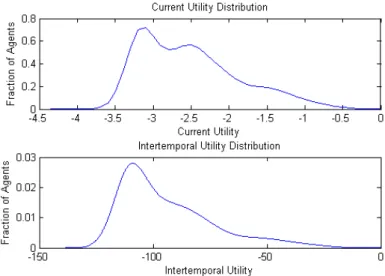
Figure 2 depicts the current and intertemporal utility value of the agents as a function of the idea and current savings. Important implications of the model can be taken from these images: i) current savings seem to be the main determinant of intertemporal utility, i.e., even if an agent with few savings has a very good idea, its intertemporal utility is far below that of an agent with more savings, regardless of his or her idea; ii) individuals with very few savings and good ideas (more specifically, in the discrete case,
θ = 0,9) decide to consume less in the current period to be able to use equity capital in their business in subsequent periods and enjoy a higher consumption level.
Figure 2: Utility as a Function of the Idea and Current Savings
Figure 3: Consumption and Income as a Function of the Idea and Current Savings
Source: Prepared by the authors.
Figure 3 illustrates the consumption and income of agents as a function of the idea and current savings. It is interesting to note that consumption practically increases linearly with savings for low idea levels but increases exponentially for agents with good ideas. This is the case because the labour income of these agents increases almost linearly with invested capital due to high returns to scale (α+ Ω = 0.965). The labour income does not depend on wealth for agents without good business ideas because the wage is equal for all workers in the formal sector.
Figure 4 shows the stationary distribution of wealth (savings) of the agents.15 It may be noted that
most agents save a small amount, only enough to smooth their consumption. The model indicates that 21% of agents have no savings, of which 15% are seeking informal work and the other 6% are self-employed workers. Hence, given a calibrated proportion of 3% of not finding a job in the informal sector, approximately 0.45% of agents consume only government transfers. Moreover, given the high interest rate for individuals, no agent chooses to obtain credit. The agents who choose to save more are the entrepreneurs, who use their funds to finance their investments in physical capital.
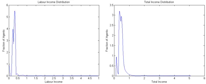
Figure 5 depicts income distributions arising from labour and total income. The distributions are multimodal. The small portion of the agents who do not have labour are the unemployed workers. The second peak includes less productive informal workers and self-employed workers. The third peak, which is basically composed of formal workers, includes more productive entrepreneurs and self-employed
15
Figure 4: Stationary Distribution of Savings
Source: Prepared by the authors.
workers.
Figure 5: Stationary Distributions of Labour Income and Total Income
Source: Prepared by the authors.
The stationary distribution of the agents’ consumption is shown in Figure 6. A multimodal distribution is also observed because consumption is dependent on income. The first peak corresponds to unemployed workers, the second comprises the mass of informal and self-employed workers, and the third peak is basically composed of the mass of formal workers. In the third peak, some more productive self-employed workers and entrepreneurs are included. Precautionary savings play an important role in consumption mitigation, with a small fraction of agents consuming only transfers.
sub-Figure 6: Stationary Distribution of Consumption
Source: Prepared by the authors.
sequent persistence in the agents’ savings. A great dispersion is observed in the distributions, which demonstrates that, even with consumption smoothing, the welfare of agents is very distinct. This re-sult is of great importance to policymakers because it affects the perception of the relationship between consumption and welfare.
3.2
Evaluation of the Brazilian Case
To evaluate the model for the Brazilian case, it is important to analyse the dynamics of the variables of interest. Figure 8 shows the evolution of bank spreads in the categories of personal credit for individuals and working capital for firms. Since 2006, there is a discrete downward trend in both spreads, which was interrupted by the temporary credit constraint caused by the financial crisis in 2008-2009, after which the downward trend intensifies. The annual average spread in the categories of personal credit and working capital decreases from 95.4% p.a. and 19.3% p.a., respectively, in 2004 to 70.7% p.a. and 13.4% p.a. in 2012.
Figure 7: Distribution of Current and Intertemporal Utility
Source: Prepared by the authors.
Figure 8: Spreads for Firms and Individuals
Table 4: Proportion of Workers in Each Labour Market Position
Unemployment Formal Worker
Informal Worker
Self-Employed
Worker
Employer
2003 12.4% 42.4% 21.0% 19.1% 5.3%
2004 11.5% 42.3% 21.8% 19.7% 5.1%
2005 9.9% 44.3% 22.0% 19.1% 5.1%
2006 10.0% 45.3% 21.3% 18.9% 4.9%
2007 9.3% 46.7% 20.5% 19.2% 4.7%
2008 7.9% 48.9% 19.8% 19.0% 4.7%
2009 8.1% 49.6% 19.1% 18.9% 4.6%
2010 6.7% 52.0% 18.4% 18.8% 4.6%
2011 6.0% 54.5% 17.2% 18.4% 4.5%
2012 5.5% 55.5% 16.4% 18.4% 4.6%
Dif. 2012 - 2003 -6.9% 13.1% -4.6% -0.8% -0.6%
Source: Monthly Employment Survey (2003-2012) - IBGE
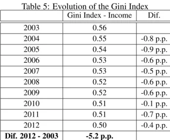
Table 5: Evolution of the Gini Index
Gini Index - Income Dif.
2003 0.56
2004 0.55 -0.8 p.p.
2005 0.54 -0.9 p.p.
2006 0.53 -0.6 p.p.
2007 0.53 -0.5 p.p.
2008 0.52 -0.6 p.p.
2009 0.52 -0.6 p.p.
2010 0.51 -0.1 p.p.
2011 0.51 -0.7 p.p.
2012 0.50 -0.4 p.p.
Dif. 2012 - 2003 -5.2 p.p.
Source: Taken from Colares (2013), calculated from data from the Monthly Employment Survey (Jan. 2003-Jul. 2012)
portion of informal workers, beginning in 2006. The proportion of self-employed workers remained relatively stable, while the proportion of employers decreased at the start of the analysed period and stabilised from 2007 onward.
3.3
Simulations
Given the dynamics of the variables analysed in the previous section, this section analyses the effects of a reduction in the spread on the proportion of agents in each occupational position and consequent al-locative and welfare effects. An analysis is performed using the spreads of 2008-2012, and the results are compared with the observed data to assess the model validity. Furthermore, counterfactual simulations are conducted, assuming a reduction of 50% in both spreads, with and without informality, and the equal-isation of spreads for individuals and spreads for firms to assess the impact of informality by isolating the effect of higher credit constraints faced by informal entrepreneurs.
3.3.1 Spread Reduction for 2008-2012 values
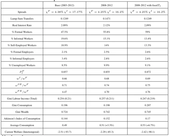
Table 6 shows the results of variables of interests for a decline in the spreads for the average values of 2008-2012. In addition, an exercise is performed in which government transfers are maintained at the same base calibration level to isolate the effect of transfers on the results.
Table 6: Spread Reduction for 2008-2012 values
Base (2003-2012) 2008-2012 2008-2012 with fixedTt
Spreads χF = 4.38%χI= 17.17% χF = 4.25%χI= 16.2% χF = 4.25%χI= 16.2%
Lump-Sum Transfers 0.1249 0.1471 0.1249
Real Interest Rate 2.09% 2.12% 2,09%
% Formal Workers 47.5% 55.8% 59%
% Informal Workers 19.6% 15.1% 13.4%
% Self-Employed Workers 18.9% 14% 13.3%
% Formal Employers 2.1% 2.5% 2.6%
% Informal Employers 3.4% 2.8% 2.6%
% Unemployed Workers 8.5% 9.9% 9.1%
PF
t 0.857 0.855 0.872
wI
/wF
0.66 0.68 0.69
ωSE/wF 0.71 0.74 0.75
ωF E
/wF
4.47 4.70 4.76
Gini Labour Income (Total) 0.254 (0.21) 0.257 (0.211) 0.247 (0.219)
Gini Consumption 0.196 0.198 0.207
Gini Wealth 0.724 0.742 0.745
Atkinson’s Index of Consumption 0.144 0.152 0.17
Average Consumption 0.49 0.51 (+3.3%) 0.53 (+6.7%)
Current Welfare (Intertemporal) -2.51 (-93.7) -2.29 (-85.3) -2.42 (-90.1)
Source: Prepared by the authors.
spreads for individuals had no effect in the analysis because, when kept at very high levels, no agent uses credit to smooth consumption or invest in informal firms. However, the reduction of spreads for formal firms increased the proportion of formal firms and the demand for physical capital, thus leading to an increase in the demand for formal work. The formal labour supply had to increase at the expense of in-formal and self-employed workers. As the wage of in-formal workers,wFt , was kept constant, formalisation occurred by increased transfers and increased savings, which decreased the risk of being unemployed, as explained in section 2.5. At equilibrium, a decrease in the wage gap occurred because the wage of infor-mal workers had to increase to equilibrate the market. Less productive self-employed workers ultimately took a risk by searching for formal jobs, thus increasing the average incomes of this category.
By keeping transfers at the same initial value, qualitatively similar results are obtained, but the effects are quantitatively stronger. An important difference is that the formal labour supply increases due to a lower probability of not finding a job, resulting in a smaller increase in unemployment, even with the strong increase in formality. Therefore, with a lower unemployment rate, labour income inequality is reduced relative to the base calibration.
Figure 9 shows the income distributions before and after the decline in spreads. Although the wage gap was reduced with the decline in spreads, the profit of formal entrepreneurs was substantially increased, and an unemployment increase was observed, which led to more people living on only transfers and capital income. Thus, inequality indicators did not decrease and changed little, as observed in Table 6. Increased inequality arising from these two effects exceeded the reduction caused by the drop in the wage differential among workers, leading to an increase in income, wealth and consumption inequality as well as an increase in Atkinson’s Index of Consumption, an inequality measure based on welfare Atkinson (1970).
Figure 9: Change in Total Income Distribution
Source: Prepared by the authors.
to increased government transfers. Figure 10 shows the difference in welfare between stationary states, as a function of current savings and idea, arising from the change in spreads. Agents with high levels of savings exhibited few changes in their welfare, while agents with few savings benefit more from increased transfers. Thus, even if the inequality indicators increase, a reduction in the spread with a consequent increase in transfers is effective for improving the quality of life of more vulnerable agents.
Figure 10: Welfare Gain
3.3.2 Spread Reduction of 50%
Given that the reduction in spreads can significantly affect occupational choice and, to a lesser extent, inequality indices, it is essential to analyse the results of a more drastic reduction in spreads. Assuming an exogenous cut of 50% in each of the considered spreads, changes can be significant, even though the spreads remain at high levels. However, to perform this analysis, it is necessary to assume a wage change in the formal sector because if wages are kept constant, the labour demand will increase such that there will not be enough workers to supply it. Workers are expected to have some type of wage transfer as a result of a decrease in spreads because the working class has bargaining power and is represented by unions. Thus, simulations were performed assuming increases in the formal of wage of 20% and 25%.16
The results are described in Table 7.
Table 7: Spread Reduction of 50%
Base (2003-2012) wF
+20% wF
+25%
Spreads χF
= 4.38%χI
= 17.17% χF
= 2.19%χI
= 8.58% χF
= 2.19%χI
= 8.58%
Lump-Sum Transfers 0.1249 0.128 (+2.5%) 0.0772 (-38.2%)
Real Interest Rate 2.09% 2.5% 2.4%
% Formal Workers 47.5% 40.2% 23.7%
% Informal Workers 19.6% 24.6% 37.3%
% Self-Employed Workers 18.9% 18.7% 25%
% Formal Employers 2.1% 1.3% 1.0%
% Informal Employers 3.4% 3.9% 5.6%
% Unemployed Workers 8.5% 11.3% 7.5%
PtF 0.857 0.793 0.789
wI
/wF
0.66 0.56 0.52
ωSE
/wF
0.71 0.59 0.54
ωF E/wF 4.47 4.59 3.15
Gini Labour Income (Total) 0.254 (0.21) 0.296 (0.238) 0.268 (0.22)
Gini Consumption 0.196 0.221 0.199
Gini Wealth 0.724 0.64 0.541
Atkinson’s Index 0.144 0.162 0.138
Average Consumption 0.493 0.554 (+12.4%) 0.431 (-12.5%)
Current Welfare (Intertemporal) -2.51 (-93.7) -2.31 (-86.1) -2.95 (-110.1)
DI
/(DI
+DF
) 0% 0.6% 1.3%
Source: Prepared by the authors.
The results in Table 7 show that the formalisation is higher and the wage gap is smaller for smaller wage increases. Consequently, transfers are also larger. For both wage increases, wealth inequality is markedly reduced. This result is due to the increase in the interest rate and the risk of becoming unemployed, which leads more vulnerable agents to save more.
For a 20% increase in wages, indicators of income inequality and consumption increase substantially given the increase in unemployment and the wage gap. Although transfers increase, the increase is in-sufficient to compensate for these two factors. Aggregate consumption and welfare, however, increase substantially. Moreover, the reduction in the spread for individuals causes some informal entrepreneurs to obtain loans, representing a total of 0.6% of total debt in the economy.
For a wage increase of 25%, informality dominates the economy. Therefore, transfers are smaller than at the base calibration. Thus, workers will migrate to the informal or self-employment sectors to avoid unemployment, which is now more costly in terms of welfare. With the decrease in unemployment rates, income and consumption inequality become closer to the values at the base calibration, and the Atkinson’s index of consumption becomes lower than the initial value. The impacts on consumption and welfare are perverse.
3.3.3 Extinction of the Informal Sector
Another interesting effect demonstrated by the model is what would occur after a reduction in spreads if there was no informal economy, keeping all other parameters constant. Thus, the same analysis as in the previous section was made, assuming a decrease of 50% in spreads and an increase in wages of 15%, 20% and 25%, with the additional assumption that informality is nonexistent. This analysis, together with the results of the previous section, illustrates the role of informality in the relationship between spreads and inequality. The results are shown in Table 8.
Table 8: Extinction of the Informal Sector – Spread Reduction of 50%
Base (2003-2012) wF
+15% wF
+20% wF
+25%
χF
4.38% 2.19% 2.19% 2.19%
χI
17.17% 8.58% 8.58% 8.58%
Lump-Sum Transfers 0.1276 0.2499 (+95.8%) 0.1581 (+23.9%) 0.0935 (-38.2%)
Real Interest Rate 2.09% 2.54% 2.4% 2.32%
% Formal Workers 48.1% 82.8% 49.9% 28.2%
% Self-Employed Workers 37.7% 2.8% 31.2% 58.8%
% Formal Employers 2.5% 2.3% 1.6% 1.1%
% Unemployed Workers 11.7% 12.1% 17.3% 11.9%
PF
t 0.805 0.873 0.743 0.704
ωSE/wF 0.68 0.76 0.58 0.50
Gini Labour Income (Total) 0.28 (0.219) 0.229 (0.213) 0.334 (0.243) 0.331 (0.243)
Gini Consumption 0.211 0.195 0.23 0.233
Gini Wealth 0.767 0.658 0.651 0.564
Atkinson Index 0.178 0.151 0.198 0.181
Average Consumption 0.491 0.829 (+69%) 0.625 (+27.4%) 0.453 (-7.6%)
Current Welfare (Inter-temporal) -2.72 (-101.6) -1.38 (-51.4) -2.2 (-81.9) -3.12 (-116.3)
Compared to the base model with informality, the proportion of formal entrepreneurs is higher (2.5%), and the interest rate is the same. Hence, the production of the formal sector is greater, and transfers are higher. Thus, more agents will risk seeking employment in the formal sector because transfers are higher and there is no option to become informal. The result is higher unemployment rates, as expected, and a reduction in the average income of self-employed workers because agents with worse ideas and few savings will not risk seeking employment in the formal sector.
The extinction of informality, however, generates losses in terms of consumption and, in particular, of aggregate welfare. In addition, all inequality indicators increase in the absence of informality because agents have more limited occupational choices.
Regarding the role of informality in the relationship between spreads and inequality, perhaps the most important result is that the effects of a reduction of 50 % in spreads on transitory inequality become more expressive in the absence of informality. The most vulnerable workers are forced to choose between risking a formal job or accepting a lower salary while self-employed. When the formal wage increases by only 15%, the demand for formal labour increases strongly, as do transfers, leading almost 95% of agents to seek formal employment, while only agents with better ideas will work as self-employed workers or start a business. The result is a large increase in aggregate consumption and welfare as well as a reduction in all inequality indicators.
For an increase of 20% in wages, even with transfers that are approximately 25% higher, the increase in unemployment to 17.3%, together with the increase in the proportion of self-employed workers without good ideas, leads to increased income and consumption inequality. The aggregate consumption and welfare, however, increase with greater intensity than in the case where informality was present. Another difference compared to the case with informality is the increase rather than decline in the proportion of formal workers.
For the simulation with an increase of 25% in wages, consumption decreases less than in the case with informality, but the income and consumption inequality indicators undergo greater increases because the unemployment rate does not decrease. This lack of decline occurs because workers do not have the option of becoming informal and thus become self-employed workers even without having good ideas.
3.3.4 Spread Equalisation
Table 9: Spread Equalisation
Base (2003-2012) Equalisation Spreads χF = 4.38%χI= 17.17% χF =χI= 4.38%
Lump-Sum Transfers 0.1249 0.0943 (-24.5%)
Real Interest Rate 2.09% 2.26%
% Formal Workers 47.5% 36%
% Informal Workers 19.6% 30.4%
% Self-Employed Workers 18.9% 20%
% Formal Employers 2.1% 1.6%
% Informal Employers 3.4% 5.3%
% Unemployed Workers 8.5% 6.6%
PF
t 0.857 0.864
wI/wF 0.66 0.68
ωSE/wF 0.71 0.69
ωF E/wF 4.47 3.98
Gini Labour Income (Total) 0.254 (0.21) 0.229 (0.202)
Gini Consumption 0.196 0.185
Gini Wealth 0.724 0.716
Atkinson’s Index 0.144 0.131
Average Consumption 0.493 0.43 (-11.9%)
Current Welfare (Inter-temporal) -2.51 (-93.7) -2.83 (-105.7)
DI/(DI+DF) 0% 3.2%
Source: Prepared by the authors.
impact of the difference in frictions, considering only the loss of efficiency by informal firms to bypass inspection. The results are shown in Table 9.
The results show that spread equalisation encourages the choice of informality by entrepreneurs, who will then represent 5.3% of the population, while the choice of formality becomes rarer, corresponding to only 1.6% of the population. Furthermore, even with cheaper credit, only 3.2% of the financial debt is in the hands of informal entrepreneurs. Hence, by using less capital, the marginal returns related to labour of informal firms are lower than those of formal firms, which, when added to the decline in the proportion of formal entrepreneurs, leads to a decrease of nearly 12% in aggregate consumption; consumption is particularly lower among formal entrepreneurs, who suffer from the increased real interest rate.
The wage gap between formal and informal workers is slightly reduced. The most efficient self-employed workers become informal entrepreneurs, and with the decrease in government revenues due to the shrinkage of the formal sector, transfers fall nearly 25%. This decrease causes agents with mediocre ideas to become self-employed workers to avoid unemployment. With the reduction in the formal sector and the increased probability of finding employment in the formal sector, the unemployment rate falls by approximately 2 percentage points (p.p.), but welfare is still markedly reduced.
are combined with the decline in the income of formal entrepreneurs, all inequality indicators decrease, particularly labour income inequality.
This analysis serves as the basis for the study of credit incentive policies for informal firms, such as microcredit lenders. The results indicate that such policies should be viewed with caution because they may promote the growth of the informal sector.
4
Conclusion
In this study, a model of heterogeneous agents was developed with occupational choice and credit fric-tions to identify how changes in bank spreads affect the distribution of income, wealth and consumption, considering the informality channel.
The main finding is that a reduction in the spreads for firms increases the demand for physical capital by formal entrepreneurs, which increases the demand for formal employment, characterised by high unemployment rates. In addition, government transfers increase, thus stimulating demand for formal labour. The net effects on unemployment, the wage gap and inequality depend on government transfers and the size of the wage increase obtained by formal workers. The reduction of the spreads for individuals at the same level as that of spreads for firms promotes informality, which in turn reduces unemployment, the wage gap and inequality indicators at the expense of aggregate consumption and welfare.
In addition, the model demonstrates that informality allows agents to smooth income, consumption and welfare. The simulations indicate that the current Brazilian economy would be worse if informality was extinguished. However, the positive effects of reductions in spreads are small compared to those of an economy without informality.
The model suggests that a reduction in spreads combined with a low wage increase would be beneficial to reduce informality and inequality as well as to increase economic welfare. Thus, the following would be appropriate government policies: i) direct or subsidised credit for productive formal firms; ii) use of increased revenues to provide public goods, unemployment insurance and direct transfers; and iii) the prevention of increases in minimum wages and wage increases in negotiations with unions.
References
Aiyagari, S. R. (1994) Uninsured idiosyncratic risk and aggregate saving.The Quarterly Journal of Economics109,
659–84.
Amaral, P. S. & E. Quintin (2006) A competitive model of the informal sector.Journal of Monetary Economics53,
1541–1553.
Antunes, A., T. Cavalcanti, & A. Villamil (2008) Computing general equilibrium models with occupational choice
and financial frictions.Journal of Mathematical Economics44, 553–568.
Antunes, A., T. Cavalcanti, & A. Villamil (2008) The effect of financial repression and enforcement on
entrepreneur-ship and economic development.Journal of Monetary Economics55, 278–297.
Antunes, A., T. Cavalcanti, & A. Villamil (2011). The effects of credit subsidies on development. .
Antunes, A., T. Cavalcanti, & A. Villamil (2013) Costly intermediation and consumption smoothing. Economic
Inquiry51, 459–472.
Antunes, A. R. & T. V. d. V. Cavalcanti (2007) Start up costs, limited enforcement, and the hidden economy.
European Economic Review51, 203–224.
Arabage, A. (2013).Os determinantes da mudan ˜A§a da desigualdade de sal´arios no setor formal do Brasil. Ph. D.
thesis, S˜ao Paulo School of Economics.
Ara´ujo, E. (2005) Avaliando trˆes especificac¸˜oes para o fator de desconto estoc´astico atrav´es da fronteira de
volatil-idade de hansen-jaganathan: um estudo emp´ırico para o brasil.Pesquisa e planejamento econˆomico35, 49–73.
Atkinson, A. B. (1970) On the measurement of inequality.Journal of Economic Theory2, 244 – 263.
Banerjee, A. V. & A. F. Newman (1993) Occupational choice and the process of development.Journal of political
economy, 274–298.
Barros, R. P., M. Carvalho, & S. Franco (2007) O papel das transferˆencias p´ublicas na queda recente da desigualdade
de renda brasileira.Desigualdade de Renda no Brasil: uma an´alise da queda recente2, 41–86.
Buera, F. J., J. P. Kaboski, & Y. Shin (2012). The macroeconomics of microfinance. . Working Paper 17905,
National Bureau of Economic Research.
Colares, B. (2013) Pol´ıca monet´aria e desigualdade: Efeito de choques de pol´ıtica monet´aria em desigualdade de
da Silva, A. F. R. E. & V. L. Pero (2008) Segmentac¸˜ao do mercado de trabalho e mobilidade de renda entre 2002 e
2007.Associac¸˜ao Nacional dos Centros de P´os-Graduac¸˜ao em Economia.
Davies, J. B., S. Sandstr¨om, A. Shorrocks, & E. N. Wolff (2011) The level and distribution of global household
wealth*.The Economic Journal121, 223–254.
De Paula, A. & J. A. Scheinkman (2007). The informal sector. . Technical report, National Bureau of Economic
Research.
dos Santos, F. S. (2013) Ascens˜ao e queda do desemprego no brasil: 1998-2012. .
Freije, S. & A. Souza (2002) Earnings dynamics and inequality in venezuela: 1995–1997.Vanderbilt University,
Department of Economics, Working Paper.
Gomes, V., M. N. Bugarin, & R. Ellery-Jr (2005) Long-run implications of the brazilian capital stock and income
estimates.Brazilian Review of Econometrics25, 67–88.
Guerrieri, V. & G. Lorenzoni (2011). Credit crises, precautionary savings, and the liquidity trap. . Working Paper
17583, National Bureau of Economic Research.
Guerriero, M. (2012) The labour share of income around the world: evidence from a panel dataset.Manchester,
University of Manchester, Institute for Development Policy and Management (IDPM).
Gustavsson, M. (2007) The 1990s rise in swedish earnings inequality–persistent or transitory?. Applied
Eco-nomics39, 25–30.
Imrohoroglu, A. (1992) The welfare cost of inflation under imperfect insurance.Journal of Economic Dynamics
and Control16, 79–91.
Kanczuk, F. (2002) Juros reais e ciclos reais brasileiros.Revista Brasileira de Economia56, 249–267.
Lucas, R. (1978) On the size distribution of business firms.The Bell Journal of Economics, 508–523.
Morandi, L. & E. Reis (2004) Estoque de capital fixo no brasil, 1950-2002.Anais do XXXII Encontro Nacional de
Economia.
Paes, N. L. (2010) Mudan ˜A§as no sistema tribut ˜A¡rio e no mercado de cr ˜A cdito e seus efeitos sobre a
informali-dade no brasil.Nova Economia20, 315–340.
Paes, N. L. & N. S. Bugarin (2006) Parˆametros tribut´arios da economia brasileira. Estudos Econˆomicos (S˜ao
Rauch, J. E. (1991) Modelling the informal sector formally.Journal of development Economics35, 33–47.
Santos, A. L. & A. P. Souza (2007) Earnings inequality in brazil: Is it permanent or transitory?.Brazilian Review
of Econometrics27, 259–284.
Schneider, F. (2002) Size and measurement of the informal economy in 110 countries. InWorkshop on Australian
National tax centre.
Silveira Neto, R. d. M. & T. A. d. Menezes (2010) Nivel e evoluc¸˜ao da desigualdade dos gastos familiares no brasil:
uma an´alise para as regi˜oes metropolitanas no per´ıodo 1996 a 2003.Estudos Econˆomicos (S˜ao Paulo)40, 341 –
372.
Soares, S. (2010) A distribuic¸˜ao dos rendimentos do trabalho ea queda da desigualdade de 1995 a 2009.mercado
de trabalho45, 35.
Straub, S. (2005) Informal sector: the credit market channel.Journal of Development Economics78, 299–321.
A
Algorithm
The algorithm for finding the equilibrium is outlined as follows:
1. The parameters are calibrated, including the minimum and maximum number of assets and the amount ofgrids.
2. From an initial value for the lump-sum transfers of the government, τ, the utility matrix of agents is calculated, considering the best occupational choice.
3. From an initial value for the value function, V(s, θ), the best choice for the agents is calculated until convergence is reached.
4. Given the convergence of the value function, the transition matrixλ(s, θ)is obtained.
5. The new government transfer is calculated and updated. The procedure is repeated from item 2 until the excess demand for labour and capital stabilises.
6. Based on the excess demand for labour and capital, new values are assigned to rt, wIt, PtF. The
Figure 11: Invariant Distribution of Ideas
Source: Prepared by the authors.
B
Markov Process of Ideas
For computational purposes, the distribution of ideas is discretised in a Markov process with 11 states. The values of the transition matrix were chosen to generate persistence in the process and obtain a proba-bility density function similar to a normal discrete distribution with a mean of 0.5 and a standard deviation of 0.2.
Ψ(θ, θ′) =
70 10 7 5 3 1.5 1 1 0.5 0.5 0.5 0.5 70 10 5 4 3 2.5 2 1.5 1 0.5 0.5 1.5 80 5 4 3 2.5 1.5 1 0.5 0.5 0.25 1 2 90 2 1.5 1 1 0.5 0.5 0.25 0.25 0.5 1 1 93 1 1 1 0.5 0.5 0.25 0.25 0.25 0.5 0.5 1 95 1 0.5 0.5 0.25 0.25 0.25 0.5 0.5 1 1 1 93 1 1 0.5 0.25 0.25 0.5 0.5 1 1 1.5 2 90 2 1 0.25 0.5 0.5 1 1.5 2.5 3 3 5 80 1.5 0.5 0.5 1 1.5 2 2.5 3 4 5 10 70 0.5 0.5 0.5 0.5 1 1 1.5 3 5 7 10 70
/100 ⇒
1 1 1 1 1 1 1 1 1 1 1
0.96 2.14 5.25 11.48 18.33 23.67 18.33 11.48 5.25 2.14 0.96 8 /100
C
Lorenz Curves
Figure 12: Lorenz Curves - Base Calibration