MODELLING AND FORECASTING THE VOLATILITY OF BRAZILIAN ASSET RETURNS: A REALIZED VARIANCE APPROACH
BYM. R. C. CARVALHO, M. A. S. FREIRE, M. C. MEDEIROS,ANDL. R. SOUZA
ABSTRACT. The goal of this paper is twofold. First, using five of the most actively traded stocks in the Brazilian financial
market, this paper shows that the normality assumption commonly used in the risk management area to describe the distri-butions of returns standardized by volatilities is not compatible with volatilities estimated by EWMA or GARCH models. In sharp contrast, when the information contained in high frequency data is used to construct the realized volatilies measures, we attain the normality of the standardized returns, giving promise of improvements in Value at Risk statistics. We also describe the distributions of volatilities of the Brazilian stocks, showing that the distributions of volatilities are nearly lognor-mal. Second, we estimate a simple linear model to the log of realized volatilities that differs from the ones in other studies. The main difference is that we do not find evidence of long memory. The estimated model is compared with commonly used alternatives in an out-of-sample experiment.
KEYWORDS. Realized volatility, high frequency data, risk analysis, volatility forecasting, GARCH models.
VERY PRELIMINARY AND INCOMPLETE.
1. INTRODUCTION
Given the fast growth of financial markets and the development of new and more complex financial instruments, there is an ever-growing need for theoretical and empirical knowledge of the volatility of financial time series. It is widely known that daily returns of financial assets, especially of stocks, are hard to predict, if not impossible, although the volatility of the returns seems to be relatively easier to forecast. Therefore, the volatility has played a central role in modern pricing and risk-management theories. There is, however, an inherent problem to the use of models that have the volatility measure taking a central role, as the conditional variance is not directly observable. The conditional variance can be estimated, among other approaches, by the (Generalized) Autoregressive Conditional Heteroskedastic – (G)ARCH – family of models proposed by Engle (1982) and Bollerslev (1986), stochastic volatility models (Taylor 1986), or the exponentially weighted moving averages (EWMA) as advocated by the Riskmetrics methodology (Morgan 1996). These approaches are heavily based on the assumption that the conditional returns of financial time series are approximately Gaussian. However, as pointed out by Bollerslev (1987), Ter¨asvirta (1996), and Carnero, Pe˜na, and Ruiz (2001), among others, this is not a compatible assumption with the estimated volatility from the above mentioned models, since the standardized returns still have excess of kurtosis.
Date: May, 24 2004.
The search for an adequate framework for the estimation and prediction of the conditional variance of financial assets returns has led us to the analysis of high-frequency intraday data. Merton (1980) already noted that the variance over a fixed interval can be estimated arbitrarily accurately by the sum of squared realizations, provided the data are available at a sufficiently high sampling frequency. More recently, Andersen and Bollerslev (1998), showed that ex-post daily foreign exchange volatility is best measured by aggregating 288 squared five-minute returns. The five-minute frequency is a trade-off between accuracy, which is theoretically optimized using the highest possible frequency, and noise due to, for example, micro-structure frictions. Ignoring the small remaining measurement error the ex-post volatility essentially becomes “observable”. Andersen and Bollerslev (1998) used this new volatility measure to evaluate the out-of-sample forecasting performance of GARCH models. This same approach was adopted by Mota and Fernandes (2004) to compare different volatility models to the index of the S˜ao Paulo stock market.
As volatility becomes “observable”, it can be modeled directly, rather than being treated as a latent variable. Recent studies, based on the theoretical results of Andersen, Bollerslev, Diebold, and Labys (2001a), Andersen, Bollerslev, Diebold, and Labys (2003), Barndorff-Nielsen and Shephard (2002a,b), and Meddahi (2002), documented the prop-erties of realized volatilities constructed form high-frequency data. For example, Andersen, Bollerslev, Diebold, and Labys (2001a) study the bilateral exchange rates between the Japanese yen (U), the Deutsche Mark (DM), and the U.S. Dollar ($), Ebens (1999) the Dow Jones index, Andersen, Bollerslev, Diebold, and Labys (2001b) the 30 stocks underlying the Dow Jones index, and Areal and Taylor (2002) the FTSE 100 index. Pong, Shackleton, Taylor, and Xu (2002) analyzed the£/$ (£is the British Pound), Li (2002) theU/$, DM/$, and£/$exchange rates, Hol and Koopman (2002) the S&P 100 index, and Martens and Zein (2002) theU/$, S&500 and Light, Sweet, and Crude Oil. Several important characteristics of the realized volatilities came out from these studies. First, the unconditional distribution of daily returns is not skewed, but it does exhibit excess kurtosis. Daily returns are not autocorrelated (except for the first order in some cases). Second, daily returns standardized by the realized variance measure are Gaussian. Third, the unconditional distributions of realized variance and volatility are distinctly non-normal and extremely right skewed. On the other hand, the natural logarithm of the volatility is close to normality. Third, the log of the realized volatility displays a high degree of (positive) autocorrelation which dies out very slowly. Fourth, realized volatility does not seem to have a unit root, but there is clear evidence of fractional integration, roughly of order 0.40.
statistics. We also describe the distributions of volatilities of the Brazilian stocks, showing that the distributions of volatilities are nearly lognormal. Second, we estimate a simple linear model to the log of realized volatilities that differs from the ones in other studies. The main difference is that we do not find evidence of long memory. The estimated model is compared with commonly used alternatives in an out-of-sample experiment.
The paper proceeds as follows. In Section 2, we briefly describe the calculation of the realized volatility. Section 3 describes the data used in the paper and carefully analyze the distribution of the standardized returns and realized volatility. In Section 4 we estimate a simple linear model to the realized volatility and an out-of-sample experiment is conducted to evaluate the forecasting performance of the estimated models. Finally, Section 5 concludes.
2. REALIZEDVARIANCE ANDREALIZEDVOLATILITY
The present section is strongly based on Oomen (2001). The term “realized variance” refers to the sum of squared intra-day returns and “realized volatility” is the squared root of the realized variance. The realized variance is an estimator for the average or integral of instantaneous variance over the interval of interest. In fact, in a continuous time framework, it has been shown by Andersen, Bollerslev, Diebold, and Labys (2001a) and Andersen, Bollerslev, Diebold, and Labys (2003) that when the return process is assumed to follow a special semi-martingale the realized variance measure can be made arbitrarily close to the integral of instantaneous variance, provided that the intra-period returns are sampled at a sufficiently high frequency. In the present context, however, the focus will be on a discrete time model.
Letpt,j denote thejth intra day-tlogarithmic price of the security under consideration andIt,j be theσ-algebra
generated by{pa,b}aa==t,b−∞=,bj=0. Under the assumption ofN equally time-spaced intradaily observations ofp(j =
1, . . . , N), the daily return is defined as:
rt=pt,N−pt−1,N, t= 1, . . . , T.
At sampling frequencyf, we can constructNf =N
f intradaily returns: rt,i=pt,if −pt,(i−1)f, i= 1, . . . , N,
wherept,0=pt−1,N.
In the following, it is assumed that the asset’s (excess) return at the daily frequency can be characterized as:
(1) rt=h1t/2εt,
consider the situation in which intradaily returns, at sampling frequencyf, are uncorrelated and can be characterized as:
(2) rt,i=h1t,i/2εt,i,
whereεt,i∼NID(0, N−1
f ).
From (2) it is clear thatrt=PNf
i=1rt,i. Then,
(3) r2t =
Nf X i=1 rt,i 2 = Nf X i=1
r2t,i+ 2 Nf−1
X
i=1
Nf
X
j=i+1
rt,irt,j,
and
(4) E£
rt2|It,0¤=E
Nf
X
i=1
r2t,i ¯ ¯ ¯ ¯ ¯
It,0
+ 2E
Nf−1
X
i=1
Nf
X
j=i+1
rt,irt,j ¯ ¯ ¯ ¯ ¯
It,0
.
Under the assumption that the intradaily returns are uncorrelated, it directly follows that
E Nf X i=1 r2 t,i ¯ ¯ ¯ ¯ ¯
It,0
=E £
r2
t|It,0¤=ht.
As a result, two unbiased estimators for the average day-treturn variance exist, namely the squared day-treturn and the sum of squared intra day-treturns. However, it can be shown that
(5) V Nf X i=1 r2 t,i ¯ ¯ ¯ ¯ ¯
It,0
= 2 Nf Nf X i=1 h2 t,i Nf < 2 Nf Nf X i=1 ht,i p Nf
=V[rt2|It,0],
since E Nf X i=1 ht,iε2 t,i 2 ¯ ¯ ¯ ¯ ¯
It,0
= 3 N2 f Nf X i=1 h2 t,i+ 2 N2 f Nf−1
X
i=1
Nf
X
j=i+1
ht,iht,j,
and
ht= 1 Nf
Nf
X
i=1
ht,i.
In words, the average daily return variance can be estimated more accurately by summing up squared intradaily returns rather than calculating the squared daily return. In addition, when returns are observed (and uncorrelated) at any arbitrary sampling frequency, it is possible to estimate the average daily variance free of measurement error as
lim Nf→∞
V Nf X i=1 r2 t,i ¯ ¯ ¯ ¯ ¯
It,0
The only (weak) requirement on the dynamics of the intradaily return variance for the above to hold is that
Nf
X
i=1
h2t,i∝Nf1+c,
where0≤c <1. Finally, note that although the daily realized variance measure employs intradaily return data, there is no need to take the (well documented) pronounced intra-day variance pattern of the return process into account. This feature of the realized variance measure contrasts sharply with popular parametric variance models which generally require the explicit modeling on intradaily regularities in return variance.
However, when the returns are correlated, the realized volatility will be a biased estimator of the daily volatility. Although, in the context of efficient markets, the finding of correlated intradaily returns may at first sight appear puzzling, it has a sensible explanation in the context of the market micro-structure literature; see Campbell, Lo, and Mackinlay (1997, Chapter 3). When the returns are sampled at higher frequencies, market microstructure may introduce some autocorrelation in the intra-day returns, thus, driving the realized variance to be a biased estimator of the daily variance. On the other hand, lower frequencies may lead to an estimator with a higher variance. The effects of micro-structure and the optimal sampling of intradaily returns have been discussed in several papers, such as, for example, Oomen (2001), Andersen, Bollerslev, Diebold, and Labys (2003), and Bandi and Russel (2003), among others.
3. THEDATA
In this paper we use data of five out of the ten major stocks from the S˜ao Paulo Stock Market (BOVESPA), namely: Bradesco (BBDC4), Embratel (EBTP4), Petrobr´as (PETR4), Telemar (TNLP4), and Vale do Rio Doce (VALE5). The data set consists of intra-day prices observed every 15-minute from 10/01/2001 to 11/30/2003 (539 daily observations). We use data from 10/01/2001 to 04/11/2003 (379 daily observations) for in-sample evaluation and the remaining for out-of-sample analysis.
TABLE1. Mean daily realized volatility.
Asset 15-minute window 30-minute window 45-minute window
Bradesco 0.0215 0.0199 0.0200
Embratel 0.0434 0.0399 0.0404
Petrobr´as 0.0200 0.0188 0.0190
Telemar 0.0228 0.0218 0.0221
Vale 0.0172 0.0159 0.0159
Notes: The table shows the average of the daily realized volatility estimated using different sampling frequencies. The estimation period is 10/01/2001 – 04/11/2003.
On the other hand, to estimate the precision of the estimator we make use of the result of Barndoff-Nielsen and Shephard (2002a)
(6)
log³PNf
i=1rt,i2 ´
−log (ht)
s
2PNf
i=1rt,i4
3³PNf
i=1rt,i2
´2
D
→N(0,1).
Table 2 shows the average size of the 95% confidence interval for the realized volatility calculated from (6). As can be observed it seems that a 15-minute frequency is the “optimal” frequency, when a bias-efficiency trade-off is considered. Thus, this will be the chosen frequency in the remaining of this paper.
TABLE 2. Mean of the confidence intervals of the daily realized volatility.
Asset 15-minute window 30-minute window 45-minute window
Bradesco 0.000871 0.001000 0.001100
Embratel 0.004800 0.005100 0.005200
Petrobr´as 0.000867 0.000967 0.001100
Telemar 0.000930 0.001100 0.001300
Vale 0.000670 0.000724 0.000787
Notes: The table shows the average of the confidence interval of the daily realized volatility estimated using different sampling frequencies. The estimation period is 10/01/2001 – 04/11/2003.
Figure 1 shows the daily returns. The dashed lines represent the out-of-sample period.
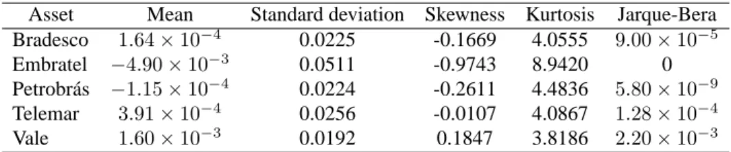
3.1. The Distribution of Standardized Returns and Realized Volatility. Table 3 shows, for each of the daily returns of the five stocks considered in this paper, the mean, the standard deviation, the skewness, the kurtosis, and thep-value of the Jarque-Bera normality test. As can be observed, as expected, all the five series have excess of kurtosis, specially Embratel. One interesting fact is that four of the series are negatively skewed, whereas Vale do Rio Doce is positive skewed. The Jarque-Bera test strongly rejects the null hypothesis of normality for all the five series.
50 100 150 200 250 300 350 400 450 500 −0.08
−0.06 −0.04 −0.02 0 0.02 0.04 0.06
Day
Return
Bradesco
(a)
50 100 150 200 250 300 350 400 450 500 −0.3
−0.25 −0.2 −0.15 −0.1 −0.05 0 0.05 0.1 0.15
Day
Return
Embratel
(b)
50 100 150 200 250 300 350 400 450 500 −0.08
−0.06 −0.04 −0.02 0 0.02 0.04 0.06
Day
Return
Petrobras
(c)
50 100 150 200 250 300 350 400 450 500 −0.08
−0.06 −0.04 −0.02 0 0.02 0.04 0.06 0.08 0.1
Day
Return
Telemar
(d)
50 100 150 200 250 300 350 400 450 500 −0.04
−0.02 0 0.02 0.04 0.06
Day
Return
Vale do Rio Doce
(e)
FIGURE1. Daily returns. The dashed lines represent the out-of-sample period. Panel (a): Bradesco. Panel (b): Embratel. Panel (c): Petrobr´as. Panel (d): Telemar. Panel (e): Vale do Rio Doce.
TABLE3. Daily returns: Descriptive statistics.
Asset Mean Standard deviation Skewness Kurtosis Jarque-Bera Bradesco 1.64×10⁻⁴ 0.0225 -0.1669 4.0555 9.00×10⁻⁵
Embratel −4.90×10⁻³ 0.0511 -0.9743 8.9420 0
Petrobr´as −1.15×10⁻⁴ 0.0224 -0.2611 4.4836 5.80×10⁻⁹ Telemar 3.91×10⁻⁴
0.0256 -0.0107 4.0867 1.28×10⁻⁴
Vale 1.60×10⁻³
0.0192 0.1847 3.8186 2.20×10⁻³ Notes: The table shows the mean, the standard deviation, the skewness, and the kurtosis of the daily returns, and thep-value of the Jarque-Bera test.
only exceptions are the GARCH(1,1), the EGARCH(1,1), and the GJR-GARCH(1,1) models estimated for Bradesco and Vale do Rio Doce and the EGARCH(1,1) and the GJR-GARCH(1,1) for Petrobr´as. Figure 2 shows the histograms of the returns and standardized returns when the daily variance is estimated by the realized volatility approach.
Table 5 shows descriptive statistics for the realized volatility. It is clear that, for all the five series, the realized volatility is strongly positively skewed and non-Gaussian. However, in accordance with the international literature, the natural logarithm of the realized volatilities are nearly Gaussian as shown in Table 6. Figures 3 and 4 show the evolution and the histogram of the realized volatility and the log realized volatility.
4. MODELLING ANDFORECASTINGREALIZEDVOLATILITY
4.1. In-sample Analysis. In order to compare the performance of different methods/models to extract the daily volatility, we estimate 95% confidence intervals for the daily returns and check the number of observations of the absolute daily returns that are greater than the interval. Table 7 shows the number of exceptions of the 95% inter-val and Table 8 shows thep-values of the tests of unconditional coverage, independence, and conditional coverage (Christoffersen 1998). All the methods/models considered in the paper seems to produce “correct” intervals.
It seems, by inspection of Figure 3 that the natural logarithm of the realized volatilities, on the contrary of the international empirical evidence, is not very persistent. Figure 5 shows the autocorrelation and partial correlation functions for the log realized volatilities. Table 9 presents the statistics and the respectivep-values of the Augmented-Dickey-Fuller (ADF) and Philipps-Perron (PP) tests for the null hypothesis of a unit-root. The unit-root hypothesis is strongly rejected for all the five series. Furthermore, there is no evidence of long-memory in the series.
Based on the evidence of no long memory in the log realized volatility series, we proceed by estimating a simple linear model for each series defined as
(7) log(ht) =α+βr2t−1+φlog(ht−1) +δlog(ht−1)×(rt−1<0) +θεt−1+ut,
where{ut}T
t=1is a sequence of independent and identically distributed random variables with zero mean and variance
σ2,ut∼IID¡ 0, σ2¢
TABLE4. Daily standardized returns: Descriptive statistics.
Asset Mean Standard deviation Skewness Kurtosis Jarque-Bera Panel I: Realized Volatility
Bradesco 0.0152 0.9956 0.0831 2.7107 0.3890
Embratel -0.0963 0.9976 0.1003 2.4461 0.0577
Petrobr´as -0.0076 1.0088 0.0122 2.4885 0.1133
Telemar 0.0236 1.0370 0.0672 2.5952 0.2177
Vale 0.1056 1.0748 0.0387 2.7161 0.4728
Panel II: EWMA (λ= 0.94)
Bradesco −7.37×10⁻⁴ 1.0334 -0.1169 3.7898 0.0061
Embratel -0.1089 1.0309 -0.4971 4.8002 6.88×10⁻¹⁵
Petrobr´as -0.0171 1.0483 -0.4817 4.7595 1.85×10⁻¹⁴
Telemar 0.0032 1.0357 -0.1474 3.7688 0.0060
Vale 0.0811 1.0312 -0.0796 4.2522 8.95×10⁻⁶
Panel II: GARCH(1,1)
Bradesco 0.0030 1.0005 -0.0757 3.5296 0.1063
Embratel 0.0067 1.0010 -0.3006 4.0334 1.80×10⁻⁵
Petrobr´as -0.0014 0.9976 -0.1800 3.5370 0.0434
Telemar -0.0064 1.0068 -0.0598 3.9023 0.0019
Vale 0.0021 0.9995 0.0180 3.5813 0.0815
Panel III: EGARCH(1,1)
Bradesco 0.0088 1.0006 -0.0365 3.5296 0.1407
Embratel -0.0008 1.0010 -0.3467 4.0334 1.43×10⁻⁷
Petrobr´as 0.0054 0.9989 -0.0989 3.5370 0.5153
Telemar -0.0069 1.0089 -0.0971 3.9023 0.0164
Vale 0.0009 0.9996 0.0292 3.5813 0.0930
Panel IV: GJR-GARCH(1,1)
Bradesco 0.0098 1.0007 -0.0343 3.4954 0.1599
Embratel 0.0053 1.0010 -0.3212 4.0521 8.98×10⁻⁶
Petrobr´as 0.0045 0.9992 -0.1131 3.2742 0.3978
Telemar -0.0059 1.0074 -0.0527 3.9142 0.0017
Vale -0.0013 0.9994 -0.0250 3.4940 0.1644
Notes: The table shows the mean, the standard deviation, the skewness, the kurtosis, and thep-value of the
Jarque-Bera test of the daily standardized returns.
TABLE5. Realized volatility: Descriptive statistics.
Asset Mean Standard deviation Skewness Kurtosis Jarque-Bera
Bradesco 0.0215 0.0079 1.7447 9.6061 0
Embratel 0.0434 0.0225 5.2217 53.4585 0
Petrobr´as 0.0200 0.0091 2.0659 9.5716 0
Telemar 0.0228 0.0079 0.7927 3.5341 3.44×10⁻¹⁰
Vale 0.0172 0.0084 2.4204 12.0763 0
Notes: The table shows the mean, the standard deviation, the skewness, the kurtosis, and thep
-value of the Jarque-Bera test of the daily realized volatilities.
TABLE6. Daily log realized volatilities: Descriptive statistics.
Asset Mean Standard deviation Skewness Kurtosis Jarque-Bera
Bradesco -3.9002 0.3451 0.0753 3.5299 0.1062
Embratel -3.2200 0.3806 0.8128 5.1035 0
Petrobr´as -3.9939 0.3929 0.4693 3.4192 2.82×10⁻⁴
Telemar -3.8394 0.3473 -0.1016 2.7485 0.414
Vale -4.1530 0.4081 0.5341 3.7153 2.87×10⁻⁶
Notes: The table shows the mean, the standard deviation, the skewness, the kurtosis, and the
p-value of the Jarque-Bera test of the daily log realized volatilities.
TABLE 7. In-sample analysis: Frequency of observations of the absolute returns that are greater than a given confidence interval.
Asset Realized Volatility EWMA (λ= 0.94) GARCH(1,1) EGARCH(1,1) GJR-GARCH(1,1) Panel I: 99% Confidence Interval
Bradesco 0.0026 0.0264 0.0185 0.0211 0.0211
Embratel 0.0026 0.0264 0.0211 0.0290 0.0211
Petrobras 0.0026 0.0158 0.0211 0.0158 0.0185
Telemar 0.0053 0.0237 0.0132 0.0185 0.0132
Vale 0.0158 0.0185 0.0185 0.0132 0.0158
Panel II: 95% Confidence Interval
Bradesco 0.0449 0.0686 0.0660 0.0765 0.0712
Embratel 0.0422 0.0660 0.0554 0.0528 0.0554
Petrobras 0.0422 0.0501 0.0554 0.0528 0.0501
Telemar 0.0528 0.0686 0.0607 0.0686 0.0660
Vale 0.0554 0.0554 0.0475 0.0501 0.0475
Panel III: 90% Confidence Interval
Bradesco 0.1029 0.0976 0.1055 0.1108 0.1029
Embratel 0.1003 0.1003 0.0923 0.0844 0.0923
Petrobras 0.1108 0.1082 0.1082 0.1055 0.1108
Telemar 0.1161 0.1108 0.0950 0.0976 0.1003
TABLE 8. In-sample analysis: p-value of the test of the null hypothesis of
cor-rect unconditional coverage, independence, and corcor-rect conditional coverage, at nominal significance level 0.05.
Asset Realized Volatility EWMA GARCH(1,1) EGARCH(1,1) GJR-GARCH(1,1) Panel I: Unconditional Coverage
99% Confidence Interval
Bradesco 0.0866 0.0078 0.1383 0.0585 0.0585
Embratel 0.0866 0.0078 0.0585 0.0025 0.0585
Petrobr´as 0.0866 0.2930 0.0585 0.2930 0.1383
Telemar 0.3098 0.0223 0.5515 0.1383 0.5515
Vale 0.2930 0.1383 0.1383 0.5515 0.2930
95% Confidence Interval
Bradesco 0.6402 0.1149 0.1731 0.0275 0.0737
Embratel 0.4755 0.1731 0.6346 0.8062 0.6346
Petrobr´as 0.4755 0.9906 0.6346 0.8062 0.9906
Telemar 0.8062 0.1149 0.3550 0.1149 0.1731
Vale 0.6346 0.6346 0.8214 0.9906 0.8214
Panel II: Independence 99% Confidence Interval
Bradesco 0.9419 0.2535 0.6073 0.5564 0.5564
Embratel 0.9419 0.4610 0.5564 0.4167 0.5564
Petrobr´as 0.9419 0.0742 0.1497 0.0742 0.1084
Telemar 0.8840 0.5076 0.7143 0.6073 0.7143
Vale 0.6600 0.6073 0.6073 0.7143 0.6600
95% Confidence Interval
Bradesco 0.2057 0.8214 0.7790 0.8684 0.9561
Embratel 0.2343 0.0510 0.7852 0.1348 0.1159
Petrobr´as 0.7005 0.8062 0.8673 0.9520 0.9616
Telemar 0.3832 0.6402 0.0490 0.1176 0.0897
Vale 0.1159 0.8214 0.9616 0.9616 0.8743
Panel III: Conditional Coverage 99% Confidence Interval
Bradesco 0.2298 0.0151 0.2921 0.1404 0.1404
Embratel 0.2298 0.0220 0.1404 0.0074 0.1404
Petrobr´as 0.2298 0.1168 0.0591 0.1168 0.0919
Telemar 0.5907 0.0590 0.7832 0.2921 0.7832
Vale 0.5222 0.2921 0.2921 0.7832 0.5222
95% Confidence Interval
Bradesco 0.4025 0.1003 0.3801 0.0868 0.2017
Embratel 0.3821 0.0841 0.7533 0.3173 0.2595
Petrobr´as 0.7200 0.1947 0.8808 0.9689 0.9988
Telemar 0.6634 0.6704 0.0940 0.0848 0.0937
−0.05 0 0.05 0 10 20 30 40 50
Bradesco − Daily Returns
−2 −1 0 1 2 3 0 5 10 15 20 25 30 35 40
Bradesco − Standardized Daily Returns
(a)
−0.30 −0.2 −0.1 0 0.1 10 20 30 40 50 60 70 80
Embratel − Daily Returns
−3 −2 −1 0 1 2 0 5 10 15 20 25 30 35
Embratel− Standardized Daily Returns
(b)
−0.05 0 0.05 0 10 20 30 40 50 60 70
Petrobras − Daily Returns
−2 0 2 0 5 10 15 20 25 30 35
Petrobras− Standardized Daily Returns
(c)
−0.05 0 0.05 0.1 0 10 20 30 40 50 60
Telemar − Daily Returns
−2 0 2 0 5 10 15 20 25 30 35 40
Telemar − Standardized Daily Returns
(d)
−0.04 −0.02 0 0.020.04 0.06 0 10 20 30 40 50 60
Vale do Rio Doce − Daily Returns
−2 0 2 0 5 10 15 20 25 30 35 40 45
Vale do Rio Doce − Standardized Daily Returns
(e)
FIGURE 2. Histograms of the daily returns and standardized daily returns. Panel (a): Bradesco. Panel (b): Embratel. Panel (c): Petrobr´as. Panel (d): Telemar. Panel (e): Vale do Rio Doce.
5. CONCLUSIONS
50 100 150 200 250 300 350 400 450 500 0.01 0.02 0.03 0.04 0.05 0.06 0.07 Day Realized Volatility Bradesco
50 100 150 200 250 300 350 400 450 500 −4.5
−4 −3.5 −3
Day
Log Realized Volatility
(a)
50 100 150 200 250 300 350 400 450 500 0.05 0.1 0.15 0.2 0.25 0.3 Embratel Day Realized Volatility
50 100 150 200 250 300 350 400 450 500 −4 −3.5 −3 −2.5 −2 −1.5 Day
Log Realized Volatility
(b)
50 100 150 200 250 300 350 400 450 500 0.01 0.02 0.03 0.04 0.05 0.06 0.07 Petrobras Day Realized Volatility
50 100 150 200 250 300 350 400 450 500 −4.5
−4 −3.5 −3
Day
Log Realized Volatility
(c)
50 100 150 200 250 300 350 400 450 500 0.01 0.015 0.02 0.025 0.03 0.035 0.04 0.045 Telemar Day Realized Volatility
50 100 150 200 250 300 350 400 450 500 −4.5
−4 −3.5 −3
Day
Log Realized Volatility
(d)
50 100 150 200 250 300 350 400 450 500 0.01 0.02 0.03 0.04 0.05 0.06 0.07
Vale do Rio Doce
Day
Realized Volatility
50 100 150 200 250 300 350 400 450 500 −5 −4.5 −4 −3.5 −3 Day
Log Realized Volatility
(e)
FIGURE 3. Daily realized volatilities. Panel (a): Bradesco. Panel (b): Embratel. Panel (c): Petrobr´as. Panel (d): Telemar. Panel (e): Vale do Rio Doce.
0 0.02 0.04 0.06 0 10 20 30 40 50 60 70
Bradesco − Realized Volatility
−4.5 −4 −3.5 −3 0 10 20 30 40 50
Bradesco − Log Realized Volatility
(a)
0 0.1 0.2 0.3 0
50 100 150
Embratel − Realized Volatility
−4 −3.5 −3 −2.5 −2 −1.5 0 10 20 30 40 50 60
Embratel − Log Realized Volatility
(b)
0 0.02 0.04 0.06 0 10 20 30 40 50 60 70
Petrobras − Realized Volatility
−5 −4.5 −4 −3.5 −3 0 5 10 15 20 25 30 35 40 45 50
Petrobras − Log Realized Volatility
(c)
0 0.01 0.02 0.03 0.04 0 5 10 15 20 25 30 35 40 45
Telemar − Realized Volatility
−4.5 −4 −3.5 −3 0 5 10 15 20 25 30 35 40
Telemar − Log Realized Volatility
(d)
0 0.02 0.04 0.06 0 10 20 30 40 50 60 70 80 90
Vale do Rio Doce − Realized Volatility
−5 −4.5 −4 −3.5 −3 0 10 20 30 40 50
Vale do Rio Doce − Log Realized Volatility
(e)
FIGURE4. Histograms of the daily realized volatilities and log daily realized volatilities. Panel (a): Bradesco. Panel (b): Embratel. Panel (c): Petrobr´as. Panel (d): Telemar. Panel (e): Vale do Rio Doce.
0 2 4 6 8 10 12 14 16 18 20 0 0.2 0.4 0.6 0.8 1 Lag Sample Autocorrelation
Sample Autocorrelation Function (ACF)
0 2 4 6 8 10 12 14 16 18 20 0 0.2 0.4 0.6 0.8 1 Lag
Sample Partial Autocorrelations
Sample Partial Autocorrelation Function
(a)
0 2 4 6 8 10 12 14 16 18 20 0 0.2 0.4 0.6 0.8 1 Lag Sample Autocorrelation
Sample Autocorrelation Function (ACF)
0 2 4 6 8 10 12 14 16 18 20 0 0.2 0.4 0.6 0.8 1 Lag
Sample Partial Autocorrelations
Sample Partial Autocorrelation Function
(b)
0 2 4 6 8 10 12 14 16 18 20 0 0.2 0.4 0.6 0.8 1 Lag Sample Autocorrelation
Sample Autocorrelation Function (ACF)
0 2 4 6 8 10 12 14 16 18 20 0 0.2 0.4 0.6 0.8 1 Lag
Sample Partial Autocorrelations
Sample Partial Autocorrelation Function
(c)
0 2 4 6 8 10 12 14 16 18 20 0 0.2 0.4 0.6 0.8 1 Lag Sample Autocorrelation
Sample Autocorrelation Function (ACF)
0 2 4 6 8 10 12 14 16 18 20 0 0.2 0.4 0.6 0.8 1 Lag
Sample Partial Autocorrelations
Sample Partial Autocorrelation Function
(d)
0 2 4 6 8 10 12 14 16 18 20 0 0.2 0.4 0.6 0.8 1 Lag Sample Autocorrelation
Sample Autocorrelation Function (ACF)
0 2 4 6 8 10 12 14 16 18 20 0 0.2 0.4 0.6 0.8 1 Lag
Sample Partial Autocorrelations
Sample Partial Autocorrelation Function
(e)
FIGURE5. Autocorrelation and partial autocorrelation functions of the log realized volatility. Panel (a): Bradesco. Panel (b): Embratel. Panel (c): Petrobr´as. Panel (d): Telemar. Panel (e): Vale do Rio Doce.
REFERENCES
ANDERSEN, T.,ANDT. BOLLERSLEV(1998): “Answering the skeptics: Yes, standard volatility models do provide accurate forecasts,”
Interna-tional Economic Review, 39, 885–905.
ANDERSEN, T., T. BOLLERSLEV, F. X. DIEBOLD,ANDP. LABYS(2000): “Market Microstructure Effects and the Estimation of Integrated
TABLE 9. In-sample
analy-sis: Unit-root tests.
Asset Dickey-Fuller Philipps-Perron Bradesco −8.77
(0) −14(0).38 Embratel −12.22
(0) −12(0).97 Petrobras −5.19
(0) −13(0).97 Telemar −6.92
(0) −14(0).29 Vale −10.16
(0) −17(0).69 Notes: The table shows thep-value of several
unit-roots test applied to the log of the realized volatilities.
TABLE10. In-sample analysis: Estimated models.
log(ht) =α+βrt2−1+φlog(ht−1) +δlog(ht−1)×(rt−1<0) +θεt−1+εt
Parameters Bradesco Embratel Petrobr´as Telemar Vale
α −1.02
(0.19)
∗∗
−2.69
(0.56)
∗∗
−1.01
(0.26)
∗∗
−1.35
(0.23)
∗∗
−1.50
(0.49)
∗∗
β 130.14
(19.83)
∗∗
17.56
(4.82)
∗∗
87.99
(27.16)
∗∗
123.89
(20.72)
∗∗
151.66
(49.71)
∗∗
φ 0.88
(0.02)
∗∗
0.59
(0.09)
∗∗
0.89
(0.03)
∗∗ 0
(0.03).84
∗∗ 0.83
(0.06)
∗∗
δ —- —- −0.01
(0.006)
∗
−0.02
(0.005)
∗∗
—-θ −0.82
(0.04)
∗∗
−0.33
(0.10)
∗∗
−0.70
(0.05)
∗∗
−0.77
(0.05)
∗∗
−0.75
(0.07)
∗∗
R2adj. 0.27 0.23 0.32 0.30 0.12
JB 0.18 0 0 0.33 0
LMSC(1) 0.12 0.48 0.88 0.32 0.08
LMSC(4) 0.45 0.87 0.84 0.85 0.06
LMARCH(1) 0.05 0.70 0.90 0.55 0.68
LMARCH(4) 0.42 0.70 0.98 0.93 0.007
(2001a): “The Distribution of Realized Exchange Rate Volatility,” Journal of the American Statistical Association, 96, 42–55. (2001b): “Exchange rate returns standardized by realized volatility are (nearly) Gaussian,” Multinational Finance Journal, forthcoming. (2003): “Modeling and Forecasting Realized Volatility,” Econometrica, 71, 579–625.
AREAL, N. M. P. C.,ANDS. J. TAYLOR(2002): “The Realized Volatility of the FTSE-100 Future Prices,” Journal of Futures Markets, 22, 627–648.
BANDI, F.,ANDJ. R. RUSSEL(2003): “Microstructure noise, realized volatility, and optimal sampling,” Working paper, Graduate School of Business, The University of Chicago.
BARNDOFF-NIELSEN, O.,ANDN. SHEPHARD(2002a): “Econometric Analysis of Realised Volatility and its Use in Estimating Stochastic
Volatility Models,” Journal of the Royal Statistical Society, Series B, 64, 253–280.
(2002b): “Estimating Quadratic Variation Using Realized Volatility,” Journal of Applied Econometrics, 17, 457–477.
BOLLERSLEV, T. (1986): “Generalized Autoregressive Conditional Heteroskedasticity,” Journal of Econometrics, 21, 307–328.
(1987): “A Conditional Heteroskedasticity Time Series Model for Speculative Prices and Rates of Return,” The Review of Economic and Statistics, 69, 542–547.
50 100 150 200 250 300 350 400 450 500 −0.1
−0.05 0 0.05 0.1
Day
Returns and 95% confidence interval
Bradesco
(a)
50 100 150 200 250 300 350 400 450 500 −0.6
−0.4 −0.2 0 0.2 0.4 0.6
Day
Returns and 95% confidence interval
Embratel
(b)
50 100 150 200 250 300 350 400 450 500 −0.1
−0.05 0 0.05 0.1
Day
Returns and 95% confidence interval
Petrobras
(c)
50 100 150 200 250 300 350 400 450 500 −0.08
−0.06 −0.04 −0.02 0 0.02 0.04 0.06 0.08 0.1
Day
Returns and 95% confidence interval
Telemar
(d)
50 100 150 200 250 300 350 400 450 500 −0.1
−0.05 0 0.05 0.1
Day
Returns and 95% confidence interval
Vale do Rio Doce
(e)
FIGURE 6. Daily returns and a 95% confidence interval computed with estimated and forecasted realized volatilities. The dashed lines represent the out-of-sample period. Panel (a): Bradesco. Panel (b): Embratel. Panel (c): Petrobr´as. Panel (d): Telemar. Panel (e): Vale do Rio Doce.
CARNERO, M. A., D. PENA˜ ,ANDE. RUIZ(2001): “Is Stochastic Volatility More Flexible Than GARCH?,” Working Paper Series in Statistics
and Econometrics 01-08, Universidad Carlos III de Madrid.
CHRISTOFFERSEN, P. F. (1998): “Evaluating interval forecasts,” International Economic Review, 39, 841–862.
TABLE11. Out-of-sample analysis: Frequency of observations of the daily absolute
re-turns are greater than a 95% confidence interval.
RV RV RV
Asset RV EWMA GARCH EGARCH GJR-GARCH + + +
(λ= 0.94) GARCH EGARCH GJR-GARCH
Panel I: 99% Confidence Interval
Bradesco 0.0187 0.0125 0 0 0 0.0063 0.0063 0.0063 Embratel 0.0187 0.0063 0.0063 0.0063 0.0063 0.0063 0.0063 0.0063 Petrobr´as 0.0250 0.0063 0 0 0 0.0063 0.0063 0.0063 Telemar 0.0187 0.0125 0.0063 0.0063 0.0063 0.0125 0.0125 0.0125 Vale 0.0437 0.0125 0 0 0 0.0125 0.0063 0.0125
Panel II: 95% Confidence Interval
Bradesco 0.0563 0.0437 0.0250 0.0125 0.0250 0.0437 0.0437 0.0375 Embratel 0.0750 0.0437 0.0187 0.0250 0.0187 0.0313 0.0313 0.0437 Petrobr´as 0.0750 0.0375 0.0313 0.0313 0.0250 0.0437 0.0375 0.0375 Telemar 0.0813 0.0437 0.0187 0.0187 0.0187 0.0563 0.0563 0.0563 Vale 0.0938 0.0813 0.0313 0.0313 0.0313 0.0563 0.0563 0.0563
Panel III: 90% Confidence Interval
Bradesco 0.1125 0.1063 0.0750 0.0563 0.0688 0.0938 0.0875 0.0875 Embratel 0.0875 0.0813 0.0500 0.0688 0.0500 0.0750 0.0680 0.0750 Petrobr´as 0.1250 0.0813 0.0563 0.0500 0.0500 0.0875 0.0813 0.0750 Telemar 0.1375 0.0938 0.0625 0.0563 0.0625 0.0875 0.0813 0.0875 Vale 0.1375 0.1187 0.0813 0.0688 0.0750 0.1250 0.1125 0.1313
ENGLE, R. F. (1982): “Autoregressive Conditional Heteroskedasticity with Estimates of the Variance of UK Inflations,” Econometrica, 50, 987– 1007.
GLOSTEN, L., R. JAGANNANTHAN,ANDR. RUNKLE(1993): “On The Relationship Between The Expected Value and The Volatility of The
Nominal Excess Returns on Stocks,” Journal of Finance, 48, 1779–1801.
HOL, E.,ANDS. J. KOOPMAN(2002): “Stock Index Volatility Forecasting with High Frequency Data,” Discussion Paper 2002-068/4, Tinbergen Institute.
LI, K. (2002): “Long Memory Versus Option-Implied Volatility Predictions,” Journal of Derivatives, 9, 9–25.
MARTENS, M.,ANDJ. ZEIN(2002): “Forecasting Financial Volatility: High-Frequency Time-Series Forecasts Vis-a-Vis Implied Volatility,”
Working paper, Erasmus University.
MEDDAHI, N. (2002): “A theoretical Comparison Between Integrated and Realized Volatility,” Journal of Applied Econometrics, 17, 479–508.
MERTON, R. C. (1980): “On Estimating the Expected Return on the Market: An Exploratory Investigation,” Journal of Financial Economics, 8,
323–361.
MORGAN, J. P. (1996): J. P. Morgan/Reuters Riskmetrics – Technical Document. J. P. Morgan, New York.
MOTA, B.,ANDM. FERNANDES(2004): “Desempenho de Estimadores de Volatilidade na Bolsa de Valores de S˜ao Paulo,” Revista Brasileira de Economia, forthcoming.
OOMEN, R. C. A. (2001): “Using High Frequency Stock Market Index Data to Calculate, Model, and Forecast Realized Return Variance,” Working Paper 2001/6, European University Institute.
PONG, S., M. B. SHACKLETON, S. J. TAYLOR,ANDX. XU(2002): “Forecasting Sterling/Dollar Volatility: Implied Volatility Versus Long Memory Intraday Models,” Working paper, Lancaster University.
TAYLOR, S. J. (1986): Modelling Financial Time Series. John Wiley.
TERASVIRTA¨ , T. (1996): “Two Stylized Facts anf the GARCH(1,1) Model,” Working Paper Series in Economics and Finance 96, Stockholm
School of Economics.
(M. R. C. Carvalho) DEPARTMENT OFECONOMICS, PONTIFICALCATHOLIC UNIVERSITY OFRIO DEJANEIRO, RIO DEJANEIRO, RJ,
BRAZIL.
E-mail address:marcelorcc@globo.com
(M. A. S. Freire) DEPARTMENT OFECONOMICS, PONTIFICALCATHOLICUNIVERSITY OFRIO DEJANEIRO, RIO DEJANEIRO, RJ, BRAZIL. E-mail address:mfreire@econ.puc-rio.br
(M. C. Medeiros – Corresponding author) DEPARTMENT OFECONOMICS, PONTIFICALCATHOLICUNIVERSITY OFRIO DEJANEIRO, RIO
DEJANEIRO, RJ, BRAZIL.
E-mail address:mcm@econ.puc-rio.br