Realized volatility: evidence from Brazil

(1)

R

EALIZED VOLATILITY

:

EVIDENCE FROM

B

RAZIL

M

arcos

V

início

W

ink

J

unior

P

edro

L

uiz

V

alls

P

ereira

Novembro

de 2012

T

Te

ex

x

to

t

os

s

p

pa

ar

r

a

D

Di

is

sc

c

us

u

s

ão

ã

o

320

C

CE

EQ

QE

EF

F

W

Wo

or

rk

k

in

i

ng

g

P

Pa

ap

pe

er

r

S

Se

e

ri

r

ie

es

s

(2)

Os artigos dos

Textos para Discussão da Escola de Economia de São Paulo da Fundação Getulio

Vargas

são de inteira responsabilidade dos autores e não refletem necessariamente a opinião da

FGV-EESP. É permitida a reprodução total ou parcial dos artigos, desde que creditada a fonte.

(3)

Realized Volatility: Evidence from Brazil

Marcos Vinício Wink Junior

Escola de Economia de São Paulo-FGV

Pedro L. Valls Pereira

y

Escola de Economia de São Paulo - FGV and CEQEF-FGV

November 4, 2012

Abstract

Using intraday data for the most actively traded stocks on the São Paulo Stock Market (BOVESPA) index, this study considers two recently developed models from the literature on the estimation and prediction of realized volatility: the Heterogeneous Autoregressive Model of Realized Volatility (HAR-RV), developed by Corsi (2009), and the Mixed Data Sampling model (MIDAS-RV), developed by Ghysels et al. (2004). Using measurements to compare in-sample and out-of-sample forecasts, better results were obtained with the MIDAS-RV model for in-sample forecasts.

The authors would like to thank one reviewer and also the participants of 2011 Encontro

Nacional de Economia (ANPEC). The second author would like to acknowledge the …nancial

support from CNPq.

(4)

For out-of-sample forecasts, however, there was no statistically signi…cant di¤erence between the models. We also found evidence that the use of realized volatility induces distributions of standardized returns that are closer to normal

Key words: Realized Volatility; HAR; MIDAS; High frequency …-nancial data.

JEL Codes: C22,C53,C58.

1 Introdução

Modeling the return volatility of stocks has been a growing area of research

in recent years. Models that estimate realized volatility based on intraday data

have been the most commonly studied. Hypotheses have emerged for these

mod-els with respect to the behavior of agents and the attempt to verify stylized facts

with respect to …nancial series. Returns standardized by the realized volatility

of …nancial assets are believed to have distributions that are close to normal,

which is relevant for the modeling of risk and the use of Value at Risk (V@R)

models. This study compares models for the estimation of realized volatility

of …ve stocks from the São Paulo Stock Market (BOVESPA). The models that

will be considered in this study are the Heterogeneous Autoregressive Model of

Realized Volatility (HAR-RV), developed by Corsi (2009), and the Mixed Data

Sampling model (MIDAS-RV), developed by Ghysels et al. (2004).

The models’ ability to …t and predict data is compared using in-sample and

(5)

the in-sample adjusted R2 _{and the mean squared errors (MSE). For}

out-of-sample comparisons, we use the out-of-out-of-sample MSE and a modi…ed

Diebold-Mariano test. This study will contribute to the literature on predicting realized

volatility with high frequency data for emerging countries, similar to the study

by Chung et al. (2008) for the Taiwan market and studies by Carvalho et al.

(2006) and Sá Mota and Fernandes (2004) for Brazil. In general, these studies

compared predictions from realized volatility models with GARCH class models.

None of these studies, however, used any form of control for the e¤ects of the

microstructure of the market. To control for this possible bias, this study uses a

M A(q)model to …lter data, as suggested by Hansen et al. (2008). In addition, this study is also the …rst to apply the MIDAS methodology to Brazilian data.

As Carvalho et al. (2006) assert, forecasting returns is di¢cult. Modeling

the volatility of returns, however, is easier and therefore generates more reliable

predictions. Thus, the literature on volatility modeling has expanded in recent

years.

Volatility modeling began with the estimation of ARCH-GARCH models and

the use of stochastic volatility models. However, as discussed in Corsi (2009),

these models su¤er from a “double weakness”. First, they do not represent

certain speci…c empirical characteristics of …nancial data1 _{and second, they tend}

to have nontrivial estimates, particularly when utilizing models of stochastic

1_{Most models are able to replicate some of the stylized facts such as: heavy tails, volatility}

clustering, high persistence, long memory, but only some models replicate the levearge e¤ect

(6)

volatility2_.

The next phase in the literature on volatility modeling was to attempt to

calculate volatility through the use of the squared daily return of a stock. Thus,

the estimation of volatility would be given from an observed variable that was

a proxy for true volatility, which is a latent variable. Andersen and Bollerslev

(1998), however, observed that the estimation of volatility through daily data

generates problems due to the large amount of noise associated with these

se-ries. Therefore, the authors suggested that intraday data would bring greater

precision to the estimation of volatility, which has become known in the

litera-ture as the calculation of realized volatility. The methods for estimating realized

volatility that will be considered in this study are the HAR-RV and the MIDAS.

The success of the HAR-RV method in estimating realized volatility is based

on modeling the behaviors of long-term memory volatility simply and e¢ciently.

This model was inspired by the Heterogeneous Markets Hypothesis and also by

asymmetry in the propagation of volatility. Corsi (2009) claims that there are

di¤erent types of agents in heterogeneous markets, that these agents are

con-tent with di¤erent prices and that these agents may therefore decide to perform

transactions at di¤erent moments. For the development of the realized volatility

estimation model, Corsi (2009) considers only the di¤erent time horizons of the

transactions as a source of heterogeneity. The evidence from Corsi (2009)

indi-cates that the performance of the out-of-sample HAR-RV model is comparable

2_{The exact estimation of the stochastic volatility model is computational intensive, however}

the estimation by quasi maximum likelihood is easy to implement using the Kalman Filter

(7)

to that of the ARFIMA model, which is much more complex for estimations and

is superior to the Autoregressive model, particularly for longer time horizons,

such as two weeks.

The literature on time series normally uses models involving samples with

identical frequencies. However, the MIDAS model developed by Ghysels et

al. (2004) considers di¤erent levels of sample frequency, which is preferable

to the normal procedure in which data are pre-…ltered and potentially useful

information may be discarded. As Ghysels et al. (2004) posit, the MIDAS model

has the advantage of a frugal estimation with a reduced number of parameters

to be estimated. As further demonstrated by Ghysels et al. (2004), the MIDAS

regressors also have desirable properties such as e¢ciency and lack of bias when

the sample tends to be more frequent.

The use of high frequency data also has a disadvantage. Anderson et al.

(2007) note that obtaining the estimator of the daily realized volatility is

bi-ased as a result of the signi…cant volume of noise associated with the market

microstructure observed in intraday data. The authors posit that this noise is

mainly associated with the fact that the prices observed are not continuous and

are quoted on a discrete grid of values. Therefore, as we will discuss below,

the observed intraday price is not a single market price at a precise instant in

time but is instead a price with market microstructure noise. Andersen et al.

(2007) discuss likely sources of market microstructure, positing that the most

frequent sources are the di¤erences between the prices for buyers and sellers

(8)

be-cause of beliefs, information, and the decision to buy or sell. To control for this

possible bias, our study uses the data …ltering process suggested by Hansen et al.

(2008). In addition, our study is also the …rst to apply the MIDAS methodology

to Brazilian data.

Following this introduction, section 2 presents the theoretical framework

on realized variance, section 3 describes the models used, section 4 provides

descriptive statistics of the data used, section 5 presents the results from the

estimations, and section 6 presents our conclusions.

2 Realized Volatility

According to McAleer and Medeiros (2008) and Andersen et al. (2003), it is

assumed that the logarithmic price processptof a particular stock in continuous

time obeys the following di¤usion:

dpt= tdWt ; t= 1;2::: (1)

wherepts the logarithm of the price over timet, tis the instantaneous

volatil-ity, strictly stationary, andWtis a standard Brownian motion. We assume that

the process described in (1) does not contain a drift component.

The sample returns withM observations per period may be calculated using

the following:

r(M);t=pt pt 1=M = 1_Z=M

0

t 1=(M+ )dWt 1=(M+ ); t= 1

M;

2

(9)

De…ning expected returns as equal to zero for any time horizon,

standard-izing the time interval byM intraday observations, and also assuming thatWt

and t are independent and conditioning the mathematical expectation in the

sample trajectory of volatility_f t+ gh=0 the return variance forhperiods may

be described as follows:

2

t;h=

h

Z

0 2

t+ d (3)

Equation [3] describes the so-called integrated variance (V I), which is a

measurement of ex-post volatility. Thus, the volatility forhperiods is identical

to the integral of past intraday volatilities. TheV I, however, is not observed

and, because it is the object of interest, it must be estimated. The intraday

return in periodmand on dayt is de…ned as follows:

rt;m=pt;m pt;m 1 form= 1; :::; M andt= 1; :::; n (4)

The daily realized variance (RV) may be de…ned as follows:

RVt= M

X

m=1

r2t;m (5)

Andersen et al. (2003) have demonstrated that, under certain conditions

involving a lack of autocorrelation of returns, the realized variance de…ned in

equation [5] is a consistent estimator of integrated variance,RVt p

!IVt.

Real-ized Volatility (RV) is the square root of the realized variance. Barndor¤-Nielsen

et al. (2002) derived the asymptotic distribution of the integrated variance

(10)

p

np 1

2IQt

(RVt IVt) d!N(0;1) (6)

whereIQt s the integrated quarticity and is de…ned by:

IQt= 1

Z

0

4₍_t_{+ )}_d ₍₇₎

Under the hypothesis of a lack of correlation of the intraday returns, IQt

may be consistently estimated by the realized quarticity, de…ned by:

RQt=

1 3

n

X

i=1

ri;t4 (8)

3 HAR-RV and MIDAS

The models considered here will be the HAR RV and M IDAS. The

HAR RV model proposed by Corsi (2009) proposes a method for estimating

volatility using di¤erent interval sizes. e(t:) is de…ned as the partial volatility

generated by certain market components. The model is proposed as an additive

cascade of partial volatilities that follows an autoregressive-type process. Three

di¤erent components of volatility generated by di¤erent time horizons are

con-sidered; more speci…cally, in this example,e(td), refers to one day,e (w)

t , refers to

one week and, e(tm), refers to one month. Let us assume that the daily return

is given by the following:

(11)

where "t N I(0;1) and (td) is the daily integrated volatility that satis…es

e(td)=e (d)

t .

The process of partial volatility e(t:)for each time scale is a function of past

realized volatility, on an identical time scale, and the expectation of partial

volatility for the subsequent period with a longer time frame. Because the

longest time scale is monthly, we have the following models:

e(tm+1)m=c(m)+ mRV (m)

t +!e

(m)

t+1m (10)

e(tw+1)w=c(w)+

(w)_RV(w)

t + (w)Et[et(m+1)m] +!e (w)

t+1w (11)

e(td+1)d=c

(d)₊ (d)_RV(d)

t + (d)Et[et(w+1)w] +!e (d)

t+1d (12)

where RVt(m); RV (w)

t and RVtd are the monthly, weekly, and daily ex-post

realized volatilities and the volatility innovationse!(tm+1)m ,!e (w)

t+1wand e! (d) t+1d are

contemporaneously and serially uncorrelated, with a mean of zero and with a

truncated distribution in the lower tail that ensures that the partial volatilities

are positive.

Through recursive substitutions of partial volatilities, the model may be

written as follows, withe(td)=e (d)

t in mind:

(d)

t+1d=c+ (d)

RVt(d)+ (w)

RVt(w)+ (m)

RVt(m)+!e (d)

t+1d (13)

(12)

(d)

t+1d=RV

(d) t+1d+!

(d)

t+1d (14)

where!(_td₊₁)_drepresents the estimation error and the measurement of latent daily

volatility.

Therefore, substituting equation (14) into (13), we …nd:

RV_t(₊₁d)_d=c+ (d)RVt(d)+ (w)RV (w)

t + (m)RV

(m)

t +!t+1d (15)

where!t+1d=!e(td+1)d ! (d) t+1d

Equation (15) therefore describes the realized volatility through a simple

autoregressive process. As used in Corsi (2009), RVt(m), corresponds to the

mean monthly volatility, as is true for the week inRVt(w).

The HAR RV model of one-day volatility may be easily extended, as

shown by Andersen et al. (2007) and by Forsberg and Ghysels (2006) forhtime

horizons, indexed intandRVt;t+h:We de…ne the realized volatility for multiple

periods as follows:

RVt;t+h= 1

h(RVt;t+1+RVt+1;t+2+:::+RVt+h 1;t+h) (16)

where RVt;t+h refers to the increase in the RV from t to t+h periods, with

h= 1;5;10;15e20,indicating, respectively, one day, one week, two weeks, three

weeks, and one month. Therefore, theHAR RV model for multiple periods

is given by the following:

RVt;t+h=c+ (d)RVt(d)+ (w)RV (w)

t + (m)RV

(m)

(13)

Corsi (2009) further suggests that the model be estimated in its logarithmic

form because of the lognormal distribution of the realized volatility. Therefore,

the estimated model in this study is described by the following equation (18):

lnRVt;t+h=c+ (d)lnRVt(d)+ (w)lnRV (w)

t + (m)lnRV

(m)

t +!t;t+h (18)

The MIDAS models with polynomial lag structures, introduced by Ghysels

et al. (2007), involve regressors with di¤erent frequencies and thus are not

autoregressive. In the MIDAS model, the dependent variable Yt has a …xed

frequency (annual, quarterly, monthly, or daily) called the reference interval.

LetXt(m) be a sample ofm intervals of time, for example, and we then have,

with annual data, thatXt(4) corresponds to the sample with quarterly data. In

this regard, a MIDAS regression is

Yt= +B(L1=m)Xt(m)+" (m)

t (19)

where B(L)is a …nite or an in…nite polynomial in the lag operator, generally

parameterized as a small set of hyper-parameters3_. _B₍_L1=m_{) =} j_Xmax

j=0

BjLj=m is

a jmax polynomial (possibly in…nite) in the operator Lj=m _and _Lj=m_X(m)

t =

X_{t j=m}(m) :The operatorLj=m_{, dtherefore, produces values of}_X(m)

t lag over j=m

periods.

Following Forsberg and Ghysels (2006) and Chung et al. (2008), we

de-veloped a particular speci…cation of the MIDAS-RV model based on the Beta

function forhtime horizons.

(14)

RVt;t+h= + 50

X

k=0

b(k; 1; 2)RVt k 1;t k+"t;t+h (20)

b(k; 1; 2) =

f(k=50; 1; 2) 50

X

j=0

f(j=50; 1; 2)

(21)

f(x; 1; 2) =

x1 1₍₁ _x₎ 2 1

( 1; 2)

(22)

where ( 1; 2)is the beta function, i.e., ( 1; 2) = (

1) (2)

( 1+ 2) andf(x; 1; 2)

is the probability density functions of the beta distribution. The beta function

de…nes the 50 weights that determine the memory of the realized volatility

process.4 _Parameters

1 and 2 determine the shape of the weight function.

The higher 2, s, the more rapidly the function declines. The parameter 1

de…nes the initial trajectory of the function; thus, if 1 >1,the function jumps

before beginning to decline. 5 _{. Because long-term memory processes generally}

depend more strongly on more recent observations, what generally occurs is

1'1 and 2>1.

4 Database

The study uses the 5 most liquid stocks traded on the BOVESPA during

the period, which are Bradesco (BBDC4), Petrobrás (PETR4), Vale (VALE5),

4_{The choose of}_k = 50_{has been suggested by Ghysels et al (2006). According to the} authors, the results obtained usingk >50the results are similar.

(15)

Telemar (TNLP4), and Usiminas (USIM5). The sample includes intraday data

for 3 di¤erent time periods, at intervals of 5, 15, and 30 minutes. The period

analyzed is from 11/01/2007 to 04/30/2010.

As discussed in McAleer and Medeiros (2008), there is a debate in the

lit-erature regarding the selection of the frequency of the intraday data. As the

frequency increases (largeM), the precision also increases, as does the

proba-bility that noise will be associated with a microstructure, such as the lack of

negotiation. Andersen et al. (2001) propose 5-minute intervals. Oomen (2002)

argues that the optimal interval frequency is 25 minutes. Giot and Laurent

(2004) observe an optimal frequency of data every 15 minutes. In the face of

this debate, we chose to use data in 5-minute, 15-minute, and 30-minute

inter-vals. Table 1 shows the number of observations for each stock in each intraday

period. There are di¤erent numbers of observations because we are using the

stock price negotiated immediately after the time period.6 _{Thus, we are}

obtain-ing the price of the …rst trade after the determined time period, and more liquid

stocks will therefore have more observations because they will be more likely to

be traded right after the end of the negotiation period.

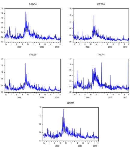
Figure 1 shows the graph of daily realized volatility using 5-minute time

intervals for each stock. An increase can be perceived in volatility in the second

6_{In general, the trade occurs in the second following the end of the negotiation period but}

(16)

half of 2008. This increased occurred because of the subprime crisis. Jumps in

volatility can also be observed for all the stocks.7

Table 2 presents the descriptive statistics of the daily returns of the 5 selected

stocks. As commonly found in the literature, the returns display an excess of

kurtosis, implying that the returns have heavy tails and therefore do not have

normal distributions, as observed in the Jarque-Bera test. It is noteworthy that

all the stocks displayed negative mean returns, primarily because the sample

covers the period of the subprime crisis.

To select the most accurate estimator of realized volatility among the

di¤er-ent frequencies, we determined the average size of the 95% con…dence interval

of the estimator, calculated from its variance described in equation (7). The

re-sults are presented in Table 3 and suggest that the smallest con…dence interval

is generated by the 5-minute frequency for all the stocks.8 _{Therefore, from this}

point onward, we will use intraday data with a 5-minute frequency.

7_{Andersen et al. (2007) state that most jumps in volatility occur due to macroeconomic}

announcements

8_{If the intraday returns were independent form the time period, the lowest-frequency}

in-terval would be the smallest-sized one; however, as they depend on time period, this result

may not be reliable. Therefore, the choice based on the lowest mean size seems to be the most

(17)

Table 4 shows the descriptive statistics of the standardized returns. Daily

volatilities were estimated by the following 5 di¤erent methods: GARCH, EGARCH,

EWMA (using the estimated decay parameter), GJR9 _{and realized volatility.}

The order of the models and the conditional distributions of the errors were

selected using the Schwarz information criterion.

The results described in Table 4 suggest that the estimation of realized

volatility induces distributions in the standardized returns that are closer to

a normal distribution in relation to the estimation of daily volatility by other

methods. This result is useful to employ in risk management through VaR

models. Another important result presented in Table 4 is the superiority of the

asymmetric models of volatility (EGARCH and GJR) compared to GARCH

models in the generation of standardized returns with normal distributions10_,

with the exception of VALE5 and TNLP4, which did not show improved results.

5 Data Filtration

As discussed above, realized variance is a consistent estimator of integrated

variance if the returns are not autocorrelated. Andersen et al. (2001), however,

show that the market microstructure generates autocorrelation of the returns.

9_{GJR model is also known as Threshold GARCH or TGARCH.}

(18)

To demonstrate this, let us assume that the observed logarithmic price of a

stockpt;iis given by the following: seja dado por:

pt;i=pt;i+"t;i (23)

where p_t;i is the latent e¢cient price and "t;i is the noise associated with the

market microstructure. The return on stockrt;i will be given by the following:

rt;i=pt;i pt;i 1=rt;i+"t;i "t;i 1 (24)

wherert;i=pt;i pt;i 1is the e¢cient return.

This shows that the noise of the microstructure generates autocorrelation

in the returns and therefore generates a biased estimation of the integrated

variance. To correct the bias caused by the market microstructure, we use

the daily realized volatility …ltered by the moving average method (…lterM A),

which was used by Ebens (1999) and Andersen et al. (2001). These authors

suggested the use of a …rst-order moving average process to model the intraday

returns of the stocks and that the …ltering would result from the use of the

residuals of this estimation. Hansen et al. (2008), however, showed that the …lter

M A(1)would be valid only under the hypothesis that the noise associated with the market microstructure is independently and identically distributed (IID);

therefore, these researchers proposed a …ltering method in which the hypothesis

of IID noise is not necessary.

Let us assume that the intraday return of a stock follows a processM A(q)

(19)

under certain conditions, for the estimation ofRV based on the processM A(q),

RVt;M A(q)is given by:

RVt;M A(q)= (1 b1 ::: bq)2 M

X

i=1

b"2t;i (25)

We have the following

E[RVt] =E

"_M X

i=1

r2t;i

#

= (1 + 21+:::+ 2q)E

2 4 M X i=1 q X j=0

"2t;i j

3

5 (26)

Because(1 b1 ::: bq)2 M

X

i=1

b"2t;i p

!IV we then have

E[RVt]

IV '

(1 + 21+:::+ 2q)

(1 1 ::: q)2

(27)

Equation (27) suggests a bias-corrected estimator for the realized variance,

g

RVt;M A(q), given by:

g

RVt;M A(q)=

(1 +e21+:::+ e 2 q)

(1 e1 ::: eq)2

RVt (28)

The estimations obtained in this study were performed from the realized

volatility …ltered by the MA(q) method described in equation (28), in which the

order of theM A was 2, selected under the information criterion

6 Results of the Estimations

In this section, we present the results of theHAR RV andM IDAS RV

(20)

described in equations (18) and (20), respectively. For both models, the realized

volatility that was used was …ltered, as per equation (28), to correct for problems

associated with the microstructure. The estimated coe¢cients of the HAR-RV

models are presented in Table 5, with their respective p-values.

Table 5 shows that the estimated coe¢cients d_; w _and m_{BLANK and}

BLANK are signi…cant, con…rming the hypothesis of the high persistence of

volatility. In addition, Table 5 shows that, on average, the estimations of d

and of w _{decline along the time horizons, as opposed to} m_{, which tends to}

be relatively more signi…cant for long-term volatility, as previously shown by

Andersen et al. (2007) and Chung et al. (2008). As in our study, Andersen

et al. (2007) did not observe a common pattern for all betas in the di¤erent

time horizons. It is noteworthy that only the PETR4 stock displayed a drop

in the estimations of d _and w_{and an increase in the estimations of BLANK,}

according to the increase in the forecast horizon for all estimations.

The estimated coe¢cients for the MIDAS-RV models are presented in Table

6 with their respective p-values.

The results described in Table 6 demonstrate that all estimated coe¢cients

di¤er signi…cantly from zero. The main parameter of interest is because

(21)

volatilities. This coe¢cient proved to be signi…cant for all stocks and for all

forecast horizons. As discussed above, the parameters 1and 2 determine the

shape of the weight function.

As expected, 1is close to 1 in all the estimations, indicating that the weight

functions decline from the …rst lag. The parameter 2 indicates the velocity of

the decline of the weight function. Because the estimated values for 2 are

relatively high, the weight function of the realized volatility declines rapidly,

reaching close to zero before lag 50.

7 In-Sample Results

Comparing the in-sample results of the HAR RV and M IDAS RV

models, we follow Forsberg and Ghysels (2006) and Chung et al. (2008) and use

the adjustedR2_{and the in-sample MSE. Because the adjusted}_R2_{is comparable}

only between models with the identical dependent variable, we calculate aR2_for

theHAR RV using the logarithm of the variables. The MSE was calculated

through the estimation of the models with all observations, comparing the series

of the estimatedRV with that observed for the entire sample. As in the case

of R2_{, we also adjusted the MSE because the} _HAR _RV _{model had been}

estimated with variables in their logarithmic forms. The results of the adjusted

R2 _{are shown in Table 7.}

(22)

The results presented in Table 7 show that the M IDAS RV models for

the identical stock and the identical forecast horizon display adjustedR2 _that

are slightly better than those of theHAR RV model. It is noteworthy that

the adjusted R2 for h = 1 are always lower and increase until 2 weeks. This

occurs because the dependent variable is the mean of the realized volatility of the

forecast horizon, and therefore, as discussed by Forsberg and Ghysels (2006), it

is easier to forecast longer horizons because these series are relatively smoother.

In this regard, for all data in question, a better forecast horizon was obtained

withh= 10.

Table 8 presents the in-sample MSE.

The in-sample MSE suggests that the MIDAS-RV had better in-sample

per-formance for all estimations when identical stocks for the same time horizon are

compared. Because the identical factor makes the adjustedR2 _{larger in longer}

horizons, the MSE also displays decreasing behavior until the 2-week horizon

8 Out-of-Sample Results

To compare the performance of the out-of-sample models, we follow Chung

et al. (2008). We use the out-of-sample MSE and compare the out-of-sample

(23)

forecast errors are calculated for 60 steps ahead from the estimation of the

HAR RV and M IDAS RV models without the last 60 observations (3

months). As in the case of the in-sample MSE, the out-of-sample MSE of the

HAR RV model is also transformed using the logarithms of the variables

for the statistical analysis. The modi…ed Diebold-Mariano test, proposed by

Harvey et al. (1997), compares the di¤erence in the forecast errors through a

speci…c function g(e)that, in this study, as in Harvey et al. (1997), uses the

quadratic function. Therefore, let us assume that we have two forecast errors,

(e1; e2);t= 1; :::; n. The null hypothesis of the test is the following:

H0:E[g(e1) g(e2)] = 0 (29)

The test statistic is given by the following:

S1=

n+ 1 2 +n 1 ₍ ₁₎

n

1=2

[Vb(d)]1=2d (30)

where n is the number of observations, is the number of future periods for

which the predictions will be made,dt=g(e1) g(e2);t= 1; :::n,d=n 1 n

X

t=1

dt

andVb(d)is the variance ofd, which is given by the following:

b

V(d) =n 1

" b0+ 2

1

X

k=1

bk

#

(31)

wherebk is the estimation of the kth autocovariance ofdt.

In Table 9, the out-of-sample MSE are presented.

(24)

The MSE presented in Table 9 are similar between the models, with no

apparent pattern for which model displays better out-of-sample performance.

It is also noteworthy that the behavior of the models is similar in relation to

the outliers, as in the case of the out-of-sample MSE of TNLP4 in theh= 1

horizon. Another factor related to the value of the out-of-sample MSE in relation

to the in-sample MSE is that the out-of-sample MSE are lower, independent of

the estimated model or the forecast horizon, with the exception of TNLP4 for

horizonh= 1. This is because the 2008 subprime crisis is represented only in

the in-sample errors, while the out-of-sample errors are calculated only in the

last60observations.

Table 10 presents the p-value of the modi…ed Diebold-Mariano test.

The p-values of the Diebold-Mariano test, shown in Table 10, con…rm that

the out-of-sample forecast errors between both models are not signi…cantly

dif-ferent. Therefore, for out-of-sample forecasts, there is no evidence that the

performance of theM IDAS RV model for the data used is better than that

of theHAR RV model, as opposed to the results of the in-sample analysis.

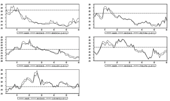
As the results of the out-of-sample forecasts are similar, we constructed

Graph 2 from 60 out-of-sample forecasts for each stock in a time horizon. In

addition, the realized volatility of the last day of the estimation is presented and

kept constant for all forecasts. We observe that theHAR RV andM IDAS

(25)

<GRÁFICO 2 - AQUI>

9 Conclusions

Using the theoretical framework of realized volatility proposed by Andersen

et al. (2003), the goal of this study was to compare two models for volatility

forecasting using the 5 most liquid stocks on the BOVESPA using intraday data

with a 5-minute frequency during a measured period. We used the following

stocks in our study: Bradesco (BBDC4), Petrobrás (PETR4), Vale (VALE5),

Telemar (TNLP4), and Usiminas (USIM5). To correct for the bias of the market

microstructure, we used theM A(q)…lter proposed by Hansen et al. (2008). The

models considered in this study were theHAR RV, proposed by Corsi (2009),

and theM IDAS RV, proposed by Ghysels et al. (2004).

The comparison between the models was performed using in-sample and

out-of-sample measurements of realized volatility. Considering the MSE and

the adjusted R2 _{suggests that the} _{M IDAS} _RV _{model is better than the}

HAR RV model only for in-sample forecasting for the stocks used in our

study. For out-of-sample forecasts, according to the modi…ed Diebold-Mariano

test for the comparison of MSE, there was no signi…cant di¤erence between the

models. Thus, our study suggests that the HAR RV model should be used

for out-of-sample forecasts because of the greater ease of its estimation.

Another important result of this study is the evidence that the use of

(26)

normal distributions, as previously observed for Brazilian data by Carvalho et

al. (2006).

There are numerous possibilities for studies to complement our work here,

mainly related to studies with Brazilian data. For example, we recommend that

future studies consider the e¤ects of the jumps in volatility that we observed in

the data, test other types of …lters for correction of the market microstructure,

and apply other models of realized volatility.

10 Reference

Andersen, T.G. & Bollerslev, T. (1998) Answering the skeptics: Yes,

stan-dard volatility models do provide accurate forecasts. International Economic

Review,39(4), 885–905.

Andersen, T.G.; Bollerslev, T. & Diebold, F.X. (2007) Roughing it up:

In-cluding jump components in the measurement, modeling, and forecasting of

return volatility. The Review of Economics and Statistics,89(4), 701–720.

Andersen, T.G. ; Bollerslev, T. ; Diebold, F.X. & Ebens, H. (2001) The

distribution of realized stock return volatility. Journal of Financial Economics,

61 (1), 43–76.

Andersen, T.G. ; Bollerslev, T.; Diebold, F.X. & Labys, P (2003) Modeling

and forecasting realized volatility. Econometrica,71(2), 579-625.

Barndor¤-Nielsen, O.E. & Shephard, N. (2002) Econometric analysis of

(27)

of the Royal Statistical Society: Series B,64 (2), 253-280.

Carvalho, M.R.C.; Freire, M.A.S.; Medeiros, M.C. & Souza, L.R. (2006)

Modeling and forecasting the volatility of Brazilian asset returns: a realized

variance approach. Revista Brasileira de Finanças,4, 321–343.

Chung, H.M.; Huang, C.S. & Tseng, T.C. (2008) Modeling and

forecast-ing of realized volatility based on high-frequency data: evidence from Taiwan.

International Research Journal of Finance and Economics,22, 178-191.

De Sá Mota, B. & Ferandnes, M. (2004) Desempenho de Estimadores de

Volatilidade na Bolsa de Valores de São Paulo. Revista Brasileira de Finanças,

58, 429-448.

Ebens, H. (1999) Realized stock volatility. mimeo Department of Economics,

Johns Hopkins University.

Forsberg, L. & Ghysels, E. (2006) Why do absolute returns predict volatility

so well? Journal of Financial Econometrics,5(1), 31-67.

Ghysels, E.; Santa-Clara, P.&Valkanov, R. (2004) The Midas touch: mixed

data ampling regression models. minemo CIRANO.

Ghysels, E.; Sinko, A. & alkanov, R. (2007) MIDAS regressions: Further

results and new directions. Econometric Reviews,26, 53-90.

Ghysels, E.; Santa Clara, P. & Valkanov, R (2006) Predicting volatility:

Getting the most out of return data sampled at di¤erent frequencies. Journal

o¤ Econometrics,131, 59-95.

Giot, P. & Laurent, S. (2004) Modelling daily Value-at-Risk using realized

(28)

379-398.

Hansen, P.R.; Large, J. & Lunde, A. (2008) Moving average-based estimators

of integrated variance. Econometric Reviews, 27(1), 79-111.

Harvey, A. C.; Ruiz, E. & Shephard, N. (1994) Multivariate Stochastic

Vari-ance Models. Review of Economic Studies, 61, 247-264.

Harvey, D.; Leybourne, S & Newbold, P. (1997) Testing the equality of

prediction mean squared errors. International Journal of Forecasting, 13 (2),

281-291.

McAleer, M. & Medeiros, M.C. (2008) Realized volatility: a review,

Econo-metric Reviews,27, (1), 10-45.

Oomen, R. (2002) Modelling realized variance when returns are serially

(29)

TABELAS

T a b l e 1 : N u m b e r o f o b s e r v a t i o n s

S t o c k s 5 - m i n p e r i o d 1 5 - m i n p e r i o d 3 0 - m i n p e r i o d B B C D C 4 41:900 15:663 8:330

P E T R 4 45:858 16:142 8:456 VA L E 5 45:532 16:138 8:458 T N L P 4 32:800 14:407 7:947 U S I M 5 40:413 15:475 8:280 S o u r c e : B M & F B O V E S P A

(30)

T a b l e 2 : D e s c r i p t i v e S t a t i s t i c s o f D a i l y R e t u r n s

S t o c k M e a n S . D . A s s K u r t J a r q u e - B e r a B B D C 4 0:00015 0:029 0:678 8:484 0:000 P E T R 4 0:00014 0:031 0:034 6:322 0:000 VA L E 5 0:00023 0:032 0:153 6:284 0:000 T N L P 4 0:00061 0:031 0:470 7:541 0:000 U S I M 5 0:00012 0:035 0:008 6:271 0:000 S o u r c e : O w n c a l c u l a t i o n s

(31)

(32)

T a b l e 4 : D e s c r i p t i v e S t a t i s t i c s o f S t a n d a r d i z e d D a i l y R e t u r n s S t o c k M e a n S . D . A s s K u r t J a r q u e - B e r a

G A R C H

B B D C 4 0;008 1:003 0:216 3:824 0:000 P E T R 4 0:007 0:998 0:140 3:351 0:077 VA L E 5 0:006 1:000 0:224 4:380 0:000 T N L P 4 0:013 1:010 0:412 7:781 0:000 U S I M 5 0:010 1:002 0:078 3:408 0:088

E G A R C H

B B D C 4 0;002 1:000 0:096 3:352 0:130 P E T R 4 0:005 1:000 0:130 3:236 0:207 VA L E 5 0:060 1:000 0:224 4:380 0:000 T N L P 4 0:020 1:019 0:602 1:001 0:000 U S I M 5 0:010 1:003 0:084 4:380 0:093 T a b l e 4 ( c o n t ) : D e s c r i p t i v e S t a t i s t i c s o f S t a n d a r d i z e d D a i l y R e t u r n s

S t o c k M e a n S . D . A s s K u r t J a r q u e - B e r a E W M A

G J R

R E A L I Z E D V O L A T I L I T Y

B B D C 4 0;024 0:949 0:140 2:601 0:049 P E T R 4 0:050 1:047 0:015 2:729 0:388 VA L E 5 0:055 1:040 0:016 2:588 0:114 T N L P 4 0:021 0:964 0:189 2:742 0:070 U S I M 5 0:031 1:028 0:039 2:500 0:038 S o u r c e : O w n c a l c u l a t i o n s

(33)

T a b l e 5 : E s t i m a t e d C o e ¢ c i e n t s o f t h e H A R - RV M o d e l

H o r i z o n t c p - v a l u e d _{p - v a l u e} w _{p - v a l u e} m _{p - v a l u e}

B B D C 4

1 d a y 0:277 0:02 0:165 0:00 0:472 0:00 0:299 0:00 1 w e e k 0:339 0:03 0:171 0:00 0:387 0:00 0:354 0:00 2 w e e k s 0:444 0:01 0:130 0:00 0:401 0:00 0:352 0:00 3 w e e k s 0:529 0:00 0:129 0:00 0:379 0:00 0:353 0:00 4 w e e k s 0:627 0:00 0:119 0:01 0:395 0:01 0:322 0:00

P E T R 4

T a b e l a 5 ( c o n t ) : C o e … c i e n t e s E s t i m a d o s d o M o d e l o H A R - RV

H o r i z o n t e s c p - v a l o r d _{p - v a l o r} w _{p - v a l o r} m _{p - v a l o r}

VA L E 5

1 d i a 0:307 0:02 0:186 0:00 0:476 0:00 0:267 0:00 1 s e m a n a 0:376 0:02 0:151 0:00 0:436 0:00 0:315 0:00 2 s e m a n a s 0:469 0:01 0:130 0:00 0:430 0:00 0:316 0:00 3 s e m a n a s 0:559 0:00 0:127 0:00 0:385 0:00 0:342 0:00 4 s e m a n a s 0:655 0:00 0:114 0:00 0:378 0:00 0:355 0:00

T N L P 4

U S I M 5

1 d a y 0:282 0:04 0:206 0:00 0:303 0:01 0:422 0:00 1 w e e k 0:350 0:05 0:131 0:00 0:323 0:00 0:451 0:00 2 w e e k s 0:459 0:01 0:096 0:00 0:395 0:00 0:383 0:00 3 w e e k s 0:570 0:00 0:098 0:00 0:372 0:00 0:372 0:00 4 w e e k s 0:691 0:00 0:093 0:01 0:375 0:00 0:341 0:00 S o u r c e : O w n c a l c u l a t i o n s

N o t e : C o e ¢ c i e n t s a n d t h e i r r e s p e c t i v e p - v a l u e s r e s u l t i n g f r o m t h e e s t i m a t i o n o f t h e H A R - RV m o d e l s a r e s h o w n , a s d e v e l o p e d b y C o r s i ( 2 0 0 9 ) a n d d e s c r i b e d i n e q u a t i o n ( 1 8 ) , . T h e d a t a w e r e … l t e r e d a c c o r d i n g t o ( 2 8 ) .

(34)

T a b l e 6 : E s t i m a t e d C o e ¢ c i e n t s o f t h e M I D A S - RV M o d e l

B B D C 4

P E T R 4

T a b l e 6 ( c o n t ) : E s t i m a t e d C o e ¢ c i e n t s o f t h e M I D A S - RV M o d e l T h e d a t a w e r e … l t e r e d a c c o r d i n g t o

( 2 6 ) .

VA L E 5

1 d i a 0:307 0:02 0:186 0:00 0:476 0:00 0:267 0:00 1 s e m a n a 0:376 0:02 0:151 0:00 0:436 0:00 0:315 0:00 2 s e m a n a s 0:469 0:01 0:130 0:00 0:430 0:00 0:316 0:00 3 s e m a n a s 0:559 0:00 0:127 0:00 0:385 0:00 0:342 0:00 4 s e m a n a s 0:655 0:00 0:114 0:00 0:378 0:00 0:355 0:00

T N L P 4

U S I M 5

1 d a y 0:282 0:04 0:206 0:00 0:303 0:01 0:422 0:00 1 w e e k 0:350 0:05 0:131 0:00 0:323 0:00 0:451 0:00 2 w e e k s 0:459 0:01 0:096 0:00 0:395 0:00 0:383 0:00 3 w e e k s 0:570 0:00 0:098 0:00 0:372 0:00 0:372 0:00 4 w e e k s 0:691 0:00 0:093 0:01 0:375 0:00 0:341 0:00 S o u r c e : O w n c a l c u l a t i o n s

N o t e : C o e ¢ c i e n t s a n d t h e i r r e s p e c t i v e p - v a l u e s r e s u l t i n g f r o m t h e e s t i m a t i o n o f t h e M I D A S - RV m o d e l s a r e s h o w n , a s d e v e l o p e d b y G h y s e l s e t a l . ( 2 0 0 4 ) , a n d d e s c r i b e d i n e q u a t i o n ( 2 0 ) .

(35)

T a b l e 7 : a d j u s t e dR2

H o r i z o n t B B D C 4 P E T R 4 VA L E 5 T N L P 4 U S I M 5 H A R - RV

1 d a y 0:62 0:60 0:57 0:48 0:56 1 w e e k 0:74 0:75 0:71 0:70 0:71 2 w e e k s 0:73 0:74 0:70 0:71 0:72 3 w e e k s 0:70 0:71 0:67 0:68 0:69 4 w e e k s 0:66 0:68 0:63 0:65 0:65

M I D A S - RV

1 d a y 0:64 0:62 0:58 0:50 0:57 1 w e e k 0:78 0:77 0:75 0:72 0:73 2 w e e k s 0:76 0:76 0:74 0:74 0:75 3 w e e k s 0:74 0:74 0:71 0:73 0:72 4 w e e k s 0:69 0:70 0:67 0:70 0:68 S o u r c e : O w n c a l c u l a t i o n s

N o t e : T h e a d j u s t e dR2_{o f t h e}_HAR _RV_{m o d e l s w e r e} c o n s t r u c t e d t o b e c o m p a r a b l e t o t h o s e o f t h e

(36)

T a b l e 8 : I n - S a m p l e M e a n S q u a r e d E r r o r s ( M S E )

M I D A S - RV

1 d a y 7:26 8:93 10:84 9:83 10:75 1 w e e k 3:35 3:97 4:66 3:60 4:74 2 w e e k s 3:40 3:78 4:48 3:06 4:18 3 w e e k s 3:61 3:99 4:68 3:11 4:38 4 w e e k s 4:11 4:49 5:21 3:33 4:94 F S o u r c e : O w n c a l c u l a t i o n s

(37)

T a b l e 9 : O u t - o f - S a m p l e M e a n S q u a r e d E r r o r s ( M S E )

M I D A S - RV

1 d a y 2:10 2:42 3:23 18:97 3:23 1 w e e k 0:81 1:17 1:35 4:55 1:16 2 w e e k s 1:10 1:15 1:67 3:43 1:04 3 w e e k s 1:47 1:38 1:94 0:93 1:30 4 w e e k s 1:77 1:62 2:16 0:91 1:38 S o u r c e : O w n c a l c u l a t i o n s

(38)

T a b l e 1 0 : O u t - o f - S a m p l e D i e b o l d - M a r i a n o T e s t ( p - v a l u e )

H o r i z o n t B B D C 4 P E T R 4 VA L E 5 T N L P 4 U S I M 5 1 d a y 0:990 0:997 0:999 0:970 0:994 1 w e e k 0:998 0:998 0:994 0:987 0:993 2 w e e k s 0:997 0:997 0:991 0:991 0:993 3 w e e k s 0:993 0:998 0:989 0:994 0:989 4 w e e k s 0:985 0:996 0:983 0:998 0:985 S o u r c e : O w n c a l c u l a t i o n s

(39)

GRAPHS

Figure 1: Daily Realized Volatilities

.00 .02 .04 .06 .08 .10 .12 .14

IV I II III IV I II III IV I II

2008 2009 2010

BBDC4 .00 .04 .08 .12 .16 .20

2008 2009 2010

PETR4 .00 .04 .08 .12 .16 .20

2008 2009 2010

VALE5 .00 .02 .04 .06 .08 .10 .12

2008 2009 2010

TNLP4 .00 .04 .08 .12 .16

2008 2009 2010

USIM5

Source: BM&FBOVESPA

(40)

Figure 2 Out-of-Sample Forecasts .010 .012 .014 .016 .018 .020 .022 .024

10 20 30 40 50 60

HAR M I DA S B B DC4 (t -6 1 )

.010 .012 .014 .016 .018 .020 .022 .024

10 20 30 40 50 60

HAR M I DA S P E T R4 (t -6 1 )

.008 .010 .012 .014 .016 .018 .020 .022 .024 .026

10 20 30 40 50 60

HAR M I DA S V A L E 5 (t -6 1 )

.013 .014 .015 .016 .017 .018 .019 .020 .021

10 20 30 40 50 60

HAR M I DA S T NL P 4 (t -6 1 )

.016 .018 .020 .022 .024 .026 .028

10 20 30 40 50 60