Economic landscapes, what are they? an application to the Brazilian economy and to the sugar cane complex

(1)

Joaquim J.M. Guilhoto1, Marta C. Marjotta-Maistro2, Geoffrey J.D. Hewings3

Abstract

In assessing the economic impact of a sector or group of sectors on a single or multiregional

economy, input-output analysis has proven to be a popular method. . However, there has a problem in

displaying all the information that can be obtained from this analytical approach. In this paper, we have

tried to set new directions in the use of input-output analysis by presenting an improved way of looking

at the economic landscapes. While this is not a new concept, a new meaning is explored in this paper;

essentially, it will now be possible to visualize, in a simple picture, all the relations in the economy as well

as being able to view how one sector is related to the other sectors/regions in the economy. These

relations can be measured in terms of structural changes, production, value added, employment,

imports, etc. While all the possibilities cannot be explored in this paper, the basic idea is given here and

the smart reader can uncover all the various possibilities. To illustrate the power of analysis provided by

the economic landscapes, an application is made to the sugar cane complex using an interregional

input-output system for the Brazilian economy, constructed for 2 regions (Northeast and Rest of Brazil), for

the years of 1985, 1992, and 1995.

1_{University of São Paulo, Brazil and Regional Economics Applications Laboratory (REAL) - University of Illinois,} USA. E-mail: guilhoto@usp.br. This author would like to acknowledge the grant received from the Hewlett Foundation through the Center for Latin American and Caribbean Studies a the University of Illinois.

2_{University of São Paulo, Brazil. E-mail: mcmarjot@carpa.ciagri.usp.br.}

(2)

1. Introduction

In this paper we have worked with a problem faced by many researchers, how to show, in a

compact way, all the vast amount of information contained in input-output tables, and, at the same time,

making it possible to understand what is going on. To do so, this paper takes some new directions

through the use of economic landscapes.

The landscapes concept is not a new one, see for example Sonis, Hewings and Guo (2000), but, it

is given a new meaning in this paper. While all the possibilities are not explored in this paper, the basic

idea is given here and the smart reader can uncover all the various possibilities.

What are they? They are a way of viewing the economy, the axis are the sectors or the agents

involved in the productive process, while the heights are the values resulted from their transaction and

interaction, directly and indirectly. The heights can be values of production, value added, imports,

number of people employed, differences in structural changes, etc.

An application is made considering: a) the Brazilian economy as a whole; and b) the sugar cane

complex in the Northeast and in the Rest of Brazil regions. To undertake the analysis, use is made of an

interregional input-output system for the Brazilian economy, constructed for 2 regions (Northeast and

Rest of Brazil), for the years of 1985, 1992, and 1995.

In the next section, a brief overview of the Brazilian economy is provided as well as the role that

the sugar cane complex has played in the Brazilian economy and in the 2 regions used in the paper. The

third section will make a brief presentation of the methodology. In the fourth section, the landscapes are

presented, while in the last section, some final comments are made.

2. The Brazilian Economy and the Sugar Cane Complex, 1985/1995

This section is divided into three parts; first, a brief overview of the Brazilian economy, then the

general characteristics of the Brazilian macro regions, while the last part will deal with the sugar cane

complex in the Brazilian economy and in the two regions being considered here, the Northeast and the

(3)

2.1. A Brief Overview of the Brazilian Economy in the 1980’s and 1990’s

In the 1980s, the Brazilian economy experienced a very low growth rate especially when

compared to its long run history. In the 1980s, the national GDP grew at a yearly average rate of only

1.56 % (Bonelli and Gonçalves, 1998). The 1990s can be divided into two periods; from 1990 to

1993, the economy went through a period of recession, with the GDP growing at a yearly average rate

of 1.6 %, while industry and agriculture grew at yearly rates of 0.3% and 2.3% respectively. In the

second period, from 1993 to 1997, the yearly average GDP growth rate was of 4.4%, while industry,

agriculture, and services grew, respectively, 3.8%, 6%, and 3.1% (Bonelli and Gonçalves, 1998).

In 1994, investment accounted for 16.3% of Brazilian GDP; in 1995 this share grew to 19.2%

(Baer, 1996 and Conjuntura Econômica, 1997). The quality of the investment also improved and at the

same time there was a growth in the share of imported capital goods. This contributed to an increase in

productivity; with a consequent increase in wages (5.7% in 1993, and 6.2% in 1995) there was also a

decrease in the unemployment rates from 5.3% in 1993 to 4.6% in 1995 (IBGE, 1997a and Conjuntura

Econômica, 1997).

The strong performance of the industrial sector in the 1990 was followed by the growth in

importance of the service sector, mainly due to increased subcontracting by the industrial sector after the

economy was opened up, a process that started in 1990 (Bonelli and Gonçalves, 1998). While the

1980s are characterized by a closed economy, the 1990s can be said to be a decade of openness and

modernization in Brazil.

Finally, we should stress the tendencies and the sectoral progress in the Brazilian economy in the

last decade. The share of the industrial sector in the economy declined from 48% in 1985 to 42% in

1990 and to 34% in 1995, while the service sector’s shares grew respectively from 40%, to 47% and

to 54%. The shares of the agricultural sector were maintained, 12% for 1985, 11% for 1990, and 12%

(4)

2.2. The Brazilian Macro Regions

As show in Figure 1, Brazil is normally divided into five macro regions (IBGE 1997a,b); some

summary characteristics are show in Table 1. Note, in particular, the strong concentration of the national

GDP in the Southeast region, with a share of 56.97%. The Northeast on the other hand, has a much

smaller share in the GDP, 13.62%,

The Northeast region has serious problems of draught and in the beginning of the formation of

the Brazilian State it used to be it most important region, this region has 18.28% of the Brazilian territory

and 28.50% of its population.

(5)

Table 1 - Main Economical and Geographical Characteristics of the Brazilian Macro Regions

Size

Population (1996) Urban Population

GDP 1995 km2 _{Share (%)} Number

(1,000) Share % Share (%)

North 3,851,560 45.25 11,288 7.19 62.36 5.27

Northeast 1,556,001 18.28 44,767 28.50 65.21 13.62

Central West 1,604,852 18.85 10,501 6.69 84.42 7.25

Southeast 924,266 10.85 67,001 42.66 89.29 56.97

South 575,316 6.76 23,514 14.97 77.22 16.89

Brazil 8,511,996 100.00 157,070 100.00 78.36 100.00

Source: IBGE (1997a and 1997b), Considera and Medina (1998).

2.3. The Sugar Cane Complex

During the last decade, the sugar cane complex has gone through a restructuring process

prompted in large part by the government removing its authority to control the trade emanating from the

sugar cane complex, defined as the production of sugar cane, sugar and alcohol in the economy. Until

1990, the sugar cane complex was under the strict control of the federal government, through the Sugar

and Alcohol Institute, which was responsible for the control of production, price, exports, and market

share of the producing Brazilian regions. In 1990, the sugar sector was the first one to be released from

government control, followed by the alcohol sector in 1997. In the new context of a free market

economy, the agents in the process have to learn to survive in a market free from the government rules

and subsidies. Producers have to learn how to be efficient and how to gain market share by attending

the consumer demands, has showed by Marjotta-Maistro (1998).

It is important to put this problem in a historic perspective, given that the Northeast region has

always been a traditional producer of sugar cane, since the colonial period, and it has always been

under the government control. At the same time, the other producing regions are more modern and with

a more market-oriented view. This has had an impact on how the market has reacted to the opening of

(6)

As can be seen in Table 2 and 3, since the 1989/90 the share of the Northeast region in the

sugar cane production has decreased from around 27% to 17%, while the share of land harvested has

decreased from around 34% to 24%, with almost no change in productivity. On the other hand, the

share of the Rest of Brazil has increased as well as it productivity, revealing it to be a more dynamic

region than the Northeast region.

If one looks at the share of the Rest of Brazil region in the production of sugar (Table 4), alcohol

(Table 5), and sugar exports (Table 6), one can see that the share of this region has increase to around

90% in all of the three markets.

Understanding and interpreting these changes will provide the focus of this paper. The next

section will present the theoretical background, with the following section providing the empirical

relation.

Table 2 – Sugar Cane Production (1,000 Ton of Kg) and Share (%) Northeast and Rest of Brazil Regions, 1985/86 to 1998/99

Year Northeast NE Share Rest of Brazil RB Share Total

1985/86 67,645 27.36 179,556 72.64 247,201

1986/87 65,949 27.57 173,230 72.43 239,179

1987/88 80,008 29.80 188,495 70.20 268,503

1988/89 62,851 24.32 195,561 75.68 258,412

1989/90 69,762 27.61 182,881 72.39 252,643

1990/91 71,689 27.29 190,984 72.71 262,673

1991/92 68,730 26.32 192,389 73.68 261,119

1992/93 68,723 25.31 202,752 74.69 271,475

1993/94 39,609 16.20 204,817 83.80 244,426

1994/95 57,328 19.63 234,775 80.37 292,103

1995/96 60,688 19.99 242,869 80.01 303,557

1996/97* 60,652 18.64 264,809 81.36 325,461

1997/98* 65,861 19.52 271,477 80.48 337,338

1998/99* 57,753 17.04 281,219 82.96 338,972

* Includes the production of the North region

(7)

Table 3 –Land of Sugar Cane Harvested (Hectares), Share (%), and Productivity (Ton of Kg per Hectare)

Northeast and Rest of Brazil Regions, 1985/86 to 1998/99 Year Northeast NE Share NE

Productivity

Rest of Brazil

RB

Productivity

RB Share Total

1985/86 1,330,122 34.00 50.86 2,581,943 66.00 69.54 3,912,065 1986/87 1,287,228 32.57 51.23 2,664,614 67.43 65.01 3,951,842 1987/88 1,556,454 36.12 51.40 2,752,221 63.88 68.49 4,308,675 1988/89 1,312,427 31.88 47.89 2,804,948 68.12 69.72 4,117,375 1989/90 1,378,723 33.83 50.60 2,697,116 66.17 67.81 4,075,839 1990/91 1,476,795 34.44 48.54 2,810,830 65.56 67.95 4,287,625 1991/92 1,402,388 33.30 49.01 2,808,503 66.70 68.50 4,210,891 1992/93 1,363,932 32.46 50.39 2,838,572 67.54 71.43 4,202,504 1993/94 1,022,653 27.91 38.73 2,641,069 72.09 77.55 3,663,722 1994/95 1,188,843 27.35 48.22 3,157,141 72.65 74.36 4,345,984 1995/96 1,255,966 27.51 48.32 3,309,695 72.49 73.38 4,565,661 1996/97* 1,229,812 25.43 49.32 3,606,365 74.57 73.43 4,836,177 1997/98* 1,276,329 26.16 51.60 3,603,081 73.84 75.35 4,879,410 1998/99* 1,181,888 23.77 48.87 3,790,125 76.23 74.20 4,972,013

Source: Agrianual (Various Issues)

Table 4 – Sugar Production (1,000 Ton of Kg) and Share (%) Northeast and Rest of Brazil Regions, 1985/86 to 1999/00

Year Northeast* NE Share* Rest of Brazil RB Share Total

1985/86 3,199 40.91 4,620 59.09 7,819

1986/87 3,348 41.04 4,809 58.96 8,157

1987/88 3,158 39.56 4,825 60.44 7,983

1988/89 2,817 34.91 5,253 65.09 8,070

1989/90 3,096 42.79 4,140 57.21 7,236

1990/91 2,857 38.77 4,512 61.23 7,369

1991/92 2,831 32.53 5,873 67.47 8,704

1992/93 3,146 33.40 6,274 66.60 9,420

1993/94 2,318 24.70 7,067 75.30 9,385

1994/95 3,398 28.48 8,535 71.52 11,933

1995/96 3,085 24.88 9,315 75.12 12,400

1996/97 3,950 28.21 10,050 71.79 14,000

1997/98 4,435 27.72 11,565 72.28 16,000

1998/99 3,099 16.93 15,201 83.07 18,300

1999/00 2,115 11.12 16,899 88.88 19,014

(8)

Table 5 – Alcohol Production (Millions of m3) and Share (%) Northeast and Rest of Brazil Regions, 1985/86 to 1999/00

1985/86 2,021 17.10 9,799 82.90 11,820

1986/87 2,215 21.06 8,301 78.94 10,516

1987/88 1,787 15.60 9,667 84.40 11,454

1988/89 1,754 14.97 9,959 85.03 11,713

1989/90 1,980 16.67 9,901 83.33 11,881

1990/91 1,807 15.34 9,976 84.66 11,783

1991/92 1,776 14.01 10,905 85.99 12,681

1992/93 1,672 14.25 10,064 85.75 11,736

1993/94 909 8.06 10,369 91.94 11,278

1994/95 1,579 12.41 11,147 87.59 12,726

1995/96 1,833 14.45 10,856 85.55 12,689

1996/97 1,900 13.54 12,130 86.46 14,030

1997/98 1,700 11.33 13,300 88.67 15,000

1998/99 1,200 8.96 12,200 91.04 13,400

1999/00 1,146 8.97 11,624 91.03 12,770

Source: Associação das Indústrias de Açúcar e Álcool do Estado de São Paulo, USDA, União da Agroindústria Canavieira do Estado de São Paulo.

Table 6 – Sugar Exports (Ton of Kg) and Share (%) Northeast and Rest of Brazil Regions, 1985/86 to 1999/00

1988/89 1,363,921 88.22 182,111 11.78 1,546,032

1989/90 1,250,524 81.39 285,844 18.61 1,536,368

1990/91 1,197,013 85.18 208,269 14.82 1,405,282

1991/92 1,302,528 76.42 401,919 23.58 1,704,447

1992/93 1,312,807 61.21 831,837 38.79 2,144,644

1993/94 862,535 33.76 1,692,454 66.24 2,554,989

1994/95 1,815,924 43.95 2,315,457 56.05 4,131,381

1995/96 1,639,355 36.29 2,877,492 63.71 4,516,847

1996/97 1,484,044 30.90 3,319,430 69.10 4,803,474

1997/98 2,060,711 33.65 4,062,442 66.35 6,123,153

1998/99 819,828 12.76 5,603,272 87.24 6,423,100

* Includes the exports of the North region

(9)

3. Theoretical Background

Define a standard Leontief system:

X = AX+Y (1)

where X is a vector (n x 1) of total production by sector; Y (n x 1) is the final demand; and A is a (n x n) matrix of technical coefficients.

The usual solution is:

X = BY (2)

and

B= −

b

I A

g

−1 (3)

where B (n x n) is the Leontief inverse matrix.

To construct an economic landscape, in production values, to show how the economic system

will work directly and indirectly to produce one unit of the jth sector for the final demand, the A matrix

of direct coefficients is post multiplied by the diagonal of the jth_{column of matrix}

B

d i

B$_•_j , i.e.:

L_j = A B

d i

$_•_j (4)

where Lj is the economic landscape for sector j.

To estimate the economic landscape for a given sector in the economy, in terms of value added,

employment, imports, etc. this can be done by first estimating the coefficient of the value added, for

example, as:

w VA

X k

k

= (5)

where wk is the coefficient of the value added for sector k, VAk is the value added of sector k, and Xk is

the production level of sector k.

After which, it is obtained the value added generated, directly and indirectly, in each sector by

the sale of one unit of sector j to the final demand (vkj), i.e.,

(10)

where bkj is an element of the matrix B defined above.

To obtain the value added matrix of sector j that will be used to construct the value added

economic landscape for this sector (Lw_j ), one first get the share of each direct coefficient in a given row

(eij), then the resulting matrix is post multiplied by the diagonal matrix of vector v. In that way:

e a a ij ij ij i n = =

∑

1 (7)

Lj E V w

j

=

d i

$ ₍₈₎

The next section will present the economic landscapes for the two Brazilian regions considered

in this paper with a particular focus on the sugar cane complex.

4. Economic Landscapes and Structural Changes

In this section, an analysis will be made of the structural changes that took place in the Brazilian

economy from 1985 to 1992 and from 1992 to 1995 at the level of 2 Brazilian regions, Northeast and

Rest of Brazil. After this macro perspective, attention will be directed to how the sugar cane complex

changed in the same time period, for the two regions, and how these changes can the related to the

changes that occurred in the economy as a whole.

4.1. The Brazilian Economy

The information for the analysis of the structural changes in the Brazilian economy are shown in

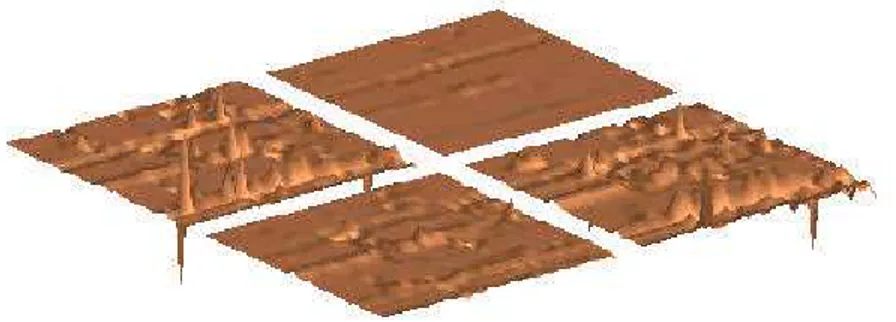
Tables 7 and 8 and displayed in economic landscapes presented in Figures 2 to 5. The economic

landscapes show four blocks: in the upper right corner are the transactions within the Northeast while in

the upper left corner one has the sales from the Northeast region to the Rest of Brazil. In the bottom

part, one has first, the sales from the Rest of Brazil to the Northeast while the final part reveals the

(11)

When comparing the differences among the regions, for 1995, notice that the total height of the

Rest of Brazil region (29.96) is larger than the one for the Northeast region (18.65) implying that the

Rest of Brazil region has a more linked productive process which is an indication of a higher level of

development, confirmed by the data presented into section 2. Concerning the interregional transactions,

one can see that there is a greater dependence of the Northeast region on the Rest of Brazil (total

height value of 6.85) than the Rest of Brazil on the Northeast region (total height value of 1.36).

Table 7 – Sum of the Landscapes Heights from the Leontief Inverse Northeast and Rest of Brazil Regions: 1985, 1992, and 1995

Quadrant 1985 1992 1995

Northeast to Northeast 20.78 20.71 18.65 Northeast to Rest of Brazil 1.64 1.62 1.36 Rest of Brazil to Northeast 10.33 9.97 6.85 Rest of Brazil to Rest of Brazil 34.16 33.92 29.96

Total 66.91 66.22 56.82

Source: Estimated by the authors

Table 8 – Changes and Growth Rates (%) of the Sum of the Landscapes Heights from the Leontief Inverse - Northeast and Rest of Brazil Regions: 1985, 1992, and

1995

Changes Growth Rates (%) Quadrant

1992 – 1985 1995 – 1992 1995 – 1985 1992 – 1985 1995–1992 1995–1985 Northeast to Northeast -0.07 -2.06 -2.12 -0.33 -9.93 -10.23 Northeast to Rest of Brazil -0.02 -0.26 -0.28 -1.26 -16.00 -17.06 Rest of Brazil to Northeast -0.36 -3.12 -3.48 -3.45 -31.33 -33.70 Rest of Brazil to Rest of Brazil -0.24 -3.96 -4.20 -0.71 -11.68 -12.31

Total -0.69 -9.40 -10.09 -1.03 -14.20 -15.08

(12)

The economic landscapes for 1985 and 1995 and the difference between them show that there

was a decrease in the overall height of the economy, given that the amount of production in the

productive process that is necessary to generate of unit of final demand for each one of the 70 sectors

in the economy (35 in each region) has decreased from 66.91 to 56.82. However, this change has not

been equal all over the economy and through time.

From 1985 to 1992, there were practically no changes in the way that the economy behaved as

can be seen in Figure 5 and to the fact that the total value of the heights decreased only from 66.91 to

66.21. The big change occurred from 1992 to 1995 when this value decreased by 14.20% to 56.82.

This can be explained in part by the openness of the economy, started in the 1990’s, that probably has

increased the dependence on imported goods and as a consequence probably decreased the value of

the transactions inside the productive process of the Brazilian economy. This may be and indication of

“hollowing out” (see Hewings et al 1998), whereby an economy becomes more dependent on external

markets for inputs and sales. Clearly, the opening up of the economy contributed to this phenomena.

Also this change was not homogenous through out the two regions in the system, while the

overall decrease of the heights from 1985 to 1995 was of 15.08%, the highest decreases are found in

the transactions among the regions with the heights of the sales from the Northeast to the Rest of Brazil

decreasing by 17.06%, while those from the Rest of Brazil to the Northeast region decreased by

33.70%. Once more this could be the result of the openness process, suggesting that the Northeast

region might have increased its transactions with markets external to the country in place of transactions

with the Rest of Brazil.

Now attention will be directed to the analysis of the sugar cane complex in the Brazilian

(13)

Figure 2 – Economic Landscape of the Leontief Inverse Northeast and Rest of Brazil Regions: 1985

(14)

Figure 4 – Economic Landscape of the Changes in the Leontief Inverse Northeast and Rest of Brazil Regions: 1995 Less 1985

(15)

4.2. The Sugar Cane Complex

Information for the sugar cane complex, consisting of the sugar cane, alcohol, and sugar sectors

is revealed into Tables 9 to 12, in Figures 6 to 11 for the Northeast, and in Tables 13 to 16 and Figures

12 to 17 for the Rest of Brazil. For the Northeast (Tables 9 to 11) it is possible to see that the biggest

changes in the way that the sugar cane complex behaved from 1985 to 1995 occurred in the 1992 to

1995 period, following the overall trend observed for the economy as a whole. The same happened for

the Rest of Brazil (Tables 13 to 16). However, if one looks at Tables 2 to 6 above, it is clear that the

changes occurred in the sugar cane complex of the Northeast were negative, given that the complex has

continuously been loosing market share in the economy, while the sugar cane complex in the Rest of

Brazil region gained market share. This can be explained in part by the fact that the overall heights of the

Sugar Cane complex in the Rest of Brazil are higher than the ones at the Northeast region, meaning a

more modern and integrated complex with the rest of the economy. In addition, the sugar cane complex

in the Northeast decreased its transactions with the Rest of Brazil region, isolating itself from the

modernization process occurred in the Rest of Brazil.

Looking at Figures 6 to 11 for the Northeast, it is clear that the one sector more dependent than

others on inputs from the Rest of Brazil is the sugar sane sector, probably due to the necessity that this

sector has of modern inputs used in the productive process, while the production of alcohol and sugar

depend mainly on the inputs of the sugar cane sector, that are available locally. Also, the overall height

of the alcohol and sugar sectors are larger than the ones of the sugar cane sector meaning that these

sectors have a larger multiplier effect in the economy than the one revealed by the sugar cane sector

alone.

It is also possible to see that the economic landscapes for the relation of inputs inside the

productive process is different from the ones generated when the value added is used. This is clear

when comparing Figures 6, 8, and 10 with, respectively, Figures 7, 9, 11. The share of the value added

generated in each region is given in Table 11, while Table 12 shows the dependence of the total value

added on the transactions that occur in the productive process. Table 12 can be interpreted as a

combination of the information provided in Tables 10 and 11. From Figures 9 and 11, it is clear the

(16)

what was already expected, giving that the sugar cane sector is the main supplier of inputs to both of

these sectors.

Table 9 – Sum of the Landscapes Heights for Inputs and Value Added: Sugar Cane, Alcohol, and Sugar Sectors – Northeast: 1985, 1992, and

1995

Landscape Year Sugar Cane Alcohol Sugar

Inputs 1985 0.33 0.95 1.00

Inputs 1992 0.37 0.95 1.01

Inputs 1995 0.22 0.77 0.87

Value Added 1985 0.97 0.97 0.97

Value Added 1992 0.94 0.95 0.95

Value Added 1995 0.95 0.98 0.98

Table 10 – Share (%) of the Sum of the Landscapes Heights for Inputs in each Quadrant: Sugar Cane, Alcohol, and Sugar Sectors – Northeast: 1985, 1992,

1995

Year Quadrant Sugar Cane Alcohol Sugar

1985 Northeast to Northeast 57.20 86.01 85.74

1985 Northeast to Rest of Brazil 0.70 0.23 0.25 1985 Rest of Brazil to Northeast 22.92 7.18 7.32 1985 Rest of Brazil to Rest of Brazil 19.19 6.58 6.69

(17)

Table 11 – Share (%) of the Value Added in each Region:

Sugar Cane, Alcohol, and Sugar Sectors – Northeast: 1985, 1992, 1995 Year Region Sugar Cane Alcohol Sugar

1985 Northeast 94.49 94.96 94.67

1985 Rest of Brazil 5.51 5.04 5.33

1992 Northeast 92.95 93.45 93.75

1992 Rest of Brazil 7.05 6.55 6.25

1995 Northeast 97.09 98.04 97.70

1995 Rest of Brazil 2.91 1.96 2.30

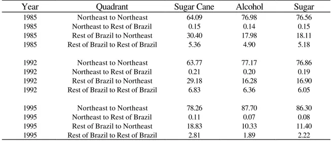
Table 12 – Share (%) of the Sum of the Landscapes Heights for Value Added in each Quadrant: Sugar Cane, Alcohol, and Sugar Sectors

Northeast: 1985, 1992, 1995

(18)

Figure 6 – Economic Landscape for Inputs of the Sugar Cane Sector in the Northeast Region: 1995

(19)

Figure 8 – Economic Landscape for Inputs of the Alcohol Sector in the Northeast Region: 1995

(20)

Figure 10 – Economic Landscape for Inputs of the Sugar Sector in the Northeast Region: 1995

(21)

Table 13 – Sum of the Landscapes Heights for Inputs and Value Added: Sugar Cane, Alcohol, and Sugar Sectors – Rest of Brazil: 1985, 1992, and

1995

Landscape Year Sugar Cane Alcohol Sugar

Inputs 1985 0.46 1.15 1.62

Inputs 1992 0.51 1.11 1.58

Inputs 1995 0.38 0.97 1.50

Value Added 1985 0.93 0.95 0.91

Value Added 1992 0.91 0.92 0.88

Value Added 1995 0.92 0.93 0.87

Table 14 – Share (%) of the Sum of the Landscapes Heights for Inputs in each Quadrant: Sugar Cane, Alcohol, and Sugar Sector

Rest of Brazil: 1985, 1992, 1995

(22)

Table 15 – Share (%) of the Value Added in each Region:

Sugar Cane, Alcohol, and Sugar Sectors – Rest of Brazil: 1985, 1992, 1995 Year Region Sugar Cane Alcohol Sugar

1985 Northeast 1.43 1.34 2.43

1985 Rest of Brazil 98.57 98.66 97.57

1992 Northeast 1.51 1.58 2.32

1992 Rest of Brazil 98.49 98.42 97.68

1995 Northeast 1.28 1.41 3.17

1995 Rest of Brazil 98.72 98.59 96.83

Table 16 – Share (%) of the Sum of the Landscapes Heights for Value Added in each Quadrant: Sugar Cane, Alcohol, and Sugar Sectors

Rest of Brazil: 1985, 1992, 1995

(23)

Figure 12 – Economic Landscape for Inputs of the Sugar Cane Sector in the Rest of Brazil Region: 1995

(24)

Figure 14 – Economic Landscape for Inputs of the Alcohol Sector in the Rest of Brazil Region: 1995

(25)

Figure 16 – Economic Landscape for Inputs of the Sugar Sector in the Rest of Brazil Region: 1995

(26)

For the Rest of Brazil, from Figures 11 to 17, it is possible to see that there are more links

among the sectors than in the Northeast region, which is an indication of more modernity of the sectors,

this is also confirmed by the fact that, as observed above, for the inputs used in the productive process

(Figures 12, 14, and 16) the total sum of the heights are bigger in the Rest of Brazil region (Tables 9 and

13). Considering the dependence of the sectors between the regions (Tables 10, 12, 14, and 16) the

sectors in the Northeast region are more dependent on the sectors of the Rest of Brazil than vice-versa.

As a general conclusion, it is possible to say that the sugar cane complex in the Rest of Brazil

economy has show to be a more modern and dynamic complex when compared to the one in the

Northeast region, and as a result of that has gained share in the market, mainly after 1992 that was

when the openness process started in the economy and the government stepped out from the sector.

5. Final Comments

This paper presented a new concept of analysis through the use of economic landscapes. This

concept can be used to better understand, in a visual way, how the structural changes take place in the

economy as a whole, and how the transactions vary in magnitude and direction among the regions.

Further, The economic landscapes can also be used to determine the relations of a given sector, with the

other sectors and regions.

The use of economic landscapes is illustrated in this paper through an application to the Brazilian

economy and to its Sugar Cane complex, using an interregional input-output system for the Brazilian

economy, constructed for 2 regions (Northeast and Rest of Brazil), for the years of 1985, 1992, and

1995

However, the use of economic landscapes does not replace previous methods of analysis used

with input-output systems; it only uncovers a new and better way of showing information contained in an

input-output table that otherwise would be difficult to analyze and to show to a broader audience of non

(27)

The use of economic landscapes is still in the beginning, and new ways of using it are still to be

discovered. However, a further development is illustrated here, and alternative perspectives will likely

be discovered.

6. References

Agrianual. Various Issues. São Paulo: FNP.

Associação das Indústrias de Açúcar e Álcool do Estado de São Paulo. Boletim Informativo.

Various Issues.

Baer W. (1996). A Economia Brasileira. São Paulo: Nobel.

Bonelli, R., and R.R. Gonçalves (1998). “Para Onde Vai a Estrutura Industrial Brasileira?” In IPEA (1998). A Economia Brasileira em Perspectiva – 1998. Rio de Janeiro: IPEA. Vol. 2, Chapter

16, pp. 617-664.

Conjuntura Econômica (1997). “Indicadores Econômicos,” 51, no. 8.

Considera, C.M. and M.H. Medina (1998). “PIB por Unidade da Federação: Valores Correntes e Constantes – 1985/96”. Rio de Janeiro: IPEA, Texto para Discussão, 610. 32p

Hewings, G.J.D M. Sonis, J. Guo, P. R. Israilevich and G. R. Schindler, (1998) “The hollowing out process in the Chicago economy, 1975-2015,” Geographical Analysis, 30, 217-233

IBGE (1997a). Anuário Estatístico do Brasil 1996, v. 56. Rio de Janeiro.

IBGE (1997b). Contagem da População 1996. Rio de Janeiro.

Marjotta-Maistro, M. C. (1998). Análise do Consumo Industrial de Açúcar no Estado de São Paulo. Master Dissertation. Departamento de Economia, Administração e Sociologia. ESALQ.

University of São Paulo. 100 p. 1998

Melo, H.P., F. Rocha, G Ferraz, G. di Sabbato, R. Dweck (1998) “O Setor Serviços no Brasil: uma Visão Global – 1985/95.” In IPEA (1998). A Economia Brasileira em Perspectiva. Rio de

Janeiro:IPEA. Vol. 2, Chapter 17, pp. 665-712.

Moraes, M.F.D. (2000). A Desregulamentação do Setor Sucroalcooleiro do Brasil.

Sonis, M., G.J.D. Hewings, and J. Guo (2000). “A New Image of Classical Key Sectors Analysis: Minimum Information Decomposition of the Leontief Inverse”. Economic Systems Research. 12

(3). pp. 401-423.

União da Agroindústria Canavieira do Estado de São Paulo. Boletim Informativo. Various Issues.