ALEXANDRE ALONSO ALVES
LINKAGE ANALYSIS AND QRL MAPPING IN SIMULARED POPULARIONS
Rhesis submitted to the Federal University of Viçosa, in partial fulfillment of the requirements of the Genetics and Breeding Graduate Program, for the Degree of Doctor Scientiae.
VIÇOSA
ii
"The only limit to our realization of tomorrow will be our doubts of today. Let us move forward with strong and active faith."
“There are many ways of going forward, but only one way of standing still.”
Franklin D. Roosevelt
To my fiancee, Gisele P. Domiciano
iii
ACKNOWLEDGEMENRS
I am grateful to the Federal University of Viçosa, particularly to the
Genetics and Breeding Graduate Program for the opportunity that was provided
to me in these last years.
I wish to thank the Brazilian National Research Council, CNPq, for the
concession of the PhD scholarship.
I am very grateful to my PhD advisor, Prof Acelino Couto Alfenas, for his
friendship, enthusiasm, patience, and for teaching me the exciting science of
Forest Pathology.
I am also very grateful to Prof Cosme Damião Cruz (PhD co-advisor), for
his unconditional support, for introducing me in the fields of statistical genomics
and biometry, and of course, for helping me in the development of this work.
I wish to especially thank Dr. Lúcio Mauro da Silva Guimarães, Prof.
Leonardo Lopes Bhering and Dr. Marcos Deon Vilela de Resende (PhD co-advisor)
who were always available to discuss ideas and results, and for their friendship.
I am grateful to Dr. Dario Grattapaglia, for his support over the last years
and for introducing me to Eucalyptus genomic research.
I have to express my gratitude to all my professors, in special Prof Sergio
H. Brommonschenkel, for making me see science from a new perspective.
A special thanks to my friends at the Lab of Forest Pathology –
BIOAGRO/UFV for the pleasant times, especially Márcia, Talyta, Marcelo,
Rodrigo, and Ricardo. I also wish to thank my friends at the Labs of Genomics and
iv
I am grateful to my friends in the Graduate programs in Genetics and
Breeding, and Plant Pathology, both from UFV, for providing me an exciting
environment of research, especially Márcio, Ricardo, Leandro and Caio.
Above all, many thanks to my fiancee, Gisele P Domiciano, for being such
a special person in my life and for being always by my side, I love you very much;
to my cockatiels Kiki and Kim (Seseco); to my parents José Donizeti and Vânia
Aparecida; brothers Aléssio and Guilherme; as well as my aunts, Vera, Míriam,
v
RABLE OF CONRENRS
ACKNOWLEDGEMENTS ... iii
TABLE OF CONTENTS ... v
LIST OF TABLES ... vii
LIST OF FIGURES ... ix
RESUMO ... xi
ABSTRACT ... xiv
GENERAL INTRODUCTION ... 1
References ... 8
CHAPTER 1 ... 12
Abstract ... 13
Introduction ... 14
Methods ... 15
Estimation of recombination frequency ... 15
Average Information content and variance of recombination frequency estimators ... 18
Algorithm integration in GQMOL and mapping procedures ... 19
Simulation design and testing ... 19
Results ... 20
Discussion ... 22
Acknowledgements ... 26
References ... 26
Internet Resources ... 27
Supplementary Material ... 34
CHAPTER 2 ... 38
Abstract ... 39
Introduction ... 40
Methods ... 42
Simulations ... 42
Designing of the genomes and parents ... 43
Populations design ... 44
Quantitative traits design ... 44
Linkage and QTL mapping ... 45
vi
Results ... 46
Discussion ... 50
Acknowledgments ... 56
References ... 57
CHAPTER 3 ... 69
Abstract ... 70
Introduction ... 71
Methods ... 73
Simulations ... 73
Genome and parents design ... 73
Full-sib populations design ... 74
Quantitative traits design ... 74
Linkage and QTL mapping ... 75
Comparisons between the pseudo-testcross maps and the full-sib map ... 76
Statistical analysis ... 76
Results ... 77
Linkage mapping analysis ... 77
QTL mapping analysis ... 78
Discussion ... 80
Acknowledgments ... 86
References ... 86
vii
LISR OF RABLES
Chapter 1
Table 1. Likelihood functions and expressions for calculating recombination frequency between dominant and co-dominant markers in full-sib families of out-breeding species (different types of crosses, linkage phases – LP and segregations are considered). ... 28
Table 2. Information content functions relative to all marker configurations involving dominant and co-dominant markers in full-sib families of out-breeding species (different types of crosses, linkage phases – LP, marker configurations -MC and segregations are considered). ... 30
Table 3. Variance of estimated recombination frequencies relative to all marker configurations involving dominant and co-dominant markers in full-sib families of out-breeding species and population size. ... 31
Table S 1. Genotypic frequencies for a progeny derived from a cross between two fully informative co-dominant markers linked in coupling with four alleles *. ... 34
Table S 2. Probability classes and their respective estimates used in likelihood functions*. ... 35
Table S 3. Genotypic frequencies for progenies derived from crosses between different types of co-dominant markers (A locus) and a dominant marker (B locus) for different linkage phases. (In each cross both parents are heterozygous for B locus). ... 36
Chapter 2
viii
Table 2. Summary of QTLs responsible for genetic control of traits designed based on the backcross populations properties………..…………..….60
Table 3. Power of QTL detection with regards to family size and trait heritability by composite interval mapping (CIM) and simple interval mapping (SIM)…..…….61
Table 4. Influence of family size and trait heritability in the precision of QTL mapping by composite interval mapping (CIM)………62
Table 5. Number of times that simple interval mapping (SIM) or composite interval mapping (CIM) detected a ghost QTL instead of the two true QTLs in linkage groups (LG) one and two……….…63
Table 6. Influence of family size and trait heritability in the precision of QTL mapping by simple interval mapping (SIM)……….64
Table 7. Power and precision of QTL mapping by composite interval mapping (CIM) in high density genetic maps compared to mid density maps……….65
Chapter 3
Table 1. Summary of quantitative traits properties in simulated full-sib populations……….89
Table 2. Summary of QTLs responsible for genetic control of traits designed based on the full-sib populations properties……….90
Table 3. Spearman and Pearson correlations, and stress between the pseudo-testcross maps and the full-sib map………..……….….…91
Table 4. Mean size of and mean variance of linkage groups, of both pseudo-testcross maps and of the full-sib map………92
ix
LISR OF FIGURES
Chapter 1
Figure 1. Information content functions relative to all marker configurations involving dominant markers and co-dominant markers in full-sib families of out-breeding species. Configuration 1 refers to crosses A1A1xA1A2; A1A1xA2A3; A1A2xA2A2; A1A2xA3A3 in coupling; configuration 2, to crosses A1A1xA1A2; A1A1xA2A3; A1A2xA2A2; A1A2xA3A3 in repulsion; configuration 3 to cross in A1A2xA1A2 coupling, configuration 4 to cross in A1A2xA1A2 coupling-repulsion; configuration 5 to cross in A1A2xA1A2; configuration 6 to crosses A1A2xA1A3; A1A2xA2A3 and A1A2xA3A4 in coupling; configuration 7 to crosses A1A2xA1A3; A1A2xA2A3 and A1A2xA3A4 in coupling-repulsion; configuration 8 to crosses A1A2xA1A3; A1A2xA2A3 and A1A2xA3A4 in repulsion-coupling and configuration 9 to crosses A1A2xA1A3; A1A2xA2A3 and A1A2xA3A4 in repulsion. ... 32
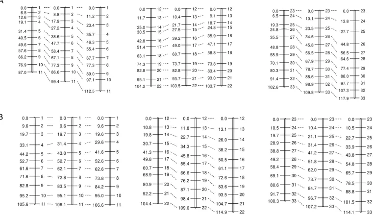
Figure 2. A - simulated genetic map of a full-sib family consisting of three linkage groups and 30 co-dominant markers. B - algorithm-based map of a simulated full-sib family showing the correctly located dominant marker (Marker B – which corresponds to marker 5 in the simulated map). ... 33
Chapter 2
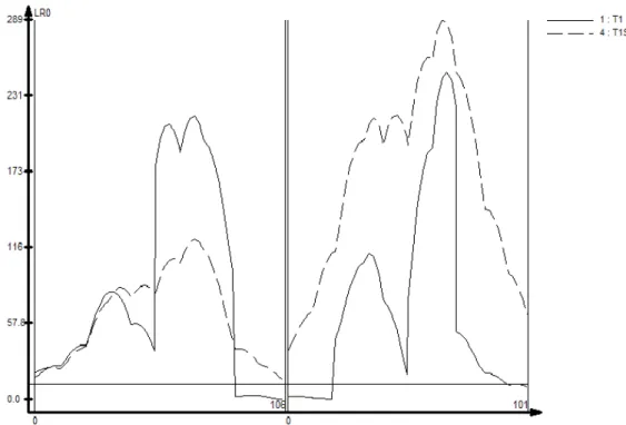
Figure 1. Influence of trait heritability and family size in the accuracy of QTL mapping by composite interval mapping (CIM). A Results here presented refer to the family with n=1000, replicate number 1. Trait 1 (−) (H2=0.8), Trait 2 (- - -) (H2=0.5) and Trait 3 (…..) (H2=0.2). B Results here presented refer to the family with n=100, replicate number 1. Trait 1 (−) (H2=0.8), Trait 2 (- - -) (H2=0.5) and Trait 3 (…..) (H2=0.2). In the X coordinate is shown the linkage groups separated by a double line. Distances are shown in cM. In the Y coordinate is shown the LR scores for each genomic position. A threshold LR score of 12.0 was set (solid horizontal line) to declare significant QTLs………..66
x
double line. Distances are shown in cM. In the Y coordinate is shown the LR scores for each genomic position. A threshold LR score of 12.0 was set (solid horizontal line) to declare significant QTLs. Results here presented refer to the family with n=1000, replicate number 1………67
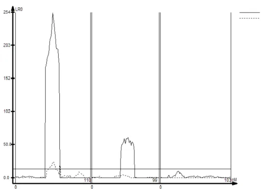
Figure 3. High density maps do not provide a framework to more accurate QTL mapping when compared to mid density maps. Trait 1 (−) (H2=0.8) and Trait 2 (…..) (H2=0.2). In the X coordinate is shown the linkage groups separated by a double line. Distances are shown in cM. In the Y coordinate is shown the LR scores for each genomic position. A threshold LR score of 12.0 was set (solid horizontal line) to declare significant QTLs. Results here presented refer to the family with n=1000, replicate number 1……….…..68
Chapter 3
xi
RESUMO
ALVES, Alexandre Alonso. D.Sc., Universidade Federal de Viçosa, outubro de
2010. Análise de ligação e mapeamento de QRLs em populações simuladas.
Orientador: Acelino Couto Alfenas. Co-orientadores: Cosme Damião Cruz e Marcos Deon Vilela de Resende.
Como os recentes avanços na tecnologia têm levado ao desenvolvimento
de novas tecnologias de genotipagem, no futuro, é mais provável que os mapas
de ligação de alta densidade serão construídos a partir de marcadores
dominantes e co-dominantes. Recentemente, uma abordagem estritamente
genética foi proposta para a estimação da freqüência de recombinação (r) entre
marcadores co-dominantes em famílias de irmãos completos. O conjunto
completo de estimadores quase foi obtido, mas infelizmente, uma configuração
envolvendo a estimativa da distância entre os marcadores dominantes, que
segregam na proporção 3:1 e marcadores co-dominantes, não foi levada em
consideração. Aqui novos nove estimadores são acrescentados ao conjunto
previamente publicado, tornando possível cobrir todas as combinações de
marcadores moleculares com dois a quatro alelos (sem epistasia) em uma família
de irmãos completos. Isso inclui a segregação em um ou ambos os genitores,
dominância e todas as configurações de fases de ligação. Como populações de
retrocruzamentos (RC) são frequentemente utilizadas como populações de
mapeamento, tanto em espécies autógamas, quanto em espécies alógamas foi
conduzido um estudo de simulação para testar as implicações do tamanho da
população, herdabilidade da característica, propriedades do QTL (r2, a e posição)
xii
QTLs. Para tanto foram simuladas populações com diferentes tamanhos, com
diferentes características (h2, número de QTLs e posição) e os dados analisados
com dois métodos de mapeamento de QTLs comumente utilizados
(mapeamento por intervalo simples (MIS) e mapeamento por intervalo
composto (MIC)). Verificou-se que o tamanho da amostra tem uma grande
implicação no poder de detecção e como conseqüência na estimação da
magnitude da variação explicada pelo QTL e no efeito genético, em função de
populações pequenas não permitirem o mapeamento de QTLs de pequeno
efeito, principalmente quando esses estão envolvidos no controle genético de
características de baixa herdabilidade. Também foi verificado que o
posicionamento de QTLs baseados em MIC é mais acurado que MIS e que em
média os QTLs mapeados estavam próximos as suas posições simuladas. Um
resultado interessante é que o MIC tende a subestimar os valores de magnitude
(r2) especialmente em populações grandes/características de baixa herdabilidade
e superestimá-la em populações pequenas, o que pode ser um reflexo do
pequeno coeficiente de variação do erro utilizado, ou devido ao fato de quando
os marcadores não se encontram na exata posição do QTL, esse parâmetro é de
fato esperado ser subestimado. Destaca-se também, o fato que quando
marcadores estão amplamente distribuídos ao longo do genoma (~10cM), e
desse modo cobrindo a região do QTL, se um dos marcadores já estiver próximo
ao QTL, um maior número de marcadores (~1cM) não melhora a precisão do
mapeamento do QTL em populações suficientemente grandes. Baseado nesses
resultados recomenda-se o uso de populações de tamanho adequado, ≥500, se a
intenção é mapear QTLs em populações de RC, porque nessa situação, mesmo
mapas de média densidade podem ser usados para mapear QTLs de grande ou
pequeno efeito com grande confiabilidade. Finalmente, como os procedimentos
de mapeamento de ligação e mapeamento de QTLs em famílias de irmãos
completos (FIC) de espécies alógamas são bastante diversos, foi conduzido um
estudo comparando o método de mapeamento por pseudo-testcross modificado
xiii
em termos de ordenamento dos marcadores, distância entre os marcadores,
comprimento total do mapa, variância das estimativas de distância e estresse.
Investigou-se também o poder de detecção e a precisão de métodos de
mapeamento de QTLs por intervalos baseados nos mapas PST ou no mapa para a
FIC. Verificou-se que em geral as duas estratégias geram mapas altamente
correlacionados com comprimentos dos grupos de ligação proporcionais.
Verificou-se também que independentemente da abordagem de mapeamento
de QTLs utilizadas, o poder de detecção é reduzido em populações pequenas,
especialmente em situações onde a herdabilidade da característica ou
magnitude do QTL é pequena. Também foi verificado que apesar dos dois
métodos serem aparentemente equivalentes em termos de posicionamento do
QTL para características de alta herdabilidade/QTLs de grande efeito, o MIC
baseado nos mapas pseudo-testcross prove dados mais acurados para
características de baixa herdabilidade/QTLs de pequeno efeito. Como relação à
magnitude dos QTLs, notou-se que ambos os métodos parecem ser equivalentes,
sendo os valores superestimados para características de alta herdabilidade e
subestimados para características de baixa herdabilidade, independentemente
do tamanho amostral. Assim para espécies alógamas com médio nível de
recursos genômicos, propõem-se que tanto a abordagem de PST quanto a
abordagem baseada na FIC, e métodos de mapeamento de QTLs relacionados,
possam ser utilizados para gerar mapas genéticos e mapear QTLs com alta
confiabilidade. É importante ressaltar, entretanto, que outros estudos, usando
diferentes cenários, i.e. diferentes coeficientes de variação do erro, diferentes
números de QTLs, diferentes distribuições de marcadores, que coletivamente
podem tornar a simulação um pouco mais realística, são necessários para
xiv
ABSRRACR
ALVES, Alexandre Alonso. D.Sc., Universidade Federal de Viçosa, October, 2010.
Linkage analysis and QRL mapping in simulated populations. Advisor: Acelino
Couto Alfenas. Co-advisors: Cosme Damião Cruz and Marcos Deon Vilela de Resende.
As high-throughput genomic tools have led to the development of novel
genotyping procedures, it is likely that, in the future, high density linkage maps
will be constructed from both dominant and co-dominant markers. Recently, a
strictly genetic approach was described for estimating the recombination
frequency (r) between co-dominant markers in full-sib families. The complete set
of maximum likelihood estimators for r in full-sib families was almost obtained,
but unfortunately, one particular configuration involving dominant markers,
segregating in a 3:1 ratio and co-dominant markers, was not considered. Here we
add nine further estimators to the previously published set, thereby making it
possible to cover all combinations of molecular markers with two to four alleles
(without epistasis) in a full-sib family. This includes segregation in one or both
parents, dominance and all linkage phase configurations. As backcross (BC)
populations are often used as mapping populations both in self pollinating
species, and in out-breeding species we also undertook a simulation study to test
implications of population size, trait heritability, QTL properties (r2, a and
position) and marker density in the power and precision of QTL mapping. For
that we have simulated populations with different sizes, with different
xv
QTL mapping methods (simple interval mapping (SIM) and composite interval
mapping (CIM)). We found that sample size has a major implication in the
detection power and as consequence in the estimation of the magnitude and
additive genetic effect, as small populations do not allow mapping of low effect
QTLs, especially if these QTLs are involved in the genetic control of traits with
low heritability. We also found that the positioning of the QTLs based on CIM is
more accurate than SIM and that on average the mapped QTLs are close to their
simulated position. The results showed that CIM tend to underestimate the
magnitude (r2) values especially in large population sizes/low heritabilities traits
and overestimate it in smaller populations, which can be a reflection of the low
coefficient of variation of the error used, or due to fact that when markers aren´t
in the same of the QTL, this parameter is indeed expected to be underestimated.
We also highlight the fact, that when markers are evenly distributed across the
genome (~10 cM), and therefore covering the QTL region, if one of the markers is
already close to the QTL, larger number of markers (~ 1cM) do not improve the
precision of QTL mapping in sufficiently large mapping populations. Based on our
results we recommend the use of adequate sample size, say ≥500, if the
intention is map QTLs in backcross populations, because in this situation even
mid-density genetic maps can be used to map QTLs of large or small effect with
high confidence. Finally, as the procedures for linkage and QTL mapping in
full-sib families of outbreeding species are quite diverse, we also undertook a
simulation study comparing the modified pseudo-testcross (using SSR markers)
and the full-sib mapping designs in terms of marker ordering, distance between
markers, total map size, distance variance and stress. We also investigated the
power and precision of interval mapping procedures based on the full-sib and on
the modified pseudo-testcross maps. We show that in general the modified
pseudo-testcross and the full-sib mapping designs generate highly correlated
maps with proportional linkage groups length. That independent of the QTL
mapping approach used, detection power is reduced in small populations,
xvi
found that although both methods appear to be equivalent in terms of QTL
positioning for high heritability traits/major effect QTLs, the CIM based on
modified pseudo-testcross maps provide more accurate data for low heritability
traits/minor effect QTLs in larger populations. With regard to QTLs magnitude,
we show that both methods appear to be equivalent, and that the magnitude
values tended to be overestimated for the high heritability trait, and
underestimated for the low heritability trait, independent of the sample size.
Thus, for outbreeding species with mid-level of genomic resources we propose
that either the modified pseudo-testcross or the single full-sib mapping design
and the related QTL mapping strategies can be used to generate genetic maps
and map QTLs with high confidence. It is important to highlight however, that,
other studies, using different scenarios, i.e. different coefficients of variation of
the error, different number of QTLs, different marker distributions, which
collectively may make the simulation a bit more realistic, are needed in order to
1
GENERAL INRRODUCRION
A key development in the field of complex trait analysis was the
establishment of large collections of molecular/genetic markers, which could be
used to construct detailed genetic maps of both experimental and domesticated
species. These maps provided the foundation for the modern-day Quantitative
Trait Loci (QTLs) mapping methodologies (Doerge 2002). A linkage map may be
thought of as a ‘roadmap’ of the chromosomes derived from two different
parents. Linkage maps indicate the position and relative genetic distances
between markers along chromosomes, which is analogous to signs or landmarks
along a highway. The most important use for linkage maps is to identify
chromosomal locations containing genes and QTLs associated with traits of
interest; such maps may then be referred to as genetic maps. Genetic mapping is
based on the principle that genes and, or markers segregate via chromosome
recombination (called crossing-over) during meiosis (i.e. sexual reproduction),
thus allowing their analysis in the progeny (Collard et al. 2005). Genes or markers
that are tightly-linked will be transmitted together from parent to progeny more
frequently than genes or markers that are located further apart (Schuster and
Cruz 2008).
Linkage maps are constructed from the analysis of many segregating
markers. The three main steps of linkage map construction are: (i) production of
a mapping population; (ii) identification of polymorphism and (iii) linkage analysis
of markers. The basis of polymorphism identification, the classes of molecular
2 genotyping can be found elsewhere (Wenzl et al. 2004; Zhu and Salmeron 2007).
The construction of a linkage map requires a segregating plant population (i.e. a
population derived from sexual reproduction). Several different populations may
be utilized for mapping within a given plant species, with each population type
possessing advantages and disadvantages (Collard et al. 2005; Schuster and Cruz
2008). F2 populations, derived from F1 hybrids, and backcross (BC) populations,
derived by crossing the F1 hybrid to one of the parents, are the simplest types of
mapping populations developed for self pollinating species, as well as the most
used. The parents selected to generate the mapping population must differ for
one or more traits of interest, as to allow further QTL/gene mapping. Population
sizes used in preliminary genetic mapping studies generally range from 50 to 250
individuals (Collard et al. 2005), however larger populations are required for
high-resolution mapping. If the map will be used for QTL studies (which is often
the case), then an important point to note is that the mapping population must
be phenotypically evaluated (i.e. trait data must be collected) before subsequent
QTL mapping. The first maximum likelihood estimators of recombination
frequency for a variety of genetic situations in BC and F2 populations were
developed in the early 1950’s (Liu 1997). Linkage theory that subsidizes the
construction of accurate genetic maps has been extensively dealt with in
controlled crosses, and a comprehensive summary of the methods and
techniques can be found in Liu, (1997), Schuster and Cruz (2008) and in excellent
reviews such as Mackay (2001), Doerge (2002) and Collard et al. (2005).
Mapping populations used for mapping cross pollinating species have
been derived from a cross between a heterozygous parent and a haploid or
homozygous parent, or a F1 population, developed by pair crossing heterozygous
parental plants that are distinctly different for important traits (Collard et al.
2005). In cross pollinating species, genetic mapping, however, is more
complicated since most of these species do not tolerate inbreeding. Linkage
analysis in outbreed pedigrees is also complicated by the varying numbers of
3 situation generally gives rise to mixed segregation types (one or both parents
may be heterozygous at each locus), and the linkage phases of markers are
generally unknown. The information content of markers can therefore vary from
one marker locus to the next, depending on the type and dominance of the
marker system used and the type of mapping population (Kirst et al. 2004).
These limitations were partially overcome by new mapping approaches, such as
the pseudo-testcross mapping design (Grattapaglia and Sederoff 1994). This
strategy take advantage of the fact that single-plant genetic linkage maps can be
constructed in outbreed plant species based on single-dose markers that
segregate in testcross configurations in heterozygous individuals (Kirst et al.
2004). In this design each parental derived population is treated as a traditional
backcross (as the genotypes of the individuals can only be 1 or 0) and thus
traditional linkage theory is used either in linkage mapping as in QTL mapping
(discussed on the final part of this section). Linkage analysis of other types of
crosses, i.e. full-sib families and half-sib families derived from highly
heterozygous individuals, was first dealt with by Ott (1985); Ritter et al. (1990);
Arús et al. (1994); Ritter and Salamini (1996); Maliepaard et al. (1997). Together
these papers provided useful formulas for estimating recombination frequency in
almost every situation. Recently, in an extensive work with full-sib families,
Bhering et al. (2008) obtained estimators that differed from those obtained by
Maliepaard et al. (1997), for recombination frequency of different marker
configurations, by using a strictly genetic approach, i.e. the expected proportion
of each phenotypic class in terms of recombination frequency. Based on the
latter, an exogamic population mapping module was implemented in GQMOL
(Cruz 2010) software, extensively used in Brazil for genetic mapping and QTL
analysis.
As previously mentioned, linkage maps provided the foundation for the
modern-day QTL mapping methodologies (Doerge 2002). These techniques
include single-marker mapping, simple interval mapping (SIM) (Lander and
4 Knott (1992) regression or maximum likelihood methods (Zeng 1993, 1994).
These are the main methods used to detect statistical associations between
phenotype and genotype for the purpose of understanding and dissecting the
regions of a genome that affect complex traits in controlled crosses (Doerge
2002; Mackay 2001). In outbreeding species, the associations between
phenotype and genotype have been analyzed in either full-sib or half-sib families
through techniques developed by Fulker and Cardon (1994), Hayashi and Awata
(2004) and, or on random models such as those developed by Goldgar (1990),
Schork (1993) and Xu and Atchley (1995). When the pseudo-testcross design is
used to construct individual genetic maps (Grattapaglia and Sederoff 1994), the
techniques developed for controlled crosses (backcrosses) are often used
(Grattapaglia and Kirst 2008).
Chapter 1
Recent advances in microarray technology and the increasing availability
of genomic information have provided an opportunity to use microarrays to scan
effectively for genetic variations at the whole-genome scale, enabling the
production of high-definition gene-based genetic maps. In a context where,
marker technologies are undergoing a transition from predominantly serial
assays that measure the size of DNA fragments to hybridization-based assays
with high multiplexing levels, three hybridization-based technologies have
emerged: SNP (Single Nucleotide Polymorphisms) (Fan et al. 2006; Ganal et al.
2009; Rafalski 2002), SFP (Single Feature Polymorphism) (Borevitz et al. 2003;
Drost et al. 2009; Zhu and Salmeron 2007) and DArT (Diversity Arrays
Technology) (Jaccoud et al. 2001; Wenzl et al. 2004). As these techniques
generate dominant markers, in the future then, it is most likely that high density
linkage maps will be constructed from both dominant and co-dominant markers
(e.g. SSRs). Such maps will facilitate well-defining the genetic location of
functional markers through flanking high-density co-dominant/dominant
5 dominant marker is often ambiguous, thereby increasing complexity in analysis.
Consequently, the accurate estimation of recombination fractions between
dominant markers and between dominant and co-dominant markers becomes
important.
For F2 with dominant markers, Tan and Fu (2007) recently improved
two-point estimates by taking averages from three-two-point maximum likelihood
estimates, whereas Jansen (2009) developed another method for ordering
dominant markers by minimizing the number of recombinations between
adjacent markers, as a simple alternative to multi-point maximum likelihood.
Recently, in an extensive work with full-sib families, Bhering et al. (2008)
obtained estimators for recombination frequency of different marker
configurations, by using a strictly genetic approach, i.e. the expected proportion
of each phenotypic class in terms of recombination frequency. Unfortunately,
one particular configuration was not dealt with in the mentioned paper, since
distance estimation between dominant markers segregating in a 3:1 ratio and
co-dominant markers, was not taken into consideration. Here, an extension of
Bhering´s work (Bhering et al. 2008) is provided, enabling the estimation of the
recombination frequency between dominant markers segregating in a 3:1 ratio,
and co-dominant markers in full-sib families. The estimators and algorithm were
developed based on the expected frequencies for each genotypic class. These
frequencies were used for building likelihood functions for each possible marker
configuration.
Chapter 2
Quantitative trait loci (QTLs) mapping has been in wide use for nearly two
decades during which molecular markers have become available in conjunction
with interval mapping methods (Borevitz and Chory 2004). Over the past 10
years there has been a tenfold increase in the number of QTL studies published
annually. The goal of QTL mapping is to determine the loci that are responsible
6 is the determination of the number, location and the interaction of these loci
(Borevitz and Chory 2004). Given plentiful markers and high-throughput
genotyping technologies nowadays available (Zhu and Salmeron 2007), QTL
studies have been limited by the need of adequate populations and reliable
phenotypic measures. Experimental design is therefore paramount. As the
accuracy of locating QTL is limited by the number of recombinants that are
identified based on the genotypic states of the markers, sample size and
accurate genotyping becomes important. With this in mind, a commonly asked
question is: Should I genotype more markers on fewer individuals, or score more
individuals (for genotype and phenotype) on fewer markers? Recent methods of
high-throughput genotyping are providing a reliable and cheap mean to
genotype hundreds of individuals with an elevated number of markers, coupled
with high precision. However, because observed recombinants provide the
information, scoring more individuals shall address both previously mentioned
concerns (Doerge 2002). Then one of the most important issues when designing
experimental populations seems to be the sample size.
As backcross (BC) populations are often used as mapping populations
both in self pollinating species (Collard et al. 2005; Doerge 2002), and in
out-breeding species, by means of pseudo-testcross mapping design (Grattapaglia
and Sederoff 1994), a study was undertaken to test the implications of
population size, trait heritability, QTL position and magnitude. For that,
populations of different sizes were simulated, along with three traits with
different heritabilities. Each trait was set to be partially controlled by six QTLs,
each explaining different proportions of the phenotypic variance (from minor to
major effect, linked or unliked). The resulting mapping populations were
analyzed through simple interval mapping (SIM) and composite interval mapping
(CIM) to assess the concern of mapping a ghost QTL in place of the two linked
QTLs.
7 Genetic mapping with outbreeding species, is far more difficult than with
inbreeding species, due to the number of segregating alleles per locus/parent
and the unknown linkage phase of the loci (Bhering et al. 2008). There are a
number of ways to circumvent these complications (Maliepaard et al. 1997). For
highly heterozygous species, such as most of the forest trees (e.g. Eucalyptus
species and hybrids), genetic maps have been developed based mainly on
markers segregating in a double pseudo-testcross configuration in F1 full-sib
families (Grattapaglia and Sederoff 1994). It is now possible however, to
construct a single genetic map for a full-sib family derived of a cross between
two highly heterozygous individuals, based on the information of all markers and
individuals, as it is usually done with populations derived from a cross between
two fully homozygous diploid parents (Alves et al. 2010; Bhering et al. 2008;
Maliepaard et al. 1997). Associations between phenotype and genotype have
been analyzed in full-sib families either based on pseudo-testcross maps or on
single full-sib maps. When the analysis is based on the pseudo-testcross maps, in
most of the cases, interval mapping procedures, such as Composite Interval
Mapping (CIM) (Zeng 1994), are used. When the analysis is based on a full-sib
map, procedures based on Haseman and Elston (1972) regression, such as the
interval mapping technique developed by Fulker and Cardon (1994) are often
used.
As the procedures for linkage and QTL mapping in full-sib families of
outbreeding species are quite diverse, and not readily comparable, we
undertook a simulation study comparing the full-sib and the pseudo-testcross
mapping designs in terms of marker ordering, distance between markers, total
map size, distance variance and stress. We also investigated the power and
precision of interval mapping procedures based on full-sib and on
pseudo-testcross maps. We highlight the implications of population size in linkage and
QTL mapping, along with the implications of trait heritability and QTL properties
8
References
Alves AA, Bhering LL, Cruz CD, Alfenas AC (2010) Linkage analysis between
dominant and co-dominant makers in full-sib families of out-breeding species.
Genetics and Molecular Biology 33:499-506
Arús P, Olarte C, Romero M, Vargas F (1994) Linkage analysis of ten isozyme
genes in F segregating almond progenies. Journal of America Society of
Horticulture Science 119:339-344
Bhering LL, Cruz CD, God PIVG (2008) Estimation of recombination frequency in
genetic mapping of full-sib families. Pesquisa Agropecuária Brasileira
43:363-369
Borevitz JO, Chory J (2004) Genomics tools for QTL analysis and gene discovery.
Curr Opin Plant Biol 7:132-136
Borevitz JO, Liang D, Plouffe D, Chang HS, Zhu T, Weigel D, Berry CC, Winzeler E,
Chory J (2003) Large-scale identification of single-feature polymorphisms in
complex genomes. Genome Research 13:513-523
Collard BCY, Jahufer MZZ, Brouwer JB, Pang ECK (2005) An introduction to
markers, quantitative trait loci (QTL) mapping and marker-assisted selection
for crop improvement: The basic concepts. Euphytica 142:169-196
Cruz CD (2010) GQMOL: a software for quantitative and genetics analysis.
Universidade Federal de Viçosa, Viçosa, MG, Brazil
Doerge RW (2002) Mapping and analysis of quantitative trait loci in experimental
populations. Nat Rev Genet 3:43-52
Drost DR, Novaes E, Boaventura-Novaes C, Benedict CI, Brown RS, Yin TM,
Tuskan GA, Kirst M (2009) A microarray-based genotyping and genetic
mapping approach for highly heterozygous outcrossing species enables
localization of a large fraction of the unassembled Populus trichocarpa
genome sequence. Plant Journal 58:1054-1067
Fan JB, Chee MS, Gunderson KL (2006) Highly parallel genomic assays. Nat Rev
9 Fulker DW, Cardon LR (1994) A sib-pair approach to interval mapping of
quantitative trait loci. American Journal of Human Genetics 54:1092-1103
Ganal MW, Altmann T, Roder MS (2009) SNP identification in crop plants. Curr
Opin Plant Biol 12:211-217
Goldgar DE (1990) Multipoint analysis of human quantitative genetic variation.
American Journal of Human Genetics 47:957-967
Grattapaglia D, Kirst M (2008) Eucalyptus applied genomics: from gene
sequences to breeding tools. New Phytologist 179:911-929
Grattapaglia D, Sederoff R (1994) Genetic-linkage maps of Eucalyptus grandis and
Eucalyptus urophylla using a pseudo-testcross mapping strategy and RAPD
markers. Genetics 137:1121-1137
Haley CS, Knott SA (1992) A simple regressionmethod for mapping quantitative
trait loci in line crosses using flanking markers. Heredity 69:315-324
Haseman JK, Elston RC (1972) Investigation of linkage between a quantitative
trait and a marker locus. Behavior Genetics 2:3-19
Hayashi T, Awata T (2004) Eficient method for analysis of QTL using F1 progenies
in an outcrossing species. Genetica 122:173-183
Jaccoud D, Peng K, Feinstein D, Kilian A (2001) Diversity arrays: a solid state
technology for sequence information independent genotyping. Nucleic Acids
Res 29:E25
Jansen J (2009) Ordering dominant markers in F2 populations. Euphytica
165:401-417
Kirst M, Myburg A, Sederoff R (2004) Genetic mapping in forest trees: markers,
linkage analysis and genomics. In: Setlow JK (ed) Genetic Engineering,
Principles and Methods Kluwer Academic/Plenum Publishers, pp 105-142
Lander ES, Botstein D (1989) Mapping Mendelian factors underlying quantitative
trait using RFLP linkage maps. Genetics 121:185-199
Liu B-H (1997) Statistical genomics: linkage, mapping and QTL analysis. CRC Press,
10 Mackay TFC (2001) The genetic architecture of quantitative traits. Annual Review
of Genetics 35:303-339
Maliepaard C, Jansen J, Van Ooijen JW (1997) Linkage analysis in a full-sib family
of an outbreeding plant species: overview and consequences for applications.
Genetical Research 70:237-250
Ott J (1985) Analysis of human genetic linkage. Johns Hopkins University Press,
Baltimore
Rafalski JA (2002) Novel genetic mapping tools in plants: SNPs and LD-based
approaches. Plant Science 162:329-333
Ritter E, Gebhardt C, Salamini F (1990) Estimation of recombination frequencies
and construction of RFLP linkage maps in plants from crosses between
heterozygous parents. Genetics 125:645-654
Ritter E, Salamini F (1996) The calculation of recombination frequencies in
crosses of allogamous plant species with applications to linkage mapping.
Genetical Research 67:55-65
Schork NJ (1993) Extended multipoint identy-by-descendent analysis of human
quantitative traits: efficiency, power, and modeling considerations. American
Journal of Human Genetics 53:1306-1393
Schuster I, Cruz CD (2008) Estatística Genômica aplicada a populações derivadas
de cruzamentos controlados, 2th edn. Editora UFV, Viçosa
Tan Y-D, Fu Y-X (2007) A new strategy for estimating recombination fractions
between dominant markers from an F2 population. Genetics 175:923-931
Wenzl P, Carling J, Kudrna D, Jaccoud D, Huttner E, Kleinhofs A, Kilian A (2004)
Diversity Arrays Technology (DArT) for whole-genome profiling of barley.
Proceedings of the National Academy of Sciences of the United States of
America 101:9915-9920
Xu S, Atchely WR (1995) A random model approach to interval mapping of
quantitative trait loci. . Genetics 141:1189-1197
Zeng ZB (1993) Theoretical basis of precision mapping of quantitative trait loci.
11 Zeng ZB (1994) Precision mapping of quantitative trait loci. Genetics
136:1457-1468
Zhu T, Salmeron J (2007) High-definition genome profiling for genetic marker
12
CHAPRER 1
LINKAGE ANALYSIS BERWEEN DOMINANR AND CO-DOMINANR MARKERS IN FULL-SIB FAMILIES OF OUR-BREEDING SPECIES
13
Linkage analysis between dominant and co-dominant makers in full-sib families of out-breeding species
Alexandre Alonso Alves1, Leonardo Lopes Bhering2, Cosme Damião Cruz3 and
Acelino Couto Alfenas1
1
Department of Plant Pathology, Federal University of Viçosa, Viçosa, MG, Brazil.
2Embrapa Agroenergy, Parque Estação Biológica, Brasília, DF, Brazil.
3
Department of General Biology, Federal University of Viçosa, Viçosa, MG, Brazil.
Send Correspondence to Acelino Couto Alfenas. Department of Plant Pathology,
Federal University of Viçosa, 36571-000 Viçosa, MG, Brazil. E-mail
Abstract
As high-throughput genomic tools, such as the DNA microarray platform, have
led to the development of novel genotyping procedures, such as Diversity Arrays
Technology (DArT) and Single Nucleotide Polymorphisms (SNPs), it is likely that,
in the future, high density linkage maps will be constructed from both dominant
and co-dominant markers. Recently, a strictly genetic approach was described
for estimating the recombination frequency (r) between co-dominant markers in
full-sib families. The complete set of maximum likelihood estimators for r in
full-sib families was almost obtained, but unfortunately, one particular configuration
involving dominant markers, segregating in a 3:1 ratio and co-dominant markers,
was not considered. Here we add nine further estimators to the previously
published set, thereby making it possible to cover all combinations of molecular
markers with two to four alleles (without epistasis) in a full-sib family. This
includes segregation in one or both parents, dominance and all linkage phase
14
Keywords: statistical genomics, exogamic populations, recombination frequency and maximum likelihood.
Introduction
The first maximum likelihood estimators of recombination frequency for a
variety of genetic situations in BC1 and F2 populations were developed in the
early 1950’s. For F2 with dominant markers, Tan and Fu (2007) recently improved
two-point estimates by taking averages from three-point maximum likelihood
estimates, whereas Jansen (2009) developed another method for ordering
dominant markers by minimizing the number of recombinations between
adjacent markers, as a simple alternative to multi-point maximum likelihood.
Three-point estimates of recombination frequencies were previously used by
Ridout et al. (1998) for out-breeding species. Nevertheless, linkage analysis of
crosses with out-breeders was first dealt with by Ott (1985); Ritter et al. (1990);
Arús et al. (1994); Ritter and Salamini (1996); Maliepaard et al. (1997). Together
these papers provided useful formulas for estimating recombination frequency in
almost every situation. In some cases, the formulas represent the actual
estimators, whereas in others they are likelihood equations requiring
implementation in numerical maximization methods, such as an EM algorithm,
Newton-Raphson, or solved by a graphic method. Recently, in an extensive work
with full-sib families, Bhering et al. (2008) obtained estimators that differed from
those obtained by Maliepaard et al. (1997), for recombination frequency of
different marker configurations, by using a strictly genetic approach, i.e. the
expected proportion of each phenotypic class in terms of recombination
frequency. Based on the latter, an exogamic population mapping module was
implemented in GQMOL (GQMOL, 2009) software, extensively used in Brazil for
genetic mapping and QTL analysis. Unfortunately, one particular configuration
was not dealt with in the mentioned paper, since distance estimation between
dominant markers segregating in a 3:1 ratio and co-dominant markers, was not
15 such as the DNA microarray platform, new dominant genotyping technology has
been developed, such asDArTs (Wenzl et al. 2004) and SNPs. In the future, it is
most likely that high density linkage maps will be constructed from both
dominant and co-dominant markers. Such maps will facilitate well-defining the
genetic location of functional markers through flanking high-density
co-dominant/dominant markers. Nevertheless, due to dominance, the genotype of
an individual at a dominant marker is often ambiguous, thereby increasing
complexity in analysis. Consequently, the accurate estimation of recombination
fractions between dominant markers and between dominant and co-dominant
markers, becomes important (Tan and Fu 2007).
Here, we provide an extension of Bhering´s work, which enables the
estimation of the recombination frequency between dominant markers
segregating in a 3:1 ratio, and co-dominant markers in full-sib families. Our
estimators and algorithm were developed based on the expected frequencies for
each genotypic class. These frequencies were used for building likelihood
functions for each possible marker configuration. Based on intrinsic properties
and their implementation in free linkage software (GQMOL, 2009), this should be
of exceptional use for research groups, whose scope is mapping and the use of
molecular markers for selecting monogenic traits, such as disease resistance,
plant height, and early flowering, amongst other important dominant traits
which are subject to breeding in out-crossing species or constructing high density
genetic maps of both dominant and co-dominant markers.
Methods
Estimation of recombination frequency
In full-sib families, markers may vary in the number of segregating alleles
(up to four), by one or both parents being heterozygous, markers being
dominant or co-dominant, and usually the linkage phases of marker pairs are
unknown. Different types of categories and crossings may occur in the general
16 1972). When considering an A locus with i, j, k and l alleles, there are seven
possible types of crosses (Bhering et al. 2008), but only four are considered to be
informative, since they segregate for at least one parent. Another particularity of
genetic mapping in out-breeding species is that the linkage phase is not known a
priori, as full-sib families are two generation pedigrees. Thus, one has to
considerer four combinations, in order to define the correct linkage phase.
Alleles might be linked by coupling to one of the parents and undefined for the
other, linked by repulsion to one of the parents and undefined for the other,
linked by coupling to both parents, or linked by repulsion to both parents
(Maliepaard et al. 1997). Therefore, the correct linkage phase is usually
determined a posteriori by comparing LOD scores obtained for each combination
(Bhering et al. 2008).
When considering these particularities, the estimation of recombination
frequency (r) in full-sib families may be achieved by using the maximum
likelihood method. With this method, the expected frequencies for each
genotypic class (pi), which are, in turn, dependent on the recombination
frequency between markers (r), are used to built likelihood functions [L(r;ni)],
which, after being maximized for r, give the proper estimator for recombination
frequency. For this, let the genotypes of two individuals of an outbreed
population for a particularly marker, be A1A2 and A3A4, respectively. If these two
individuals are bred to form a full-sib family the expected segregation pattern is:
1A1A3:1A1A4:1A2A3:1A2A4. Now, let the genotypes of these same two individuals
be B1B2 and B3B4 for another marker. If these two individuals are also bred to
form a full-sib family the expected segregation pattern is:
1B1B3:1B1B4:1B2B3:1B2B4.
On considering the haplotypes for the markers in the first parent in the
coupling phase, the produced gametes and their frequencies are: f(A1B1) =
f(A2B2) = (1-r)/2 = P; f(A1B2) = f(A2B1) = r/2 = R, whereas for the second parent,
the expected gametes and frequencies are:f(A3B3) = f(A4B4) = (1-r)/2 = P; f(A3B4) =
17 On now considering gametes produced by these two individuals, 16
genotypic classes are to be expected in the progeny. The genotypic frequencies
for these 16 classes are provided in Table S1. If one now considers that B1 = B3 = B
and B2 = B4 = b, and that BB and Bb are indistinguishable, which typically makes
the B marker dominant, the estimation of recombination frequency between
these two markers can be made by applying the maximum likelihood method.
The likelihood function can be written as:
which is
L(r;ni) = [N!/(nA!....nH!)] x (P2+PR+PR)na x (R2)nb x (P2+PR+R2)nc x (PR)nd x
(P2+PR+R2)ne x (PR)nf x (PR+PR+R2)ng x (P2)nh,
and in its simplified form as:
L(r;ni) = λ(1/4-R2)na(R2)nb(1/4-PR)nc(PR)nd(1/4-PR)ne(PR)nf(1/4-P2)ng(P2)nh
where: PP is (1-r)2/4, PR is r(1-r)/4, RR is r2/4, na is the total number of individuals
with genotypes A1A3B_, nb is the total number of individuals with genotypes
A1A3bb, nc is the total number of individuals with genotypes A1A4B_, nd is the
total number of individuals with genotypes A1A4bb, ne is the total number of
individuals with genotypes A2A3B_, nf is the total number of individuals with
genotypes A2A3rr, ng is the total number of individuals with genotypes A2A4B_, nh
is the total number of individuals with genotypes A2A4bb and N is the total
number of individuals.
The estimate of the recombination fraction is then obtained by the usual
method of maximizing the logarithm of the likelihood function (Table 1).
However, as previously mentioned, different types of crossings may occur
in a full-sib family (Haseman and Elston 1972). Thus, in order to develop general
formulas for estimators of recombination frequency between dominant marker
segregating in a 3:1 ratio and co-dominant makers in full-sib families, one has to
consider all the different segregation patterns and linkage phases for the
co-dominant marker. While the genotypes for the co-dominant will always be Bb (for
both parents), on considering the different types of crosses mentioned above,
18 A1A2xA2A2, A1A2xA1A2; 3 alleles - A1A1xA2A3, A1A2xA3A3, A1A2xA1A3, A1A2xA2A3; 4
alleles - A1A2xA3A4.
So in order to provide an extension of Bhering´s work which would enable
the estimation of recombination frequency between dominant markers
segregating in a 3:1 ratio and co-dominant makers in full-sib families we have
built likelihood functions to estimate the recombination frequency for each
possible marker configuration based on the expected frequencies for each
genotypic class as described above (Tables S2 and S3).
Average Information content and variance of recombination frequency estimators
Bias and variance are important characteristics describing how close one
can get to the true value (Maliepaard et al. 1997). Variances of estimated
recombination fractions can be estimated from average information content (Liu,
1997). Within that context, the general formula for estimating information
content per observation for any single likelihood parameter (θ) is
!"#
" # $
which is -1 times the expectation of the second derivative of the log likelihood
function or the support function with respect to the parameter (θ).
The variance of a maximum likelihood estimate from a sample size of N is
then:
% & '( * )
Since the variances of ML-estimators are approximately equal to the
inverse of Fisher's information, i.e. the expectation of minus the second
derivative of the log-likelihood function (Maliepaard et al. 1997; Schuster and
19
Algorithm integration in GQMOL and mapping procedures
A computer algorithm capable of recognizing the different types of
crosses, segregation and linkage phases, and of calculating recombination
frequency between dominant markers, as well as the co-dominant markers
linked to it based on the likelihood functions here described, was implemented
into GQMOL software (GQMOL, 2009). This first requires the construction of an
integrated linkage map without the dominant marker, according to traditional
methods as described by Ott (1985); Ritter et al. (1990); Arús et al. (1994); Ritter
and Salamini (1996); Maliepaard et al. (1997) and Bhering et al. (2008).
Recombination frequency between the dominant marker and the previously
mapped co-dominant marker, according to the likelihood functions here
described, is then calculated (see results section). In order to define the correct
linkage phase, recombination frequencies are estimated for each of the possible
phases predicted in Table S3, and then compared in terms of LOD scores. By
comparing scores, the algorithm determines the correct linkage phase, and, in
turn, the correct recombination frequency, by identifying the phase and the
associated r that reached the highest LOD score. After determining the
recombination frequency between dominant marker and each of the
co-dominant markers, its position on the previously constructed linkage map is
defined by traditional alignment methods, such as SARF (Sum of Adjacent
Recombination Frequencies) and RCD (Rapid Chain Delineation).
Simulation design and testing
Two hundred (200) individuals segregating for 30 loci were generated
according to Mendelian inheritance at a given recombination frequency. The
simulated genome consisted of 30 markers distributed at an equal distance
throughout three linkage groups. Parents were generated randomly, with four
alleles in equal frequency – 25%, and markers segregated in various
configurations (Haseman and Elston 1972). To build the simulated map,
20 described by Bhering et al. (2008). So as to test the algorithm, data of one
specific marker derived from cross A1A2 x A1A2 was later re-coded as a dominant
marker. Considering that the A1 allele is dominant, data for individuals of
genotypes A1A1 and A1A2 were retyped as 4, and for individuals A2A2 were
retyped as 2 (4 and 2 are the codes used in GQMOL for the genotypes A_ and aa,
respectively). An integrated map without this marker was constructed, as
described by Bhering et al. (2008). Linkage analysis between the dominant and
co-dominant markers was then undertaken, using the functions as presented in
Table 1. Comparisons between the simulated-map and algorithm-map were
carried out in terms of marker ordering, distance between markers, total map
size, distance variance and stress, in order to evaluate whether the algorithm
was efficient as a mapping procedure for dominant markers in full-sib families.
The GQMOL simulation module was used for analysis. Simulation was based on
1000 population replicates.
Results
The genotypic frequencies expected for each marker
configuration/linkage phase combination, including those predicted by Haseman
and Elston (1972), are given in Table S3. Likelihood functions, as well as
estimators of recombination frequency between dominant and co-dominant
markers, for all types of crosses and segregations in full-sib families of
out-breeding species, are given in Table 1. For practical purposes, it is noteworthy
that estimators, which are mainly complex polynomials, have a limited value due
to their high degree. However, with GQMOL, it is possible to circumvent this
limitation by using a graphic method, so that r is calculated directly from
likelihood functions. Hence, different values are attributed to r (in the 0 to 0.5
interval), and LOD score areas calculated for each value. By plotting these scores
on a graph having r values in its x-coordinate, and LOD scores in the
y-coordinate, the highest LOD score is identified on the graph, and the
21 The average information content functions relative to all marker
configurations involving dominant markers and co-dominant markers in full-sib
families of out-breeding species, i.e. different types of crosses, linkage phases,
marker configurations and segregations, is presented in Table 2. These functions
are useful for evaluating the accuracy of recombination frequency by means of
the variance of the estimates. Figure 1 shows that the combinations of dominant
and co-dominant markers in configurations 6, 7, 8 and 9 provided a relatively
large amount of information. These configurations represent crosses between
heterozygous individuals which, according to Haseman and Elston (1972), are the
most informative (Bhering et al. 2008). As to co-dominant markers in
configurations 1, 2, 3, 4 and 5 (some of which are equivalent and have the same
information content function), the functions provided relatively little
information. As in configurations 1 and 2, half the progeny is absolutely
noninformative, the low information content was indeed expected.
Nevertheless, although these latter configurations of dominant and co-dominant
markers appear to provide little information, the variance of its estimators was
quit low. The variances of estimated recombination frequencies (0.05, 0.10 and
0.20), relative to all marker configurations involving dominant markers and
co-dominant markers in full-sib families of out-breeding species and different
population size, are given in Table 3. Here, one can observe that the highest
efficiency is achieved for completely informative co-dominant markers and
crosses (configurations 6, 7, 8 and 9), independent of map saturation, and that
with adequate population sizes (≥ 200 individuals), even non-completely
informative co-dominant markers, together with dominant markers, may be
used for constructing maps. However, if expectation is to obtain a less saturated
map, ideally only co-dominant markers in configurations 6, 7, 8 and 9 should be
selected, in order to correctly map the dominant markers.
The algorithm was tested through simulation. The simulated map is
presented in Figure 2A. Data of one specific locus (marker number 5), derived
22 chi-square (χ2) test, was then re-coded as a dominant marker, as previously
described. As expected, linkage analysis without marker 5 data generated a map
without the marker itself (data not shown). The linkage map generated with our
algorithm and showing marker 5, therein denominated B correctly located in
linkage group 1, is shown in Figure 2B. Comparisons between the simulated-map
and algorithm-map indicated that only linkage group 1 was affected, since
linkage groups 2 and 3 remained exactly the same on both maps. This shows that
the algorithm did not disturb the alignment of the non-involved linkages groups.
Linkage group 1 of the simulated genome was 100.82 cM long, whereas the
algorithm-based map was 100.98 cM. Marker ordering remained unaltered on
the algorithm map, with a mean marker distance of 12.63 cM, while on the
simulated map, the mean distance between markers was 12.60 cM. Map
variance increased from 15.97 on the simulated map to 17.66 on the
algorithm-based. Spearman correlation, which measures map ordering consistence, was
near 1, thereby indicating that the algorithm, and, in turn, the functions and
estimators, were efficient in locating dominant markers. On the other hand,
Pearson correlation, which measures correlations between marker distances,
was 0.93, thereby also indicating the efficiency of both algorithm and formulas.
However, as can be seen in Figures 2A and 2B, the distances between the so
called B marker and the 4 and 6 markers are slightly different from those
estimated between marker 5 and 4 and 6 on the simulated map.
Discussion
Since most of the computer packages used for genetic mapping are not
capable of analyzing out-breeding populations, with the exception of JoinMap
(Stam, 1993), over the past years, we have been developing a free genetic
software named GQMOL (GQMOL, 2009), apt at analyzing, through genetic
mapping, QTL mapping and simulation, not only controlled crosses, but also
full-sib and half-full-sib families. So as to implement an out-breeding population mapping
23 estimators for different marker configurations. However, GQMOL was still inept
at estimating the distance between dominant and co-dominant markers. Here,
we provide an extension of Bhering´s work, apt at estimating recombination
frequency between a dominant marker segregating in a 3:1 ratio and
co-dominant markers in full-sib families. Likelihood functions, used for estimating
recombination frequency between the dominant marker and co-dominant
markers for each possible marker configuration predicted by Haseman and
Elston (1972), were built based on the expected frequencies for each genotype
class in a strictly genetic approach. By maximizing the natural logarithm of the
log-likelihood functions, the estimators for the recombination frequency
between the two markers were obtained. It is noteworthy that our estimators
(including those presented in Bhering et al. 2008) are quite different from those
obtained by Maliepaard et al. (1997). These differences are due to the fact that
we have applied a strictly genetic approach, rather than a genetic-statistical
approach (iterative procedure - EM algorithm) as used by Maliepaard et al.
(1997). Both methods appear to be equivalent, since the same data packages
analyzed by JoinMap and GQMOL resulted in nearly alike integrated maps (AA
Alves – unpublished data). However, in situations where the likelihood function
is very flat (i.e., the data provide little information due to dominance and
markers being in the repulsion phase), the estimates obtained by the EM
algorithm may depend on the starting value for recombination frequency. An
overall view of likelihood through graphic procedures, or the explicit likelihood
function solution, could possibly give rise to recombination frequency associated
with the true maximum in a more reliable way. Our method, apart from being
simple, may then be more applicable to a wider range of situations than the
methods currently available.
A simple simulation approach was chosen to test our algorithm. A
simulated full-sib family was generated for the purpose, and data from one
specific marker re-coded for dominance, followed by linkage analyses with our