Linkage analysis between dominant and co-dominant makers in full-sib families of out-breeding species

Linkage analysis between dominant and co-dominant makers in full-sib

families of out-breeding species

Alexandre Alonso Alves

, Leonardo Lopes Bhering

, Cosme Damião Cruz

and Acelino Couto Alfenas

Departamento de Fitopatologia, Universidade Federal de Viçosa, Viçosa, MG, Brazil.

2

_{Embrapa Agroenergia, Parque Estação Biológica, Brasília, DF, Brazil.}

3

_{Departamento de Biologia Geral, Universidade Federal de Viçosa, Viçosa, MG, Brazil.}

Abstract

As high-throughput genomic tools, such as the DNA microarray platform, have lead to the development of novel genotyping procedures, such as Diversity Arrays Technology (DArT) and Single Nucleotide Polymorphisms (SNPs), it is likely that, in the future, high density linkage maps will be constructed from both dominant and co-dominant mark-ers. Recently, a strictly genetic approach was described for estimating recombination frequency (r) between co-dominant markers in full-sib families. The complete set of maximum likelihood estimators forr in full-sib families was almost obtained, but unfortunately, one particular configuration involving dominant markers, segregating in a 3:1 ratio and co-dominant markers, was not considered. Here we add nine further estimators to the previously published set, thereby making it possible to cover all combinations of molecular markers with two to four alleles (without epistasis) in a full-sib family. This includes segregation in one or both parents, dominance and all linkage phase con-figurations.

Key words:statistical genomics, exogamic populations, recombination frequency and maximum likelihood.

Received: June 23, 2009; Accepted: January 26, 2010.

Introduction

The first maximum likelihood estimators of recombi-nation frequency for a variety of genetic situations in BC1

and F2populations were developed in the early 1950’s. For

F2with dominant markers, Tan and Fu (2007) recently

im-proved two-point estimates by taking averages from three-point maximum likelihood estimates, whereas Jansen (2009) developed another method for ordering dominant markers by minimizing the number of recombinations be-tween adjacent markers, as a simple alternative to multi-point maximum likelihood. Three-multi-point estimates of re-combination frequencies were previously used by Ridoutet al.(1998) for out-breeding species. Nevertheless, linkage analysis of crosses with out-breeders was first dealt with by Ott (1985); Ritteret al.(1990); Arúset al.(1994); Ritter and Salamini (1996); Maliepaardet al. (1997). Together these papers provided useful formulas for estimating re-combination frequency in almost every situation. In some cases, the formulas represent actual estimators, whereas in others they are likelihood equations requiring implementa-tion in numerical maximizaimplementa-tion methods, such as an EM al-gorithm, Newton-Raphson, or solved by a graphic method. Recently, in an extensive work with full-sib families,

Bheringet al.(2008) obtained estimators that differed from those obtained by Maliepaardet al.(1997), for recombina-tion frequency of different marker configurarecombina-tions, by using a strictly genetic approach,i.e.the expected proportion of each phenotypic class in terms of recombination frequency. Based on the latter, an exogamic population mapping mod-ule was implemented in GQMOL (GQMOL, 2009) soft-ware, extensively used in Brazil for genetic mapping and QTL analysis. Unfortunately, one particular configuration was not dealt with in the mentioned paper, since distance estimation between dominant markers segregating in a 3:1 ratio and co-dominant markers, was not taken into consid-eration. With the advent of high-throughput genomic tools, such as the DNA microarray platform, new dominant geno-typing technology has been developed, such as DArTs (Wenzl et al., 2004) and SNPs. In the future, it is most likely that high density linkage maps will be constructed from both dominant and co-dominant markers. Such maps will facilitate well-defining the genetic location of func-tional markers through flanking high-density co-domi-nant/dominant markers. Nevertheless, due to dominance, the genotype of an individual at a dominant marker is often ambiguous, thereby increasing complexity in analysis. Consequently, the accurate estimation of recombination fractions between dominant markers and between domi-Send Correspondence to Acelino Couto Alfenas. Departamento de

Fitopatologia, Universidade Federal de Viçosa, 36571-000 Viçosa, MG, Brazil. E-mail [email protected].

nant and co-dominant markers, becomes important (Tan and Fu, 2007).

Here, we provide an extension of Bherings work, which enables the estimation of the recombination fre-quency between dominant markers segregating in a 3:1 ratio, and co-dominant markers in full-sib families. Our es-timators and algorithm were developed based on the ex-pected frequencies for each genotypic class. These frequen-cies were used for building likelihood functions for each possible marker configuration. Based on intrinsic proper-ties and their implementation in free linkage software (GQMOL, 2009), this should be of exceptional use for re-search groups, whose scope is mapping and the use of mo-lecular markers for selecting monogenic traits, such as dis-ease resistance, plant height, and early flowering, amongst other important dominant traits which are subject to breed-ing in out-crossbreed-ing species or constructbreed-ing high density ge-netic maps of both dominant and co-dominant markers.

Methods

Estimation of recombination frequency

In full-sib families, markers may vary in the number of segregating alleles (up to four), by one or both parents being heterozygous, markers being dominant or co-do-minant, and usually the linkage phases of marker pairs are unknown. Different types of categories and crossings may occur in the general case of multi-allelic systems with four or more alleles (Haseman and Elston, 1972). When consid-ering an A locus with i, j, k and l alleles, there are seven pos-sible types of crosses (Bheringet al., 2008), but only four are considered to be informative, since they segregate for at least one parent. Another particularity of genetic mapping in out-breeding species is that the linkage phase is not knowna priori, as full-sib families are two generation pedi-grees. Thus, one has to considerer four combinations, in or-der to define the correct linkage phase. Alleles might be linked by coupling to one of the parents and undefined for the other, linked by repulsion to one of the parents and un-defined for the other, linked by coupling to both parents, or linked by repulsion to both parents (Maliepaard et al., 1997). Therefore, the correct linkage phase is usually deter-mineda posterioriby comparing LOD scores obtained for each combination (Bheringet al., 2008).

When considering these particularities, the estima-tion of recombinaestima-tion frequency (r) in full-sib families may be achieved by using the maximum likelihood method. With this method, the expected frequencies for each geno-typic class (pi), which are, in turn, dependent on the recom-bination frequency between markers (r), are used to built likelihood functions [L(r;ni)], which, after being maxi-mized forr, give the proper estimator for recombination frequency. For this, let the genotypes of two individuals of an outbreed population for a particularly marker, be A1A2

and A3A4, respectively. If these two individuals are bred to

form a full-sib family the expected segregation pattern is: 1A1A3:1A1A4:1A2A3:1A2A4. Now, let the genotypes of

these same two individuals be B1B2and B3B4for another

marker. If these two individuals are also bred to form a full-sib family the expected segregation pattern is: 1B1B3:1B1B4:1B2B3:1B2B4.

On considering the haplotypes for the markers in the first parent in the coupling phase, the produced gametes and their frequencies are: f(A1B1) = f(A2B2) = (1-r)/2 = P;

f(A1B2) = f(A2B1) = r/2 = R, whereas for the second parent,

the expected gametes and frequencies are: f(A3B3) =

f(A4B4) = (1-r)/2 = P; f(A3B4) = f(A4B3) = r/2 = R.

On now considering gametes produced by these two individuals, 16 genotypic classes are to be expected in the progeny. The genotypic frequencies for these 16 classes are provided in Table S1. If one now considers that B1= B3= B

and B2= B4= b, and that BB and Bb are indistinguishable,

which typically makes the B marker dominant, the estima-tion of recombinaestima-tion frequency between these two mark-ers can be made by applying the maximum likelihood method. The likelihood function can be written as:

L(r, n )_i p_in i a

h

i =

=

Õ

which is

L(r;ni) = [N!/(nA!....nH!)] x (P2+PR+PR)nax (R2)nbx

(P2+PR+R2)ncx (PR)ndx (P2+PR+R2)nex (PR)nfx (PR+PR+R2)ngx (P2)nh,

and in its simplified form as:

L(r;ni) =l(1/4-R2)na(R2)nb(1/4-PR)nc(PR)nd (1/4-PR)ne(PR)nf(1/4-P2)ng(P2)nh

where PP is (1-r)2/4, PR is r(1-r)/4, RR is r2/4, nais the total

number of individuals with genotypes A1A3B_, nbis the

to-tal number of individuals with genotypes A1A3bb, ncis the

total number of individuals with genotypes A1A4B_, ndis

the total number of individuals with genotypes A1A4bb, ne

is the total number of individuals with genotypes A2A3B_,

nfis the total number of individuals with genotypes A2A3rr,

ng is the total number of individuals with genotypes

A2A4B_, nhis the total number of individuals with

geno-types A2A4bb and N is the total number of individuals.

The estimate of the recombination fraction is then ob-tained by the usual method of maximizing the logarithm of the likelihood function (Table 1).

dif-ferent types of crosses mentioned above, the genotypes for the co-dominant marker may be: 2 alleles - A1A1xA1A2,

A1A2xA2A2, A1A2xA1A2; 3 alleles - A1A1xA2A3,

A1A2xA3A3, A1A2xA1A3, A1A2xA2A3; 4 alleles

-A1A2xA3A4.

So in order to provide an extension of Bherings work which would enable the estimation of recombination fre-quency between dominant markers segregating in a 3:1 ra-tio and co-dominant makers in full-sib families we have built likelihood functions to estimate the recombination frequency for each possible marker configuration based on the expected frequencies for each genotypic class as de-scribed above (Tables S2 and S3).

Average Information content and variance of recombination frequency estimators

Bias and variance are important characteristics de-scribing how close one can get to the true value (Malie-paardet al., 1997). Variances of estimated recombination fractions can be estimated from average information con-tent (Liu, 1997). Within that context, the general formula for estimating information content per observation for any single likelihood parameter (q) is

I( )q E ¶ log ( | )L x E log ( |L

¶q q ¶ ¶q q q q = é ëê ù ûú é ë ê ê ù û ú ú=

-2 2 2 x) é ë ê ù û ú

which is -1 times the expectation of the second derivative of the log likelihood function or the support function with re-spect to the parameter (q).

The variance of a maximum likelihood estimate from a sample size of N is then:

s q q 2 1 ($) ( ) = N I

Since the variances of ML-estimators are approxi-mately equal to the inverse of Fisher’s information,i.e.the expectation of minus the second derivative of the log-likelihood function (Maliepaardet al., 1997 and Schuster and Cruz, 2004), we used this approach to obtain the re-spective functions.

Algorithm integration in GQMOL and mapping procedures

A computer algorithm capable of recognizing the dif-ferent types of crosses, segregation and linkage phases, and of calculating recombination frequency between dominant markers, as well as the co-dominant markers linked to it based on the likelihood functions here described, was im-plemented into GQMOL software (GQMOL, 2009). This first requires the construction of an integrated linkage map without the dominant marker, according to traditional methods as described by Ott (1985); Ritteret al.(1990);

Arúset al.(1994); Ritter and Salamini (1996); Maliepaard

et al.(1997) and Bheringet al.(2008). Recombination

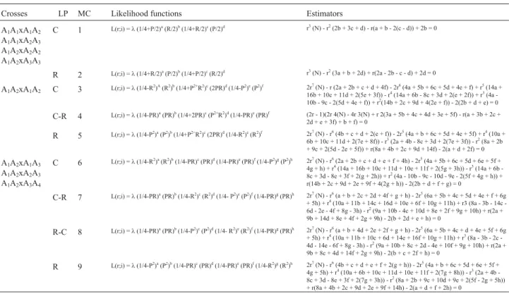
fre-Table 1- Likelihood functions and expressions for calculating recombination frequency between dominant and co-dominant markers in full-sib families of out-breeding species (different types of crosses, linkage phases - LP and segregations are considered).

Crosses LP MC Likelihood functions Estimators

A1A1xA1A2 A1A1xA2A3 A1A2xA2A2 A1A2xA3A3

C 1 L(r;i) =l(1/4+P/2)a

(R/2)b

(1/4+R/2)c

(P/2)d _r3

(N) - r2

(2b + 3c + d) - r(a + b - 2(c - d)) + 2b = 0

R 2 L(r;i) =l(1/4+R/2)a

(P/2)b

(1/4+P/2)c

(R/2)d _r3

(N) - r2

(3a + b + 2d) + r(2a - 2b - c - d) + 2d = 0

A1A2xA1A2 C 3 L(r;i) =l(1/4-R

2 )A (R2 )b (1/4+P2+ R2 )c (2PR)d (1/4-P2 )e (P2

)f _2r7

(N) - r (2a + 2b + c + d + 4f) - 2r6

(4a + 5b + 6c + 5d + 4e + f) + r5

(14a + 16b + 10c + 11d + 2(5e + 3f)) - r4

(14a + 6b - 8c + 3d + 2(e + 2f)) + r3

(4a -10b - 9c - 2(5d + 4e + f)) + r2

(14b + 2c + 9d + 4(2e + f)) - 2(2b + d + e) = 0

C-R 4 L(r;i) =l(1/4-PR)a

(PR)b (1/4+2PR)c (P2+ R2 )d (1/4-PR)e

(PR)f _{(2r - 1)(2r 4(N) - 4r 3(N) + r 2(3a + 5b + 4c + 4d + 3e + 5f) - r(a + 3b + 2c +}

2d + e + 3f) + b + f) = 0

R 5 L(r;i) =l(1/4-P2

)a (P2 )b (1/4+P2+ R2 )c (2PR)d (1/4-R2 )e (R2

)f _2r7

(N) - r6

(4b + c + d + 2(e + f)) - 2r5

(4a + b + 6c + 5d + 4e + 5f) + r4

(10a + 6b + 10c + 11d + 2(7e + 8f)) - r3

(2a + 4b - 8c + 3d + 2(7e + 3f)) - r2

(8a + 2b + 9c + 2(5d - 2e + 5f)) + r(8a + 4b + 2c + 9d + 14f) - 2(a + d + 2f) = 0

A1A2xA1A3 A1A2xA2A3 A1A2xA3A4

C 6 L(r;i) =l(1/4-R2

)a (R2 )b (1/4-PR)c (PR)d (1/4-PR)e (PR)f (1/4-P2 )g (P2

)h _2r7

(N) - r6

(2a + 2b + c + d + e + f + 4h) - 2r5

(4a + 5b + 6c + 5d + 6e + 5f + 4g + h) + r4_{(14a + 16b + 10c + 11d + 10e + 11f + 2(5g + 3h)) - r}3_{(14a + 6b}

-8c + 3d - 8e + 3f + 2(g + 2h)) + r2

(4a - 10b - 9c - 10d - 9e - 2(5f + 4g + h)) + r(14b + 2c + 9d + 2e + 9f + 4(2g + h)) - 2(2b + d + f + g) = 0

C-R 7 L(r;i) =l(1/4-PR)a

(PR)b

(1/4-R2

)c

(R2

)d

(1/4- P2

)e

(P2

)f

(1/4-PR)g

(PR)h _2r7

(N) - r6

(a + b + 2c + 2d + 4f + g + h) - 2r5

(6a + 5b + 4c + 5d + 4e + f + 6g + 5h) + r4

(10a + 11b + 14c + 16d + 10e + 6f + 10g + 11h) + r3 (8a 3b 14c -6d - 2e - 4f + 8g - 3h) - r2_{(9a + 10b - 4c + 10d + 8e + 2f + 9g + 10h) + r(2a +}

9b + 14d + 8e + 4f + 2g + 9h) - 2(b + 2d + e + h) = 0

R-C 8 L(r;i) =l(1/4-PR)a

(PR)b

(1/4-P2

)c

(P2

)d

(1/4- R2

)e

(R2

)f

(1/4-PR)g

(PR)h _2r7

(N) - r6

(a + b + 4d + 2e + 2f + g + h) - 2r5

(6a + 5b + 4c + d + 4e + 5f + 6g + 5h) + r4

(10a + 11b + 10c + 6d + 14e + 16f + 10g + 11h) + r3

(8a 3b 2c -4d - 14e - 6f + 8g - 3h) - r2

(9a + 10b + 8c + 2d - 4e + 10f + 9g + 10h) + r(2a + 9b + 8c + 4d + 14f + 2g + 9h) - 2(b + c + 2f + h) = 0

R 9 L(r;i) =l(1/4-P2

)a (P2 )b (1/4-PR)c (PR)d (1/4-PR)e (PR)f (1/4-R2 )g (R2

)h _2r7

(N) - r6

(4b + c + d + e + f + 2(g + h)) - 2r5

(4a + b + 6c + 5d + 6e + 5f + 4g + 5h) + r4

(10a + 6b + 10c + 11d + 10e + 11f + 2(7g + 8h)) - r3

(2a + 4b -8c + 3d - 8e + 3f + 2(7g + 3h)) - r2

quency between the dominant marker and the previously mapped co-dominant marker, according to the likelihood functions here described, is then calculated (see results sec-tion). In order to define the correct linkage phase, recombi-nation frequencies are estimated for each of the possible phases predicted in Table S3, and then compared in terms of LOD scores. By comparing scores, the algorithm deter-mines the correct linkage phase, and, in turn, the correct re-combination frequency, by identifying the phase and the associatedrthat reached the highest LOD score. After de-termining the recombination frequency between dominant marker and each of the co-dominant markers, its position on the previously constructed linkage map is defined by tra-ditional alignment methods, such as SARF (Sum of Adja-cent Recombination Frequencies) and RCD (Rapid Chain Delineation).

Simulation design and testing

Two hundred (200) individuals segregating for 30 loci were generated according to Mendelian inheritance at a given recombination frequency. The simulated genome consisted of 30 markers distributed at an equal distance throughout three linkage groups. Parents were generated randomly, with four alleles in equal frequency - 25%, and markers segregated in various configurations (Haseman and Elston, 1972). To build the simulated map, recombina-tion frequency and LOD scores were calculated using for-mulas as described by Bheringet al.(2008). So as to test the algorithm, data of one specific marker derived from cross A1A2 x A1A2 was later re-coded as a dominant marker.

Considering that the A1 allele is dominant, data for individ-uals of genotypes A1A1and A1A2were retyped as 4, and for

individuals A2A2were retyped as 2 (4 and 2 are the codes

used in GQMOL for the genotypes A_ and aa, respec-tively). An integrated map without this marker was con-structed, as described by Bhering et al. (2008). Linkage analysis between the dominant and co-dominant markers was then undertaken, using the functions as presented in Table 1. Comparisons between thesimulated-mapand

al-gorithm-mapwere carried out in terms of marker ordering,

distance between markers, total map size, distance variance and stress, in order to evaluate whether the algorithm was efficient as a mapping procedure for dominant markers in full-sib families. A GQMOL simulation module was used for analysis. Simulation was based on 1000 population rep-licates.

Results

The genotypic frequencies expected for each marker configuration/linkage phase combination, including those predicted by Haseman and Elston (1972), are given in Ta-ble S3. Likelihood functions, as well as estimators of re-combination frequency between dominant and co-domi-nant markers, for all types of crosses and segregations in full-sib families of out-breeding species, are given in

Ta-ble 1. For practical purposes, it is noteworthy that estimators, which are mainly complex polynomials, have a limited value due to their high degree. However, with GQMOL, it is possible to circumvent this limitation by us-ing a graphic method, so thatris calculated directly from likelihood functions. Hence, different values are attributed tor(in the 0 to 0.5 interval), and LOD score areas calcu-lated for each value. By plotting these scores on a graph havingrvalues in its x-coordinate, and LOD scores in the y-coordinate, the highest LOD score is identified on the graph, and the corresponding r value on the abscissa (Schuster and Cruz, 2004).

The average information content functions relative to all marker configurations involving dominant markers and co-dominant markers in full-sib families of out-breeding species, i.e. different types of crosses, linkage phases, marker configurations and segregations, are presented in Table 2. These functions are useful for evaluating the accu-racy of recombination frequency by means of the variance of the estimates. Figure 1 shows that the combinations of dominant and co-dominant markers in configurations6,7,

8and9provided a relatively large amount of information. These configurations represent crosses between heterozy-gous individuals which, according to Haseman and Elston (1972), are the most informative (Bheringet al.2008). As to co-dominant markers in configurations1,2,3,4 and5

(some of which are equivalent and have the same informa-tion content funcinforma-tion), the funcinforma-tions provided relatively lit-tle information. As in configurations 1 and 2, half the progeny is absolutely noninformative, the low information content was indeed expected. Nevertheless, although these latter configurations of dominant and co-dominant markers appear to provide little information, the variance of its esti-mators was quit low. The variances of estimated recombi-nation frequencies (0.05, 0.10 and 0.20), relative to all marker configurations involving dominant markers and co-dominant markers in full-sib families of out-breeding species and different population size, are given in Table 3. Here, one can observe that the highest efficiency is achieved for completely informative co-dominant markers and crosses (configurations6,7,8and9), independent of map saturation, and that with adequate population sizes (³200 individuals), even non-completely informative co-dominant markers, together with co-dominant markers, may be used for constructing maps. However, if expectation is to obtain a less saturated map, ideally only co-dominant markers in configurations6,7,8and9should be selected, in order to correctly map dominant markers.

The algorithm was tested through simulation. The

simulated mapis presented in Figure 2A. Data of one

spe-cific locus (marker number 5), derived from cross type A1A2xA1A2, and that segregated in a 1:2:1 ratio as

marker itself (data not shown). The linkage map generated with our algorithm and showing marker 5, therein denomi-nated B and correctly located in linkage group 1, is shown in Figure 2B. Comparisons between thesimulated-mapand

algorithm-mapindicated that only linkage group 1 was

af-fected, since linkage groups 2 and 3 remained exactly the same on both maps. This shows that the algorithm did not disturb the alignment of the non-involved linkages groups.

Linkage group 1 of thesimulated genomewas 100.82 cM long, whereas the algorithm-based map was 100.98 cM. Marker ordering remained unaltered on thealgorithm map, with a mean marker distance of 12.63 cM, while on the

sim-ulated map, the mean distance between markers was

12.60 cM. Map variance increased from 15.97 on the

simu-lated mapto 17.66 on thealgorithm-based. Spearman

cor-relation, which measures map ordering consistence, was near 1, thereby indicating that the algorithm, and, in turn, the functions and estimators, were efficient in locating dominant markers. On the other hand, Pearson correlation, which measures correlations between marker distances, was 0.93, thereby also indicating the efficiency of both al-gorithm and formulas. However, as can be seen in Figures 2A and 2B, the distances between the so called B marker and the 4 and 6 markers are slightly different from those es-timated between marker 5 and 4 and 6 on thesimulated

map.

Discussion

Since most of the computer packages used for genetic mapping are not capable of analyzing out-breeding popula-tions, with the exception of JoinMap (Stam, 1993), over the past years, we have been developing a free genetic software named GQMOL (GQMOL, 2009), apt at analyzing, through genetic mapping, QTL mapping and simulation, not only controlled crosses, but also full-sib and half-sib families. So as to implement an out-breeding population mapping module in GQMOL, Bheringet al.(2008) devel-oped likelihood functions and estimators for different marker configurations. However, GQMOL was still inept at estimating the distance between dominant and co-do-minant markers. Here, we provide an extension of Bherings work, apt at estimating recombination frequency between a dominant marker segregating in a 3:1 ratio and

co-do-Table 2- Information content functions relative to all marker configurations involving dominant and co-dominant markers in full-sib families of out-breeding species (different types of crosses, linkage phases - LP, marker configurations -MC and segregations are considered).

Crosses LP MC Function

A1A1xA1A2 A1A1xA2A3 A1A2xA2A2 A1A2xA3A3

C 1 - [12r2- 12r - 2] / [r(r + 1)(r - 1)(r - 2)]

R 2 -[12r2_{- 12r - 2] / [r(r + 1)(r - 1)(r - 2)]}

A1A2xA1A2 C 3 -[84r6- 60r5- 250r4+ 268r3- 63r2- 70r + 37] / [r(r + 1) (r - 1) (r - 2) (r2- r + 1) (r2+ 2r - 1)] C-R 4 -[120r4_{- 240r}3_{+ 216r}2_{- 96r + 16] / [r(r - 1) (r}2_{- r + 1) (2r}2_{- 2r + 1)]}

R 5 -[84r6- 60r5- 250r4+ 268r3- 63r2- 70r + 37] / [r(r + 1) (r - 1) (r - 2) (r2- r + 1) (r2+ 2r - 1)] A1A2xA1A3

A1A2xA2A3 A1A2xA3A4

C 6 -[4(28r6- 18^5- 90r4+ 88r3- 12r2- 27r + 12)] / [r(r + 1) (r - 1) (r - 2) (r2- r + 1 )(r2+ 2r - 1)]

C-R 7 -[112r6_{- 72r}5_{- 360r}4_{+ 352r}3_{- 48r}2_{- 108r + 48] / [r(r + 1) (r - 1) (r - 2) (r}2_{- r + 1) (r}2_{+ 2r - 1)]} R-C 8 -[112r6- 72r5- 360r4+ 352r3- 48r2- 108r + 48] / [r(r + 1) (r - 1) (r - 2) (r2- r + 1) (r2+ 2r - 1)] R 9 -[4(28r6- 18r5- 90r4+ 88r3- 12r2- 27r + 12)] / [r(r + 1) (r - 1) (r - 2) (r2- r + 1) (r2+ 2r - 1)]

Figure 2- A - simulated genetic map of a full-sib family consisting of three linkage groups and 30 co-dominant markers. B - algorithm-based map of a simulated full-sib family showing the correctly located dominant marker (Marker B - which corresponds to marker 5 in the simulated map).

Table 3- Variance of estimated recombination frequencies relative to all marker configurations involving dominant and co-dominant markers in full-sib families of out-breeding species and population size.

Marker configuration Population size (n)

r = 0.05 100 200 400 800 1000

1and2** 3.78429* 1.892145 0.946072 0.473036 0.378428988

3and5 0.249117 0.124558 0.062279 0.03114 0.024911692

4 0.349641 0.174821 0.08741 0.043705 0.034964109

6,7,8and9 0.195527 0.097763 0.048882 0.024441 0.019552669

r = 0.1 100 200 400 800 1000

1and2 6.107143 3.053571 1.526786 0.763393 0.610714286

3and5 0.456649 0.228324 0.114162 0.057081 0.045664893

4 0.806025 0.403012 0.201506 0.100753 0.080602496

6,7,8and9 0.365124 0.182562 0.091281 0.04564 0.036512396

r = 0.2 100 200 400 800 1000

1and2 8.816327 4.408163 2.204082 1.102041 0.881632653

3and5 0.731963 0.365981 0.182991 0.091495 0.073196286

4 2.462069 1.231034 0.615517 0.307759 0.246206897

6,7,8and9 0.608783 0.304392 0.152196 0.076098 0.060878318

*Values were multiplied by 104_.

minant markers in full-sib families. Likelihood functions, used for estimating recombination frequency between the dominant marker and co-dominant markers for each possi-ble marker configuration predicted by Haseman and Elston (1972), were built based on the expected frequencies for each genotype class in a strictly genetic approach. By maxi-mizing the natural logarithm of the log-likelihood func-tions, the estimators for the recombination frequency between the two markers were obtained. It is noteworthy that our estimators (including those presented in Bheringet al.2008) are quite different from those obtained by Malie-paardet al.(1997). These differences are due to the fact that we have applied a strictly genetic approach, rather than a genetic-statistical approach (iterative procedure - EM algo-rithm) as used by Maliepaardet al.(1997). Both methods appear to be equivalent, since the same data packages ana-lyzed by JoinMap and GQMOL resulted in nearly alike in-tegrated maps (AA Alves - unpublished data). However, in situations where the likelihood function is very flat (i.e., the data provide little information due to dominance and mark-ers being in the repulsion phase), the estimates obtained by the EM algorithm may depend on the starting value for re-combination frequency. An overall view of likelihood through graphic procedures, or the explicit likelihood func-tion solufunc-tion, could possibly give rise to recombinafunc-tion fre-quency associated with the true maximum in a more reliable way. Our method, apart from being simple, may then be more applicable to a wider range of situations than the methods currently available.

A simple simulation approach was chosen to test our algorithm. A simulated full-sib family was generated for the purpose, and data from one specific marker re-coded for dominance, followed by linkage analyses with our algo-rithm. The dominant marker was correctly located in the linkage map generated with the algorithm, and Spearman and Pearson correlations indicated its efficiency in locating the dominant marker without disturbing nearby markers or other linkage groups. Nevertheless, we noticed that the dis-tances between the dominant marker and those flanking were slightly different from those previously obtained be-tween marker 5 and markers 4 and 6. This was probably due to the loss of information with re-coded data. Whereas three genotypic classes (2 heterozygotes and one homozygote) can be analyzed with co-dominant markers, with dominant markers one can analyze only two (dominant and reces-sive). This may have affected estimates of recombination frequencies, thereby resulting in different map distances. However, for practical purposes,e.g., MAS - marker as-sisted selection, bias in distance is not expected to be a problem. Traditional mapping strategies based on co-domi-nant markers also locate markers near their real position, with an expected bias (Schuster and Cruz, 2004). Our algo-rithm then, proved to be very fast and precise, and its only prior requirement is a linkage map without the dominant

marker constructed following traditional methods as de-scribed by Bheringet al.(2008) or Maliepaardet al.(1997). As to the accuracy of estimates, it has long been rec-ognized that dominant markers in the repulsion linkage phase supply low linkage information content in F2

popula-tions. Nowadays, this problem is receiving additional atten-tion, as high-throughput genomic tools, such as the DNA microarray platform, have lead to the development of up-to-date genotyping procedures resulting in new dominant markers. Novel methods for mapping such markers circum-venting this issue have been described (Tan and Fu, 2007; Jansen, 2009). Nevertheless, in full-sib families of out-breeding species, dominant markers appear to be unim-peachable, if used together with co-dominant markers. Our variances estimates for three distinct values of recombina-tion frequency (0.05, 0.10 and 0.20), all marker configura-tions involving dominant markers and co-dominant markers in full-sib families of out-breeding species and dif-ferent population size indicates that variances of recombi-nation frequency estimates are very low, ranging from 0.060878318 x 10-4for completely informative markers in a large population (n = 1000) to 8.816327 x 10-4for par-tially informative markers in a small population (n = 100). These values are very similar to the estimates obtained from co-dominant markers in F2populations, and

consider-able lower when compared to estimates from both co-dominant and co-dominant markers in F2. For example, for

re-combination frequencies of 0.05, 0.10 and 0.20, variance estimates for co-dominant markers in an F2of 200

individu-als were 1.25 x 10-4, 2.53 x 10-4and 5.23 x 10-4, respectively (Schuster and Cruz, 2004; Liu, 1997). The variance esti-mates for co-dominant and dominant markers in the very same F2were 2.47 x 10-4, 4.91 x 10-4and 9.69 x 10-4,

respec-tively, (Schuster and Cruz, 2004; Liu, 1997). As recombi-nation frequency estimator variance is comprised of two main components, viz., the number of recombination events that created the progeny sample and the (in) ability with which these events can be detected for a certain con-figuration of two loci, it is reasonable to speculate that the first is defined by recombination frequency itself and prog-eny size, and the second by the segregation types of loci and linkage phases in the parents (Maliepaard et al., 1997). Hence, although the particularities of out-breeding species (number of segregating alleles and different linkage phases) represent an enormous challenge for genetic map-ping, these may, on the other hand, contribute to more accu-rate estimates of recombination frequency.

summary, by this paper and Bheringet al.(2008), an over-view of the whole range of situations of molecular markers in crosses with out-breeding species (full-sib families), has been presented from a genetic perspective. Based on its properties and implementation into free linkage software, our approach should be useful for those interested in using molecular markers for mapping, or as an aid in selecting out-crossing species.

Acknowledgments

We are grateful to Phil Cannon, for his constructive comments on the manuscript. The Bioinformatics Lab of the Federal University of Viçosa, Brazil provided the facili-ties for the development of this work. This work was also supported by the Brazilian National Research Council, CNPq, with a Ph.D. fellowship to AAA and a research fel-lowship to ACA and CDC.

References

Arús P, Olarte C, Romero M and Vargas F (1994) Linkage analy-sis of ten isozyme genes in F segregating almond progenies. J Am Soc Hortic Sci 119:339-344.

Bhering LL, Cruz CD and God PIVG (2008) Estimation of recom-bination frequency in genetic mapping of full-sib families. Pesq Agropec Bras 43:363-369.

Haseman JK and Elston RC (1972) The investigation of linkage between a quantitative trait and a marker locus. Behav Genet 2:3-19.

Jansen J (2009) Ordering dominant markers in F2 populations. Euphytica 165:401-417.

Liu B-H (1997) Statistical genomics: Linkage, mapping and QTL analysis. CRC Press, Boca Raton, 648 pp.

Maliepaard C, Jansen J and Van Ooijen JW (1997) Linkage analy-sis in a full-sib family of an outbreeding plant species: Over-view and consequences for applications. Genet Res 70:237-250.

Ott J (1985) Analysis of Human Genetic Linkage. Johns Hopkins University Press, Baltimore, 223 pp.

Ridout MS, Tong S, Vowden CJ and Tobutt KR (1998) Three-point linkage analysis in crosses of allogamous plant spe-cies. Genet Res 72:111-121.

Ritter E and Salamini F (1996) The calculation of recombination frequencies in crosses of allogamous plant species with ap-plications to linkage mapping. Genet Res 67:55-65. Ritter E, Gebhardt C and Salamini F (1990) Estimation of

recom-bination frequencies and construction of RFLP linkage maps in plants from crosses between heterozygous parents. Genet-ics 125:645-654.

Schuster I and Cruz CD (2004) Estatística Genômica Aplicada a Populações Derivadas de Cruzamentos Controlados. UFV Press, Viçosa, 568 pp.

Stam P (1993) Construction of integrated genetic linkage maps by means of a new computer package: JoinMap. Plant J 3:739-744.

Tan Y-D and Fu Y-X (2007) A new strategy for estimating recom-bination fractions between dominant markers from an F2 population. Genetics 175:923-931.

Wenzl P, Carling J, Kudrna D, Jaccoud D, Huttner E, Kleinhofs A and Kilian A (2004) Diversity Arrays Technology (DArT) for whole-genome profiling of barley. Proc Natl Acad Sci USA 101:9915-9920.

Internet Resources

GQMOL (2009) Quantitative and Molecular Genetics Software, http://www.ufv.br/dbg/gqmol/gqmol.htm (October 9, 2009).

Supplementary Material

The following online material is available for this article: Table S1 Genotypic frequencies for a progeny derived from a

cross between two fully informative co-dominant markers linked in coupling with four alleles.

Table S2 Probability classes and their respective estimates used in likelihood functions

Table S3 Genotypic frequencies for progenies derived from crosses between different types of co-dominant markers and a dominant marker for different linkage phases.

This material is made available as part of the online article from http://www.scielo.br.gmb.

Associate Editor: Paulo A. Otto

Individuals Class Genotypic frequency

A1A3B1B3 PP (1 - r)2/4

A1A3B1B4 PR r(1 - r)/4

A1A4B1B3 PR r(1 - r)/4

A1A4B1B4 PP (1 - r)2/4

A1A3B2B3 PR r(1 - r)/4

A1A3B2B4 RR r2/4

A1A4B2B3 RR r2/4

A1A4B2B4 PR r(1 - r)/4

A2A3B1B3 PR r(1 - r)/4

A2A3B1B4 RR r2/4

A2A4B1B3 RR r2/4

A2A4B1B4 PR r(1 - r)/4

A2A3B2B3 PP (1 - r)

2 /4

A2A3B2B4 PR r(1 - r)/4

A2A4B2B3 PR r(1 - r)/4

A2A4B2B4 PP (1 - r)2/4

*P = (1 - r)/2; R = r/2; P + R = 0.5.

Probabilities Estimates

P2 (1 - r)2/4

R2 _r2_/4

P/2 (1 - r)/4

R/2 r/4

PR (r - r2_)/4

2PR (r - r2)/2

1/4 - P2 _{(2r - r}2_)/4

1/4 - R2 (1 - r2)/4

1/4 - PR (r2- r + 1)/4

1/4 + P/2 (2 - r)/4

1/4 + R/2 (r + 1)/4

1/4 + 2PR (2r2_{- 2r - 1)/4}

PR + PR + P2 _{(1 - r}2_)/4

PR + PR + R2 (2r - r2)/4

1/4 + P2_{+ R}2 _(r2_{- r + 1)/4}

P2+ R2 (2r2- 2r + 1)/4

Cross Segregation Coupling Cou-Rep Rep-Cou Repulsion

A1A1xA1A2 A1A1B_ 1/4 + P/2 - - 1/4 + R/2

A1A1bb R/2 - - P/2

A1A2B_ 1/4 + R/2 - - 1/4 + P/2

A1A2bb P/2 - - R/2

A1A1xA2A3 A1A2B_ 1/4 + P/2 - - 1/4 + R/2

A1A2bb R/2 - - P/2

A1A3B_ 1/4 + R/2 - - 1/4 + P/2

A1A3bb P/2 - - R/2

A1A2xA2A2 A1A2B_ 1/4 + P/2 - - 1/4 + R/2

A1A2bb R/2 - - P/2

A2A2B_ 1/4 + R/2 - - 1/4 + P/2

A2A2bb P/2 - - R/2

A1A2xA3A3 A1A3B_ 1/4 + P/2 - - 1/4 + R/2

A1A3bb R/2 - - P/2

A2A3B_ 1/4 + R/2 - - 1/4 + P/2

A2A3bb P/2 - - R/2

A1A2xA1A2 A1A1B_ 1/4 - R2 1/4 - PR - 1/4 - P2

A1A1bb R2 PR - P2

A1A2B_ 1/4 + P2+ R2 1/4 + 2PR - 1/4 + P2+ R2

A1A2bb 2PR P2+ R2 - 2PR

A2A2B_ 1/4 - P2 1/4 - PR - 1/4 - R2

A2A2bb P2 PR - R2

A1A2xA1A3 A1A1B_ 1/4 - R2 1/4 - PR 1/4 - PR 1/4 - P2

A1A1bb R2 PR PR P2

A1A3B_ 1/4 - PR 1/4 - R2 1/4 - P2 1/4 - PR

A1A3bb PR R2 P2 PR

A1A2B_ 1/4 - PR 1/4 - P2 1/4 - R2 1/4 - PR

A1A2bb PR P2 R2 PR

A2A3B_ 1/4 - P2 1/4 - PR 1/4 - PR 1/4 - R2

A2A3bb P2 PR PR R2

A1A2xA2A3 A1A2B_ 1/4 - R2 1/4 - PR 1/4 - PR 1/4 - P2

A1A2bb R2 PR PR P2

A1A3B_ 1/4 - PR 1/4 - R2 1/4 - P2 1/4 - PR

A1A3bb PR R2 P2 PR

A2A2B_ 1/4 - PR 1/4 - P2 1/4 - R2 1/4 - PR

A2A2bb PR P2 R2 PR

A2A3B_ 1/4 - P2 1/4 - PR 1/4 - PR 1/4 - R2

A2A3bb P2 PR PR R2

A1A2xA3A4 A1A3B_ 1/4 - R2 1/4 - PR 1/4 - PR 1/4 - P2

A1A3bb R2 PR PR P2

A1A4B_ 1/4 - PR 1/4 - R2 1/4 - P2 1/4 - PR

A1A4bb PR R2 P2 PR

A2A3B_ 1/4 - PR 1/4 - P2 1/4 - R2 1/4 - PR

A2A3bb PR P2 R2 PR

A2A4B_ 1/4 - P2 1/4 - PR 1/4 - PR 1/4 - R2