The potential for material processing in hydrological systems – a novel classification approach

(1)

HESSD

9, 10487–10524, 2012

The potential for material processing

in hydrological systems

C. E. Oldham et al.

Title Page

Abstract Introduction

Conclusions References

Tables Figures

◭ ◮

Back Close

Full Screen / Esc

Printer-friendly Version Interactive Discussion

Discussion

P

a

per

|

Dis

cussion

P

a

per

|

Discussion

P

a

per

|

Discussio

n

P

a

per

|

Hydrol. Earth Syst. Sci. Discuss., 9, 10487–10524, 2012 www.hydrol-earth-syst-sci-discuss.net/9/10487/2012/ doi:10.5194/hessd-9-10487-2012

Hydrology and Earth System Sciences Discussions

This discussion paper is/has been under review for the journal Hydrology and Earth System Sciences (HESS). Please refer to the corresponding final paper in HESS if available.

The potential for material processing

in hydrological systems – a novel

classification approach

C. E. Oldham1, D. E. Farrow2, and S. Peiffer3

1

School of Environmental Systems Engineering, The University of Western Australia, 35 Stirling Hwy, Crawley Western Australia 6009, Australia

2

Mathematics and Statistics, Murdoch University, Murdoch Western Australia 6150, Australia 3

Department of Hydrology, University of Bayreuth, Germany

Received: 15 August 2012 – Accepted: 5 September 2012 – Published: 18 September 2012

Correspondence to: C. E. Oldham (carolyn.oldham@uwa.edu.au)

(2)

HESSD

9, 10487–10524, 2012

C. E. Oldham et al.

Title Page

Tables Figures

◭ ◮

Back Close

Full Screen / Esc

Discussion

P

a

per

|

Dis

cussion

P

a

per

|

Discussion

P

a

per

|

Discussio

n

P

a

per

|

Abstract

Assessing the potential for transfer or export of biogeochemicals or pollutants from catchments is of primary importance under changing land use and climatic condi-tions. Over the past decade the connectivity/disconnectivity dynamic of a catchment has been related to its potential to export material, however we continue to use multiple

5

definitions of connectivity, and most have focused strongly on physical (hydrologicaly or hydraulic) connectivity. In this paper we use a dual-lens approach, where the dynamic balance between transport and reaction is constantly in focus, and define ecohydrolog-ical connectivity as the ability of matter and organisms to transfer within and between elements of the hydrologic cycle while undergoing biogeochemical transformation. The

10

connectivity/disconnectivity dynamic must take into account the opportunity for a given reaction to occur during transport and/or isolation. Using this definition, we define three distinct regimes: (1) one which is ecohydrologically connected and diffusion dominated; (2) one which is ecohydrologically connected and advection dominated and (3) one which is both hydrologically and ecohydrologically disconnected. Within each regime

15

we use a new non-dimensional number,NE, to compare exposure timescales with

re-actions timescales.NEis reaction-specific and allows the estimation of relevant spatial

scales over which the reactions of interest are taking place. Case studies provide ex-amples of how NE can be used to classify systems according to their sensitivity to

shifts in hydrological regime, and gain insight into the biogeochemical processes that

20

are signficant under the specified conditions. Finally, we explore the implications of this dual-lens framework for improved water management, for our understanding of biodi-versity, resilience and biogeochemical competitiveness under specified conditions

1 Introduction

Assessing the potential for export of biogeochemicals and pollutants from catchments

25

(3)

HESSD

9, 10487–10524, 2012

C. E. Oldham et al.

Title Page

Tables Figures

◭ ◮

Back Close

Full Screen / Esc

Discussion

P

a

per

|

Dis

cussion

P

a

per

|

Discussion

P

a

per

|

Discussio

n

P

a

per

|

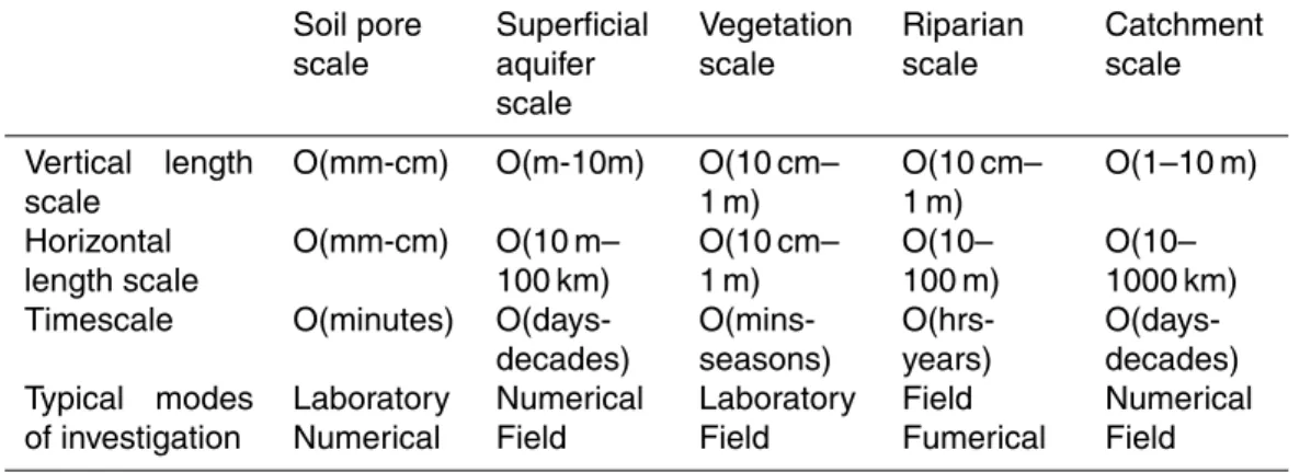
2003a), yet our ability to predict that export relies on a detailed understanding of both the transport and biogeochemical processing taking place (Hornberger et al., 2001). One of the challenges for the prediction of material transfer through catchments, is the high degree of heterogeneity and its dependence on scale. Dooge (1986) suggested that scaling issues were fundamental to the development of hydrological theory,

specifi-5

cally the development of scaling relations across catchment scales and up-scaling from scale theories. Since that time there has been substantial research on small-scale process-based distributed model descriptions, however the application of these models to large catchments has at times been problematic and the preferred modes of investigation continue to vary across scales (Table 1).

10

In response to this, McDonnell et al. (2007) challenged hydrologists to move “beyond heterogeneity and process complexity” to better facilitate the characterization of catch-ments, however approaches using either an ecological or hydrological lens tend to remain embedded in discipline-specific process complexity. In a study that investigated interactions between vegetation and hydrology, Thompson et al. (2011) highlighted

15

the co-evolution of vegetation and hydrological spatial organization, yet continued to use a hydrological lens, via a water balance approach, to characterize systems across scales. An alternative approach is to adopt a dual lens, in which the focus remains on the dynamic balance between hydrological and ecological processes. Here we focus on material fate as expressed by biogeochemical reactions.

20

In an attempt to identify parameters that resolved the “scale” issue, Vach ´e and Mc-Donnell (2006) flagged that water residence times were integrative and meaningful across all scales, and went on to highlight the challenges in characterizing flow paths, and therefore residence times, that were of relevance to material transport; the resi-dence time is a critical parameter within the dual lens approach. The resiresi-dence time

25

(4)

HESSD

9, 10487–10524, 2012

C. E. Oldham et al.

Title Page

Tables Figures

◭ ◮

Back Close

Full Screen / Esc

Discussion

P

a

per

|

Dis

cussion

P

a

per

|

Discussion

P

a

per

|

Discussio

n

P

a

per

|

2010; McGuire and McDonnell, 2006). All of these authors noted the importance of the residence and transit times for the export of pollutants and biogeochemicals from catchments.

Estimates of characteristic residence times have been used in dimensionless ra-tios (Carleton, 2002; Hornberger et al., 2001; Ocampo et al., 2006) to improve our

5

understanding of catchment hydro-chemical responses and chemical cycling. The di-mensionless Damk ¨ohler number, Da, has been used extensively in the discipline of chemical engineering to classify a system according to the balance between transport and reaction, and is given as

Da=τ_τT

R

(1)

10

where τT is the transport (or residence) timescale and τR is the reaction timescale.

Thus, Da can be considered an important non-dimensional number within the dual lens approach.

Michalak (2000) used Da to characterize the appearance of chemical sorption peaks in simulation experiments. Wehrer and Totsche (2003) used Da to characterize when

15

breakthrough of contaminants took place under non-equilibrium conditions, Ocampo et al. (2006) used Da to explore the removal of nitrate by riparian zones and demon-strated that 50 % nitrate removal occurred when Da<1 and increased to nearly 100 % at Da=2–20. Carleton (2002) used Da to explore residence time distributions in treat-ment wetlands and their impact on contaminant removal. Kurtz and Peiffer (2011) used

20

a Da approach to explore turnover timescales and surface complexation reactions. Given that the Da has been successfully used to characterize the transfer of biogeo-chemicals under a range of transport conditions, and across a range of spatial scales from pores to wetlands and riparian zones, we suggest that Da could be used to char-acterize hydrological elements in a catchment. We note however that by definition the

25

(5)

HESSD

9, 10487–10524, 2012

C. E. Oldham et al.

Title Page

Tables Figures

◭ ◮

Back Close

Full Screen / Esc

Discussion

P

a

per

|

Dis

cussion

P

a

per

|

Discussion

P

a

per

|

Discussio

n

P

a

per

|

The hydrological connectivity/disconnectivity dynamic is a key characteristic of many catchments (Meerkerk et al., 2009; Michaelides and Chappell, 2009; Ocampo et al., 2006; Pringle, 2003a, b) and is considered critical for ecological function, adap-tation and evolution (Klein et al., 2009; Opperman et al., 2010; Pringle, 2003b). Pringle (2003b) noted the variety of definitions of connectivity, used across and within

5

disciplines. In recent years, a commonly used definition is the ability of energy, matter and organisms to transfer within and between elements (for example sub-catchments, riparian zones, wetlands, streams) of the hydrologic cycle (Detty and McGuire, 2010; Pringle, 2003b).

Over the past decade there have been numerous attempts to characterise the

10

connectivity/disonnectivity dynamic, most typically in terms of hydrological (surface and sub-surface pathways) or hydraulic (pathways incorporating a free surface, e.g. streams and wetlands) connectivity (Ali and Roy, 2010; Meerkerk et al., 2009; Michaelides and Chappell, 2009; Tetzla_ffet al., 2007). Even where the connectivity def-inition of Pringle (2003b) has been used previously, conservative transfer of material is

15

usually assumed (i.e. still using a hydrological lens). To our knowledge there have been no attempts in the hydrological literature to characterise connectivity in terms of the ef-fectivenessof transferring energy, matter or organisms. Such a characteristic might be termed “ecohydrological” connectivity and must take into account both the hydrolog-ical/hydraulic transport and the biological and/or chemical fate or processing; such a

20

definition is needed under a dual lens approach. Here we define ecohydrology as the interaction between hydrology and the biosphere, with specific regard to biogeochem-ical processing of material. Multiple elements of the hydrologbiogeochem-ical cycle may be fully connected hydrologically, yet if organisms or material is being removed, or even set-tles under gravity, within a single element, the material transfer is not complete across

25

(6)

HESSD

9, 10487–10524, 2012

C. E. Oldham et al.

Title Page

Tables Figures

◭ ◮

Back Close

Full Screen / Esc

Discussion

P

a

per

|

Dis

cussion

P

a

per

|

Discussion

P

a

per

|

Discussio

n

P

a

per

|

To illustrate our point we present two examples. Firstly, we take the example of Fe(II)-rich anoxic groundwaters being discharged into a well oxygenated stream which then flows into a lake. The groundwater, stream and lake are hydrologically and hydrauli-cally fully connected, however Fe(II) undergoes oxidation on exposure to oxygenated waters, and likely precipitates out as Fe(III) oxide, which may a_ffect the benthic

ecol-5

ogy. The balance between the rate of transport, the rate of Fe(II) oxidation, the rate of precipitation and settling, and the rate of Fe(II) production from reductive dissolution, will determine the e_ffectiveness of ecohydrological connectivity, with respect to Fe(II), of the groundwater and lake. If all Fe(II) is oxidized before reaching the lake, the system is ecohydrologically disconnected with respect to Fe(II). Secondly, we take the

exam-10

ple of a phytoplankton-rich wetland being flushed out across a floodplain and into a lake under flooding conditions. The wetland, the floodplain and the lake are hydrauli-cally fully connected, however in transit the phytoplankton may grow, aggregate, settle and decompose. The balance between the rate of transport, the rate of particle settling under gravity and the phytoplankton net productivity will determine the effectiveness

15

of ecohydrological connectivity, with respect to the phytoplankton, of the wetland and the lake. If all phytoplankton settle out (or decompose) before reaching the lake, the system is ecohydrologically disconnected with respect to phytoplankton.

This paper seeks to develop a framework that could be used to conceptually classify ecohydrological systems, including systems undergoing intermittent connectivity, and

20

thus provide insights into processes controlling the export of material from catchments. For clarity, we modify the broader connectivity definition of Pringle (2003b), to a defini-tion of ecohydrological connectivity asthe ability of matter and biota to transfer within and between elements of the hydrologic cycle, while subject to biogeochemical or bio-logical processing. For simplicity, at this point we have excluded energy transfer from

25

(7)

HESSD

9, 10487–10524, 2012

C. E. Oldham et al.

Title Page

Tables Figures

◭ ◮

Back Close

Full Screen / Esc

Discussion

P

a

per

|

Dis

cussion

P

a

per

|

Discussion

P

a

per

|

Discussio

n

P

a

per

|

2 Conceptual framework

Our definition of ecohydrological connectivity explicitly takes into account the transfer of matter and biota across and between hydrological elements. We therefore begin the development of our framework with the scalar transport equation, or advection-diffusion-reaction (ADR) equation, that describes transport of chemicalB via a

homo-5

geneous fluid (constant density and viscosity) and is given as

∂[B] ∂t =−ui

∂[B] ∂xi +Deff

∂2[B] ∂xi∂xi

−k′[B]

I II III (2)

where [B] is the concentration of chemicalB(mmol m−3

),u_i is the mean velocity in the

i-direction (m s−1

),tis time (s),xi is distance in thei-direction (m),Deff is theeffective

diffusion/dispersion coefficient (m2s−1) and k′

is an appropriate rate constant (s−1)

10

where

τR=1/k

′

. (3)

Note that outside of diffusive boundary layers, D_e_ff is likely to be significantly larger than molecular diffusivity and may describe processes such as turbulent diffusion, bio-turbation or mechanical dispersion. Term I describes advective transport of chemical

15

B, Term II describes Fickian transport of chemicalB, and Term III describes the rate at which chemicalBis consumed.

The non-dimensional Peclet Number, Pe, provides the balance between advection and diffusion:

Pe= Deff

u_i∆x_i (4)

20

(8)

HESSD

9, 10487–10524, 2012

C. E. Oldham et al.

Title Page

Tables Figures

◭ ◮

Back Close

Full Screen / Esc

Discussion

P

a

per

|

Dis

cussion

P

a

per

|

Discussion

P

a

per

|

Discussio

n

P

a

per

|

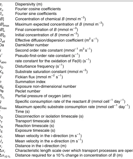
The choices of appropriate control volume, and their relevant time and length scales are critical. A first assumption is that the control volume and therefore the characteristic length scale, ∆x_i, are physically constrained, typically by catchment/stream/wetland geomorphology. The relevant transport timescale,τT, is then determined by the length

scale and the transport process, whether advective or di_ffusive controlled (Fig. 1).

5

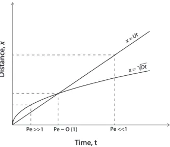
We apply Eq. (2) to an idealized one dimensional control volume or hydrological element (Fig. 2a), which has a physically constrained horizontal length scale of ∆x_i, with through-flow velocityui and effective diffusivityDeff. The general solution to Eq. (2)

is

[B]=exp(−k′t)

"

α0+

∞

X

n=0

αncos

_nπ ∆xi

(x−u_it)

10

+β_nsin

_nπ

∆x_i(x−uit)

exp −n 2

π2Deff

∆x_i2 t

!#

(5)

wherenis the summation index andαnandβnare Fourier cosine and sine coefficients

respectively and are determined by the initial and boundary conditions that apply to the particular element being modeled.

Chemical reaction timescales 15

We have illustrated above the use of Pe to determine the appropriate transport or res-idence timescales, and we now address the estimation of appropriate chemical reac-tion timescales. While acknowledging that many biogeochemical processes have more complex kinetics, for simplicity we initially assume our chemical reaction of interest can be described as

20

(9)

HESSD

9, 10487–10524, 2012

C. E. Oldham et al.

Title Page

Tables Figures

◭ ◮

Back Close

Full Screen / Esc

Discussion

P

a

per

|

Dis

cussion

P

a

per

|

Discussion

P

a

per

|

Discussio

n

P

a

per

|

Equation (6) can be treated as a second order reaction wherek is the second order rate constant (mmol−₁

m3 s−₁

) and if we assumeAto be in excess ofB then Eq. (6) can then be considered “pseudo-first-order” with respect toB, [B] is not limiting and d[B]

dt =−k[A][B]. (7)

The square brackets denote the chemical concentration (mmol m−3

) and k′

is the

5

pseudo-first-order rate constant (s−₁

) and is used in (2).

Alternatively, if we use a Monod model (Park and Jaffe, 1995; Lendenmann and Egli, 1998; Castillo et al., 1999), the rate of consumption of chemicalBcan be parameterized as

d[B]

dt =−q[A] (8)

10

whereqis the specific consumption rate of the reactantB(mmol cell−₁

day−₁

), and the characteristic timescale of reaction,τRis given by Simpson and Landman (2007) as

τR=

[B]max qmax

(9)

where [B]_maxis the maximum expected concentration ofBandk′

=1/τ_R.

Using this conceptual framework, we define three regimes, depending on the relative

15

balances between Terms I, II and III in Eq. (2), and present a modified Eq. (5) for each regime.

2.1 Regime I: advection dominated

For systems that are hydraulically or hydrologically connected and Pe≪1 (i.e. the

system is advection dominated, Fig. 2. Term II in Eq. (2) drops out, leaving

20

∂[B]

∂t =−ui ∂

[B] ∂x_i −k

′

[B]

(10)

HESSD

9, 10487–10524, 2012

C. E. Oldham et al.

Title Page

Tables Figures

◭ ◮

Back Close

Full Screen / Esc

Discussion

P

a

per

|

Dis

cussion

P

a

per

|

Discussion

P

a

per

|

Discussio

n

P

a

per

|

The relevant (advective) transport timescale for this regime is

τ_TA=∆x

U_x (11)

whereU_x is the mean velocity (m s−1

) in thex-direction.

Substituting Eqs. (11) and (3) into Eq. (4) gives the appropriate Damk ¨ohler number for Regime I as

5

Da_I=k

′

∆x

U_x , (12)

When Da≫1,τ_T≫τ_Rwhich indicates that the control volume residence time is suffi

-ciently long for chemicalsAandBto react. When Da≪1,τ_T≪τ_Rwhich indicates that

chemicalsAandBdo not have sufficient time come to react before they are advected out of the control volume; in this case chemicalsAandBmay be treated as if they are

10

conservative. Some examples of environments where we expect of Regime I to occur are shown in Fig. 2.

In the small Pe limit, the diffusion term can be neglected and the general solution Eq. (5) can be re-written as

[B]=exp(−k′t)f(x−ut) (13) 15

where the functionf(x) represents the initial (t=0) distribution of [B] in the element. Physically, as time increases the initial profile of [B] is advected at speeduthrough the element without change of form except for a reduction in magnitude due to the reaction term.

This solution and its behavior are shown in Fig. 4a and b. Figure 4a shows the case

20

where there is no significant consumption ofB (Da≪1) before it has been advected

(11)

HESSD

9, 10487–10524, 2012

C. E. Oldham et al.

Title Page

Tables Figures

◭ ◮

Back Close

Full Screen / Esc

Discussion

P

a

per

|

Dis

cussion

P

a

per

|

Discussion

P

a

per

|

Discussio

n

P

a

per

|

has been a significant reduction of magnitude in the profile. Note however thatB has not spread within the element since this is the advection-dominated regime (i.e. di_ff u-sion is minimal).

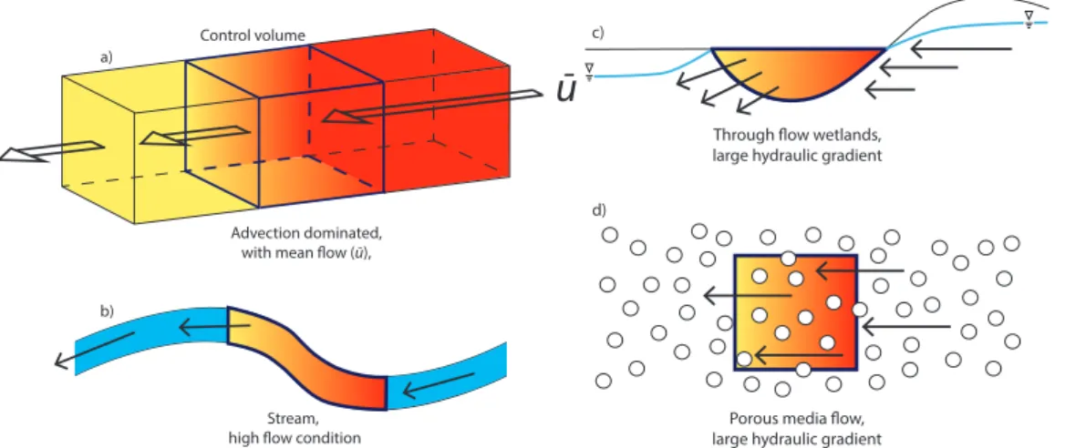
2.2 Regime II: di_ffusion dominated

For systems that are hydraulically or hydrologically connected and Pe≫1 (i.e. system 5

is diffusion dominated, Fig. 3, Term I in Eq. (2) drops out so we have

∂[B] ∂t =Deff

∂2[B] ∂xi∂x)i

−k′[B],

II III (14)

The relevant (diffusive) transport timescale,τ_TD, for this regime is then

τ_TD=∆x

2 i Deff

. (15)

and given Eq. (7), then

10

DaII= k′

∆x2 Deff

(16)

where DaIIis the definition of Da appropriate for this regime.

When Pe≫1 the general solution Eq. (5) can be re-written as

[B]=exp(−k′t)

"

α0+

∞

X

n=0

αncos

_nπ ∆xi

x

+β_nsin

_nπ ∆x_ix

exp −n 2

π2Deff

∆x2_i t

!#

(17)

(12)

HESSD

9, 10487–10524, 2012

C. E. Oldham et al.

Title Page

Tables Figures

◭ ◮

Back Close

Full Screen / Esc

Discussion

P

a

per

|

Dis

cussion

P

a

per

|

Discussion

P

a

per

|

Discussio

n

P

a

per

|

In the absence of significant reaction ofB (Da≪1), B will eventually diffuse through

the entire system without significant loss ofB. This is shown in Fig. 4c. Alternatively, if Da≫1 then much of B will be used up before it has a chance to diffuse through the

system, which is shown in Fig. 4d.

2.3 Regime I and II boundary

5

We have shown how to use Pe and Da to classify eco-hydrological systems, however porous media are frequently characterized by their dispersivity,

αi = Deff

u_i . (18)

If we normalize the dispersivity by the characteristic length scale (i.e. the length of the control volume), then

10

αi

∆x_i = De_ff

u_i∆x_i =Pe. (19)

Note that this relationship is dependent on scale and the empirically derived relation-ship

α_i =0.0175∆x_i1.46 (20)

can be applied to a flow path length less than 3500 m (Todd and Mays, 2005).

15

Reported horizontal field dispersivities considered of high reliability, typically range from 10−2

to 102m, over length scales ranging from 100to 103 m (Gelhar 1992), and using Eq. (18) we get Pe numbers O(10−3)–O(1), indicating that both advection and diffusion are significant in the development of [B] at the upper end of the range. Under this condition, advection and diffusion act on similar time scales.

(13)

HESSD

9, 10487–10524, 2012

C. E. Oldham et al.

Title Page

Tables Figures

◭ ◮

Back Close

Full Screen / Esc

Discussion

P

a

per

|

Dis

cussion

P

a

per

|

Discussion

P

a

per

|

Discussio

n

P

a

per

|

2.4 Regime III – hydrological disconnection

We have shown how to use Pe and Da to classify ecohydrological systems, however so far we have assumed hydrological/hydraulic connectivity. In temperate, semi-arid and arid environments, there may be times when elements of the hydrological cycle are hydrologically or hydraulically disconnected. During these periods, chemical and

5

biological reactions continue within the hydrological element and biogeochemicals will accumulate or decline, creating an isolated biogeochemical reactor in the environment. Under these conditions

∂[B]

∂t =−k

′

[B] (21)

The general solution Eq. (5) can then be re-written simply as

10

[B]₌exp(k′

t)f(x) (22)

wheref(x) is the initial (t=0) distribution of [B].

Examples of aquatic systems that are hydrologically or hydraulically disconnected are shown in Fig. 5. We can assume full internal mixing of these systems due to exter-nal forcing (e.g. due to wind mixing).

15

If we take the reaction shown in Eq. (6) then the extent to which chemical B is re-moved is determined by both rate of reaction and also the timescale over which the hydrological element is physically disconnected or isolated. We will call this the isola-tion timescale, τ_I. When hydrological elements become isolated with no water fluxes in or out, the chemical reaction shown in Eq. (6) may quickly become limited by either

20

the depletion of reactants or the build up of products. The consequences of hydrologi-cal/hydraulic isolation are no resupply of reactants and no flushing of products. Under these conditions, the change in concentration ofBcannot be described by Eq. (7) and we should instead use Eq. (8), however to illustrate our conceptual framework we will assume that until chemical B is 10 % consumed, pseudo-first order kinetics can be

25

(14)

HESSD

9, 10487–10524, 2012

C. E. Oldham et al.

Title Page

Tables Figures

◭ ◮

Back Close

Full Screen / Esc

Discussion

P

a

per

|

Dis

cussion

P

a

per

|

Discussion

P

a

per

|

Discussio

n

P

a

per

|

We now present a new non-dimensional number to describe this Regime III as the ratio of residence or isolation timescale to reaction timescale

NIII= τI τR

(23)

If we take the inverse of the isolation timescale, τI, we obtain what we can term the

hydrological/hydraulic connection frequency. Alternatively if the isolated system itself

5

is the reference point then 1/τIis the disturbance frequency,kD, a concept used

exten-sively in terrestrial ecology (Huston, 1994).

3 Discussion

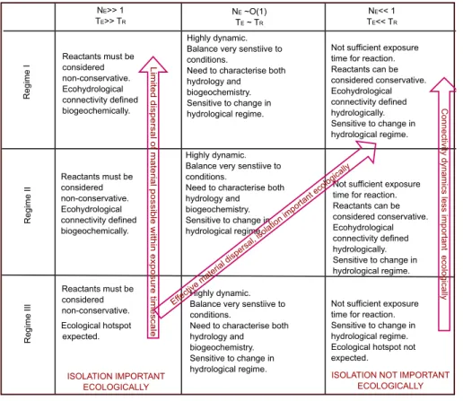
3.1 Non-dimensional numbers

The Damk ¨ohler number has been used extensively in chemical engineering and more

10

recently in environmental and hydrological contexts and we have shown above that it provides a useful classification of eco-hydrological systems. However, the definition of Da implicitly assumes hydrological or hydraulic connectivity. Without physical connec-tivity, there is no transport of chemicals across hydrological elements, therefore we are unable to defineτT. For example Da could not be used to describe Regime III, where 15

we defined the system in terms of the timescale of isolation,τ_I. A new non-dimensional number, NIII was created to account for this constraint. It should be noted that NIII

does not characterize material connectivity, but rather the potential for material to be disbursed once hydrological connectivity is again established. This potential for dis-bursal has significant implications for both small-scale and landscape-scale ecological

20

processes, as will be discussed below.

(15)

HESSD

9, 10487–10524, 2012

C. E. Oldham et al.

Title Page

Tables Figures

◭ ◮

Back Close

Full Screen / Esc

Discussion

P

a

per

|

Dis

cussion

P

a

per

|

Discussion

P

a

per

|

Discussio

n

P

a

per

|

number

NE= τE τR

(24)

whereτEis an exposure timescale. This is the timescale over which the

biogeochem-icals or materials have the opportunity to be processed. This opportunity may occur during transport (whenτE=τT andNE=Da i.e. Regimes I and II depending on Pe) or 5

during hydrological/hydraulic isolation (whenτE=τI andNE=NIIIi.e. Regime III). The

concept of an exposure timescale has been previously used in surface renewal the-ory (Dankwerts, 1951) and chemical engineering (Asarita, 1967). The proposed non-dimensional number therefore gives an indication of the extent of chemical reaction possible within the exposure timescale.

10

NEcan be used to determine the physical constraints on a system required to ensure,

for example, that 90 % of a biogeochemical is removed. If we take the example of a pseudo-first-order reaction as shown in Eq. (6) and our definition shown in Eq. (23) then Eq. (7) can be integrated to obtain

[B]∗=[B]0exp(−k ′

τE) 15

=[B]₀exp(−N_E). (25)

When chemicalBis 90 % removed, [B]∗

[B]0

=0.1=exp(−N_E) (26)

thenN_E≈2.3. So for a system whereN_E≫2.3, we expect more than 90 % removal of

chemical. For a system whereNE≪2.3, we expect less than 90 % removal of chemi-20

cal. If we are aiming for biogeochemical removal, for example in reconstructed riparian zones, we could manipulate the physical system to ensure we have N_E≫2.3, and

thus achieve at least 90 % removal. We can thus use the concept ofNEto identify the

required timescale, and then with knowledge of the transport mechanisms, physically size the system to ensure the opportunity timescale is appropriate. Similarly we use

25

(16)

HESSD

9, 10487–10524, 2012

C. E. Oldham et al.

Title Page

Tables Figures

◭ ◮

Back Close

Full Screen / Esc

Discussion

P

a

per

|

Dis

cussion

P

a

per

|

Discussion

P

a

per

|

Discussio

n

P

a

per

|

3.2 Application of Pe/Da approach across scales

In the previous sections we outlined how Da and Pe can be used to classify eco-hydrological systems according to the fate of chemical B. We will now examine this concept for several hydrological systems across different temporal and spatial scales. We will focus on the oxidation of Fe(II) which plays a prominent role in linking metabolic

5

activities across anaerobic and aerobic components of aquatic systems (Raiswell and Canfield, 2012). Fe(II) oxidation is an ecologically significant reaction both under neu-tral and acidic conditions however the rate is strongly dependent on pH (Stumm and Morgan, 1996). The oxidation process typically implies precipitation of ferric oxides and through that the generation of acidity. Under well-bu_ffered conditions, such as

anaero-10

bic ground or pore waters, the pH remains relatively constant. Under low or no-alkalinity conditions however, oxidation of Fe(II) significantly contributes to acidification of surface waters. Examples of such systems are acidic mining lakes (Peine et al., 2000) or acid sulphate soils (Burton et al., 2006) where acidity has been generated through the oxi-dation of pyrite, but where acidic iron cycling i.e. the combined reduction of ferric and

15

oxidation of ferrous iron, maintains acidic conditions (Peine et al., 2000). Here we will compare three anaerobic aquatic systems containing Fe(II) and how they respond to oxygen exposure under different transport regimes. We have chosen two pH condi-tions: neutral (pH 7) conditions as found in many anaerobic environments, and slightly acidic (pH 4) conditions as found in many anaerobic systems receiving waters that

20

have been exposed to pyrite oxidation (Blodau, 2006).

The oxidation of Fe(II) can be modelled using the rate law given by Stumm and Lee (1961).

d[Fe(II)]

dt =−kabioPO2[OH

−

]2[Fe(II)] (27)

wherePO₂ is the partial pressure of oxygen (0.21 atm) and kabio is the rate constant 25

(17)

HESSD

9, 10487–10524, 2012

C. E. Oldham et al.

Title Page

Tables Figures

◭ ◮

Back Close

Full Screen / Esc

Discussion

P

a

per

|

Dis

cussion

P

a

per

|

Discussion

P

a

per

|

Discussio

n

P

a

per

|

This rate law predicts extremely low rates under acidic conditions. Typically, Fe(II) oxidation will be accelerated by bacteria. Pesic et al. (1989) reported a decrease in microbial oxidation rate with increasing pH between pH 2.2 and pH 3. Extrapolation of their rate law (Kirby et al., 1999) demonstrates that at pH 4 the abiotic rate is still higher then the microbial rate. Hence, in our examination we will use Eq. (26) for pH 4 and pH

5

7.

The rate constantk in Eq. (26) can be converted into a pseudo 1st-order rate con-stant for ambient temperature and pressure conditions and for a pre-defined pH as

k′

=kabioPO₂[OH

−

]2 (28)

10

which yields the reaction times,τR, given in Todd and Mays (2005), that will be used

for the analyses below.

3.3 Case I: porewater transport in deep lake sediments

The sediment of deep eutrophic lakes (pH neutral conditions) or mining lakes (acidic conditions) may be hydrologically connected to the surrounding groundwater but if the

15

hydraulic conductivity of the sediment material is extremely low, groundwater inflow velocities could be<10−₉

m s−₁

. We assume a molecular di_ffusion coe_fficient,Deff of

10−9

m2s−

1.

Under this scenario, the characteristic length scale is not physically constrained. We can, however, estimate a depth at which the O₂ concentration has been

de-20

creased to a specified level. In order to fulfil the validity of pseudo-first order kinet-ics we assume a reduction by only 10 %, i. e.∆PO₂=0.021 atm which corresponds to

∆[O₂]≈0.03 mol l−1 at ambient temperature, and stoichiometrically to an Fe(II)

con-sumption of∆[FeII]=0.03 mol l−1. Hence, the thickness of a layer will be estimated, in which the oxygen concentration does not drop below 0.27 mol l−1

.

25

Fe(II) concentrations in pH neutral lake sediments rarely exceed 0.1 mol l−1

(18)

HESSD

9, 10487–10524, 2012

C. E. Oldham et al.

Title Page

Tables Figures

◭ ◮

Back Close

Full Screen / Esc

Discussion

P

a

per

|

Dis

cussion

P

a

per

|

Discussion

P

a

per

|

Discussio

n

P

a

per

|

mmol l−1

may be reached (Burton et al., 2006; Peine et al., 2000). Therefore, a∆[FeII] of 0.03 mol l−1

is a 30 % removal at pH 7 and a 0.3 % removal at pH 4. Using Eq. (25),

NE≈0.4 and 0.003 for pH 7 and 4 respectively.

In the next step we can estimate∆x10 %by combining Eqs. (15) and (23) as

∆x10 %=

q

NE×τr×Deff (29)

5

which yields 8×10−4m at pH 7, and 8×10−2m at pH 4. The corresponding exposure

timescales,τE, within these contact zones are 7×10 2

s at pH 7, and 6×106s at pH

4. Using these length scales, groundwater inflow velocities and molecular diffusion coefficient, Pe ranges from 1.2×103at pH 7 to 1.3×101at pH 4 (Table 3).

The above calculations have two specific implications. Firstly, the thickness of the

10

layer that remains close to O2 saturation varies significantly between the two pH

regimes. The zone of of Fe(II) production from dissimilatory iron reduction (a biogeo-chemical process sensitive to O₂) will be shifted to deeper sediments under acidic conditions. Secondly and more importantly, the timescales of exposure to oxygen sat-uration is 4 orders of magnitudes longer under acidic conditions and lasts for several

15

weeks. Note that the calculated τE is an lower estimate and may be even longer at

lower Fe(II) concentrations. This long time scale provides ample opportunities for inter-ference from other biogeochemical processes that involve oxygen or consume Fe(II).

Hence, N_Ecan be regarded as a process-specific parameter that allows us to classify ecohydrological systems based on chemical fate. When NE∼O(1), as was calculated 20

under pH 7, the balance between transport and reaction is critical and the system will be sensitive to shifts in hydrological regime. When N_E≪O(1), as was calculated under

pH 4, the system will not be sensitive to shifts in hydrological regime.

3.4 Case II: surface water – groundwater exchange

The advective recharge of oxygenated surface waters into Fe(II)-rich groundwater is

25

(19)

HESSD

9, 10487–10524, 2012

C. E. Oldham et al.

Title Page

Tables Figures

◭ ◮

Back Close

Full Screen / Esc

Discussion

P

a

per

|

Dis

cussion

P

a

per

|

Discussion

P

a

per

|

Discussio

n

P

a

per

|

majority of these systems are pH neutral, wetlands affected by acid sulphate soils (Johnston et al., 2011) and mining lakes (Fleckenstein et al., 2009) may lose acidic water to groundwater.

Again under this scenario, the characteristic length scale is not physically con-strained, so we can estimate the length scales over which the O₂ concentration has

5

been decreased by 10 %. The Fe(II) boundary conditions are selected as in Case I.

∆x10 %can be now calculated by using Eqs. (11) and (23) as

∆x10 %=UxτrNE, (30)

BothNEand exposure timescales,τE, are the same as in case I. However the distance

from the riparian zone over which 10 % of O2 is consumed differs from Case I and is 10

6×10−3m at pH 7, and 5×101m at pH 4. In other words, after 50 m of flow across a

riparian zone at pH 4 the system would still be close to oxygen saturation, allowing O₂ consuming reactions.

To calculate Pe numbers we can use Eq. (18). In porous-media flow,De_ffbecomes a

scale-dependent dispersion coe_fficient, which can be estimated from the dispersivity,α,

15

of the aquifer into which the lake water penetrates; see Eq. (18). We getα_i=1×10−5m

and Deff=1×10

−1

m2s−1

for pH 7 and α_i=6.4 m and Deff=6×10

−5

m2s−1

for pH 4. Thus at pH 7, i.e. within the short distance of 6 mm, no dispersion occurs. The corresponding Pe ranges from 2×10−3at pH 7 (indicating advective transport through

the O2containing layer) to 1.1×10

−1

at pH 4 (indicating some dispersive effects during

20

transport).

3.5 Case III: temporarily disconnected systems

Floodplain wetlands and playas frequently become temporarily disconnected from sur-face and sub-sursur-face water flow pathways. In Western Australia, groundwater-fed wet-lands affected by acid sulphate soils, fill with Fe(II)-rich groundwater which is then

ex-25

(20)

HESSD

9, 10487–10524, 2012

C. E. Oldham et al.

Title Page

Tables Figures

◭ ◮

Back Close

Full Screen / Esc

Discussion

P

a

per

|

Dis

cussion

P

a

per

|

Discussion

P

a

per

|

Discussio

n

P

a

per

|

the wetlands from the source of Fe(II), and its subsequent oxidation via ongoing expo-sure to O₂is controlled by the disconnection timescale,τD. Depending on the buffering

capacity of the wetland mineralogy, both acidic and neutral conditions can be observed. Under this scenario, the characteristic length and time scales are physically con-strained. If we assume a typicalτD∼100 days (∼10

7

s), then using Eq. (24), we

esti-5

mate the extent of Fe(II) oxidation as 100 % at pH 7 and 1 % at pH 4. The differences between Fe(II) oxidation at the different pHs can also be demonstrated by the non-dimensional number,NE. Using (23),NE is 5×10

3

at pH 7 (indicating the disconnec-tion time scale provides sufficient exposure opportunity for the reaction to proceed) and 5×10−3at pH 4 (indicating that the disconnection time scale does not provide enough 10

time for the reaction to proceed).

Again, NE can be regarded as a process-specific parameter that allows us to

clas-sify ecohydrological systems based on chemical fate. WhenNE≫O(1), as was

cal-culated under pH 7, the system will be sensitive to changes in hydrological regime; any increase in isolation timescale will cause an increase in chemical reaction. When

15

NE≪O(1), as was calculated under pH 4, the system will not be sensitive to shifts in

hydrological regime.

4 Conclusions

4.1 Water management

We have shown that the new non-dimensional number, NE, can be used to classify 20

the ecohydrological systems, their potential for material transfer and their sensitivity to shifts in hydrological regimes.NEcan also be used to calculate the distance of reactive

zones. Extending this idea, Eqs. (28) and (29) can be directly applied for water manage-ment purposes. For example, we propose that the width of a riparian zone in which no agricultural activity is allowed, can be calculated using the framework presented here,

25

(21)

HESSD

9, 10487–10524, 2012

C. E. Oldham et al.

Title Page

Tables Figures

◭ ◮

Back Close

Full Screen / Esc

Discussion

P

a

per

|

Dis

cussion

P

a

per

|

Discussion

P

a

per

|

Discussio

n

P

a

per

|

width might correspond to the lengthscale, ∆x, that is required to remove e.g. 90 % of the nitrate that has infiltrated to groundwater from agricultural land. To some extent the “50 day-line” typically applied to constrain drinking water zones implicitly uses this concept already.

4.2 Competiveness of reactions

5

We have shown thatNEnumbers are reaction specific; the corresponding spatial scales

are also reaction dependent and not necessarily controlled by geomorphology. In a first approach, we can therefore argue that lowNEimplies ample opportunity for other

reactions to proceed within a certain hydrological element. Inversely, highNE implies

predominance of the biogeochemical process of interest.NEis thus a reaction-specific 10

parameter that allows us to compare the effectiveness of different material processing reactions across a certain temporal (τE) or spatial (∆x) scale.

More generally, lowerNEimplies a lower competiveness of a specific reaction. In the

examples discussed above, the oxidation of Fe(II) is much more competitive at pH 7 than at pH 4. In this case competiveness is clearly controlled by the large differences

15

ink′

. However,NEis of course also affected by the exposure timescale. We therefore

propose that for a given system,NE can be used as a general parameter to compare

competiveness between different reactions of interest.

Competiveness of redox reactions is typically discussed in terms of thermodynamic arguments, for example the gain in free energy,∆Gf, obtained from oxidation of organic 20

matter (Huston, 1994). This concept works very well in diffusion controlled systems such as the sediment porewaters of the ocean or deep lakes. Attempts to adapt this concept to groundwater systems have been problematic. Rather, zones of intensive redox activity are observed to be spatially distributed or located at plume fringes (see e.g. Prommer et al., 2006). Considering that the rate of a reaction is proportional to

25

∆Gf, thermodynamics is also related to the reaction timescale. Considering further that

(22)

HESSD

9, 10487–10524, 2012

C. E. Oldham et al.

Title Page

Tables Figures

◭ ◮

Back Close

Full Screen / Esc

Discussion

P

a

per

|

Dis

cussion

P

a

per

|

Discussion

P

a

per

|

Discussio

n

P

a

per

|

then it becomes clear that∆Gf and NE are interrelated predictors for competiveness

under di_ffusion-controlled (or well-mixed) conditions.

Under advection or dispersion controlled conditions however, the timescale of expo-sure along a flow path, i.e. the expoexpo-sure spatial scale, varies strongly depending on external forcing. Of course the flow paths and therefore exposure timescales may be

5

distributed in space, similar to residence times, and this spatial variability will give rise to a patchwork ofNE values, paralleling the concept of “residence time distributions”,

with each controlled by specific biogeochemical regimes. Under these conditions, as for diffusion-controlled conditions, chemical competiveness becomes dependent on the exposure time; NE therefore can be used as a general parameter to compare com-10

petiveness under all regimes.

4.3 Ecological consequences

Hydrological systems transition, according to external forcing, between two or three of the regimes outlined above. In particular, systems in Regime III, i.e. the disconnected state, will intermittently transition to Regime I and/or II. Estimates of NE for Regime 15

III systems when compared toNEfor their hydrologically connected counterparts,

pro-vide a framework for predicting the biogeochemical and ecological significance of the disconnection period (Table 4).

An example of transition between regimes is the drying and re-wetting cycles in-duced by oscillating groundwater tables. Typically these cycles are accompanied by

20

transitions between anoxic and oxic conditions, and changes in biogeochemical bound-aries. One consequence of such cycling would be the export of products under a high groundwater table (Regime I or II) that have accumulated under a lowering groundwa-ter table (Regime III). We speculate that the extent to which a system is resilient to such transitions is likely controlled by the relative rates at which a microbial community can

25

respond to environmental change or disturbance (i.e.k′

(23)

HESSD

9, 10487–10524, 2012

C. E. Oldham et al.

Title Page

Tables Figures

◭ ◮

Back Close

Full Screen / Esc

Discussion

P

a

per

|

Dis

cussion

P

a

per

|

Discussion

P

a

per

|

Discussio

n

P

a

per

|

accumulated reactants can be expected to be beneficial in preventing export of such products.

So far we have constrained ourselves to considering specific biogeochemical re-actions occurring within and across elements of the hydrological cycle. Finally, we broaden our focus to consider landscape-scale ecological processes and their

char-5

acteristic time scales. If we set the biogeochemical rate,k′

, to be analogous to popu-lation growth rate and the isopopu-lation timescale,τI, to be analogous to the reciprocal of

the disturbance frequency then the two timescales in Regime III, see Eq. (22), have direct analogues to concepts in terrestrial ecology. The ratio of the population growth rate and the disturbance frequency, i.e. NE in our framework, impacts on biodiversity 10

and ecological resilience (Huston, 1994).

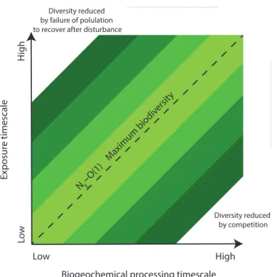
Of particular interest is the conceptual understanding that community biodiversity is maximal when there is a balance between population growth rate (or biogeochemical reaction rate) and disturbance frequency, i.e. whenNE∼O(1) (Fig. 6). The biodiversity

in turn affects ecosystem resilience (Gunderson, 2000; Scheffer and Carpenter, 2003)

15

however the stability space within which ecosystem resilience operates is determined by external factors, and has been related to characteristic spatial or temporal scales of external forcing (Scheffer and Carpenter, 2003). We have shown above that NE

are process specific so the question arises whether we can describe the resilience of a system in terms of itsNE distribution. We speculate that highest resilience may 20

be expected under conditions where all processes operate at comparableNE values,

i.e. mean value ofNE,i ∼O(1).

Acknowledgements. The authors would like to express thanks to a large number of people who over the years have contributed to lively discussion on the use of Da and other non-dimensionless numbers for characterizing catchments, including Carlos Ocampo, Murugesu

25

(24)

HESSD

9, 10487–10524, 2012

C. E. Oldham et al.

Title Page

Tables Figures

◭ ◮

Back Close

Full Screen / Esc

Discussion

P

a

per

|

Dis

cussion

P

a

per

|

Discussion

P

a

per

|

Discussio

n

P

a

per

|

References

Ali, G. A. and Roy, A. G.: Shopping for hydrologically representative connectivity metrics in a humid temperate forested catchment, Water Resour. Res., 46, 1–24, doi:10.1029/2010WR009442, 2010.

Asarita, G.: Mass transfer and chemical reactions, Elsevier Amsterdam, 1967.

5

Bevan, K. J.: Rainfall-runoffmodelling: The primer, Wiley, New York, 2001.

Blodau, C.: A review of acidity generation and consumption in acidic coal mine lakes and their watersheds, Sci. Total Environ., 369, 307–332, 2006.

Botter, G., Bertuzzo, E., and Rinaldo, A.: Catchment residence and travel time distributions: The master equation, Geophys. Res. Lett., 38, 1–6, doi:10.1029/2011GL047666, 2011.

10

Burton, E., Bush, R., and Sullivan, L.: Sedimentary iron geochemistry in acidic waterways as-sociated with coastal lowland acid sulfate soils, Geochim. Cosmochim. Acta, 79, 5455–5468, 2006.

Carleton, J. N.: Damkohler number distributions and constituent removal in treatment wetlands, Ecol. Eng., 19, 233–248, 2002.

15

Dankwerts, P. V.: Absorption by simultaneous di_ffusion and chemical reaction into particles of various shapes and into falling drops, T. Faraday Soc., 47, 1014–1023, 1951.

Detty, J. M. and McGuire, K. J.: Topographic controls on shallow groundwater dynamics: im-plications of hydrologic connectivity between hillslopes and riparian zones in a till mantled catchment, Hydrol. Process., 24, 2222–2236, doi:10.1002/hyp.7656, 2010.

20

Dooge, J. C. I.: Looking for hydrologic laws, Water Resour. Res., 22, 6W0295, doi:10.1029/WR022i09Sp0046S, 1986.

Fleckenstein, J., Neumann, C., Volze, N., and Beer, J.: Raumzeitmuster des Grundwasser-Seeaustausches in einem Tagebaurestsee, Grundwasser, 14, 207–217, 2009.

Gelhar, L. W., Welty, C., and Rehfeldt, K. R.: A critical review of data on field-scale dispersion

25

in aquifers, Water Resour. Res., 28, 1955–1974, 1992.

Gunderson, L. H.: Ecological resilience - in theory and application, Annu. Rev. Ecol. Syst., 31, 425–439, 2000.

Hornberger, G. M., Scanlon, T. M., and Raffensperger, J. P.: Modelling transport of dissolved silica in a forested headwater catchment: the effect of hydrological and chemical time scales

30

(25)

HESSD

9, 10487–10524, 2012

C. E. Oldham et al.

Title Page

Tables Figures

◭ ◮

Back Close

Full Screen / Esc

Discussion

P

a

per

|

Dis

cussion

P

a

per

|

Discussion

P

a

per

|

Discussio

n

P

a

per

|

Hrachowitz, M., Soulsby, C., Tetzlaff, D., Malcolm, I. A., and Schoups, G.: Gamma distribu-tion models for transit time estimadistribu-tion in catchments: Physical interpretadistribu-tion of parameters and implications for time-variant transit time assessment, Water Resour. Res., 46, W10536, doi:10.1029/2010WR009148, 2010.

Huston, M. A.: Biological diversity: The coexistence of species on changing landscapes,

Cam-5

bridge University Press: Cambridge, 1994.

Johnston, S., Keene, A., Bush, R., Sullivan, L., and Wong, V.: Tidally driven water column hydro-geochemistry in a remediating acidic wetland, J. Hydrol., 409, 128–139, 2011. Kirby, C., Thomas, H., Southam, G., and Donald, R.: Relative contributions of abiotic and

bio-logical factors in Fe(II) oxidation in mine drainage, Appl. Geochem., 14, 511–530, 1999.

10

Klein, C., Wilson, K., Watts, M., Stein, J., Berry, S., Carwardine, J., Smith, M. S., Mackey, B., and Possingham, H.: Incorporating ecological and evolutionary processes into continental-scale conservation planning, Ecological applications?, Ecological Society of America, 19, 206–17, 2009.

Kurtz, W. and Peiffer, S.: The role of transport in aquatic redox chemistry, in: Aquatic redox

15

chemistry, 2011.

Lendenmann, U. and Egli, T.: Kinetic models for the growth of Escherichia coli with mixtures of sugars under carbon-limited conditions, Biotechnol. Bioeng., 59, 99–107, 1998.

McDonnell, J.J, McGuire, K., Aggarwal, P., Beven, K. J., Biondi, D., Destouni, G., Dunn, S., James, A., Kirchner, J., Kraft, P., Lyon, S., Maloszewski, P., Newman, B., Pfister, L., Rinaldo,

20

A., Rodhe, A., Sayama, T., Seibert, J., Solomon, K., Soulsby, C., Stewart, M., Tetzlaff, D., To-bin, C., Troch, P., Weiler, M., Western, A., W ¨orman, A., and Wrede, S.: How old is streamwa-ter? Open questions in catchment transit time conceptualization, modelling and analysis, Hydrol. Process., 24, 1745–1754, doi:10.1002/hyp.7796, 2010.

McDonnell, J. J., Sivapalan, M., Vach ´e, K., Dunn, S., Grant, G., Haggerty, R., Hinz, C., Hooper,

25

R., Kirchner, J., Roderick, M. L., Selker, J., and Weiler, M.: Moving beyond heterogeneity and process complexity: A new vision for watershed hydrology, Water Resour. Res., 43, 1–6, doi:10.1029/2006WR005467, 2007.

McGuire, K. and McDonnell, J.: A review and evaluation of catchment transit time modeling, J. Hydrol., 330, 543–563, doi:10.1016/j.jhydrol.2006.04.020, 2006.

30

(26)

HESSD

9, 10487–10524, 2012

C. E. Oldham et al.

Title Page

Tables Figures

◭ ◮

Back Close

Full Screen / Esc

Discussion

P

a

per

|

Dis

cussion

P

a

per

|

Discussion

P

a

per

|

Discussio

n

P

a

per

|

Michaelides, K. and Chappell, A.: Connectivity as a concept for characterising hydrological be-haviour Definitions of Connectivity, Hydrol. Process., 522, 517–522, doi:10.1002/hyp.7214, 2009.

Michalak, A. and Kitanidis, P.: Macroscopic behavior and random-walk particle tracking of ki-netically sorbing solutes, Water Resour. Res., 36, 2133–2146, doi:10.1029/2000WR900109,

5

2000.

Nath, B., Lillicrap, A., Ellis, L., Boland, D., and Oldham, C.: Seasonal hydrological connectivity across an acidic coastal wetland and its impact on contaminant discharge to downstream waterways, Water Resour. Res., under review, 2012.

Ocampo, C. J., Oldham, C. E., and Sivapalan, M.: Nitrate attenuation in agricultural

catch-10

ments: Shifting balances between transport and reaction, Water Resour. Rese., 42, 1–16, doi:10.1029/2004wr003773, 2006.

Opperman, J. J., Luster, R., McKenney, B. A., Roberts, M., and Meadows, A. W.: Ecologically Functional Floodplains: Connectivity, Flow Regime, and Scale, J. Am. Water Resour. Assoc., 46, 211–226, doi:10.1111/j.1752-1688.2010.00426.x, 2010.

15

Park, S. S. and Jaffe. P. R.: Development of a sediment redox potential model for the assess-ment of post-depositional metal mobility, Ecol. Modell., 91, 169–181, 1995.

Peine, A., Kusel, K., Tritschler, A., and Peiffer, S.: Electron flow in an iron-rich acidic sediment – evidence for an acidity-driven iron cycle, Limnol. Oceanogr., 45, 1077–1087, 2000. Pesic, B., Oliver, D., and Wichlacz, P.: An electrochemical method of measuring the oxidation

20

rate of ferrous to ferric iron with oxygen in the presence of Thiobacillus ferrooxidans, Biotech-nol. Bioeng., 33, 428–439, 1989.

Pringle, C.: The need for a more predictive understanding of hydrologic connectivity, Aquatic Conservation: Marine and Freshwater Ecosystems, 13, 467–471, doi:10.1002/aqc.603, 2003a.

25

Pringle, C.: What is hydrologic connectivity and why is it ecologically important?, Hydrol. Pro-cess., 17, 2685–2689, doi:10.1002/hyp.5145, 2003b.

Prommer, H., Tuxen, N., and Bjerg, P.: Fringe-controlled natural attenuation of phenoxy acids in a landfill plume: integration of field-scale processes by reactive transport modeling, Environ. Sci. Technol., 40, 4732–4738, 2006.

30

(27)

HESSD

9, 10487–10524, 2012

C. E. Oldham et al.

Title Page

Tables Figures

◭ ◮

Back Close

Full Screen / Esc

Discussion

P

a

per

|

Dis

cussion

P

a

per

|

Discussion

P

a

per

|

Discussio

n

P

a

per

|

Scheffer, M. and Carpenter, S. R.: Catastrophic regime shifts in ecosystems: linking theory to observation, Trends Ecol. Evol., 18, 648–656, doi:10.1016/j.tree.2003.09.002, 2003.

Simpson, M. J. and Landman, K. A.: Analysis of split operator methods applied to reactive transport with Monod kinetics, Adv. Water Resour., 30, 2026–2033, doi:10.1016/j.advwatres.2007.04.005, 2007.

5

Stumm, W. and Lee, G.: Oxygenation of Ferrous Iron, Ind. Eng. Chem., 53, 143–146, 1961. Stumm, W. and Morgan, J. J.: Aquatic chemistry: chemical equilibria and rates in natural waters,

John Wiley & Sons, Inc, New York, USA, 1996.

Tetzlaff, D., Soulsby, C., Bacon, P. J., and Youngson, A. F.: Connectivity between landscapes and riverscapes — a unifying theme in integrating hydrology and ecology in catchment

sci-10

ence?, Hydrol. Process., 1389, 1385–1389, doi:10.1002/hyp.6701, 2007.

Thompson, S. E., Harman, C. J., Troch, P. A., Brooks, P. D., and Sivapalan, M.: Spatial scale de-pendence of ecohydrologically mediated water balance partitioning: A synthesis framework for catchment ecohydrology, Water Resour. Res., 47, 1–20, doi:10.1029/2010WR009998, 2011.

15

Todd, D. and Mays, L.: Groundwater Hydrology, John Wiley & Sons, Chichester, 2005.

Vach ´e, K. B. and McDonnell, J. J.: A process-based rejectionist framework for evaluating catch-ment runoff model structure, Water Resour. Res., 42, 1–15, doi:10.1029/2005WR004247, 2006.

Wehrer, M. and Totsche, K. U.: Detection of non-equilibrium contaminant release in soil

20

columns: Delineation of experimental conditions by numerical simulations, J. Plant Nutr. Soil Sc., 166, 475–483, doi:10.1002/jpln.200321095, 2003.

(28)

HESSD

9, 10487–10524, 2012

C. E. Oldham et al.

Title Page

Tables Figures

◭ ◮

Back Close

Full Screen / Esc

Discussion

P

a

per

|

Dis

cussion

P

a

per

|

Discussion

P

a

per

|

Discussio

n

P

a

per

|

Table 1. Different preferred modes of investigation used for different scales of elements in hydrological systems.

Soil pore scale

Superficial aquifer scale

Vegetation scale

Riparian scale

Catchment scale

Vertical length scale

O(mm-cm) O(m-10m) O(10 cm– 1 m)

O(10 cm– 1 m)

O(1–10 m)

Horizontal length scale

O(mm-cm) O(10 m– 100 km)

O(10 cm– 1 m)

O(10– 100 m)

O(10– 1000 km) Timescale O(minutes)

O(days-decades)

O(mins-seasons)

O(hrs-years)

O(days-decades) Typical modes

of investigation

Laboratory Numerical

Numerical Field

Laboratory Field

Field Fumerical

(29)

HESSD

9, 10487–10524, 2012

C. E. Oldham et al.

Title Page

Tables Figures

◭ ◮

Back Close

Full Screen / Esc

Discussion

P

a

per

|

Dis

cussion

P

a

per

|

Discussion

P

a

per

|

Discussio

n

P

a

per

|

Table 2.Pseudo-first order rate constants,k′

, and reaction timescales,τR, for the oxidation of iron(II) under different pH conditions.

pH (min−1

) (s)

The potential for material processing in hydrological systems &ndash; a novel classification approach

HESSD

The potential for material processing

in hydrological systems – a novel

classification approach

HESSD

HESSD

HESSD

HESSD

HESSD

HESSD

HESSD

HESSD

HESSD

HESSD

HESSD

HESSD

HESSD

HESSD

HESSD

HESSD

HESSD

HESSD

HESSD

HESSD

HESSD

HESSD

HESSD

HESSD

HESSD

HESSD

HESSD

HESSD

The potential for material processing in hydrological systems – a novel classification approach