Preliminary report
CHEMICAL POTENTIAL OF A LENNARD JONES FLUID
V. ˇCelebonovi´c
Institute of Physics, Pregrevica 118, 11080 Zemun-Belgrade, Serbia
E–mail: [email protected]
(Received: August 26, 2010; Accepted: November 18, 2010)
SUMMARY: The aim of this paper is to present results of analytical calculation of chemical potential of a Lennard Jones (LJ) fluid performed in two ways: by using the thermodynamical formalism and the formalism of statistical mechanics. The integration range is divided into two regions. In the small distance region, which isr≤σin the usual notation, the integration range had to be cut off in order to avoid the occurence of divergences. In the large distance region, the calculation is technically simpler. The calculation reported here will be useful in all kinds of studies concerning phase equilibrium in a LJ fluid. Interesting kinds of such systems are the giant planets and the icy satellites in various planetary systems, but also the (so far) hypothetical quark stars.
Key words. Equation of state
1. INTRODUCTION
The aim of this paper is to present a calcu-lation of chemical potential of a fluid consisting of neutral atoms or molecules. Interest in such systems has considerably increased towards the end of the last century, as a consequence of progress in planetary science. Until the end of October 2010, according to data at http://exoplanet.eu, as much as 493 planets outside the Solar system have been detected. It has been shown that 423 of them have massesM ≤5MJ
where MJ is the mass of Jupiter. The major part
(398) of the stars with planets have masses equal to or smaller than the solar mass, and 151 planet has the semi-major axis of the orbit between 1 and 3 astronomical units.
Judging by the experience from our Solar Sys-tem, it is expectable that this interval of distances from a star corresponds to temperatures under which fluids consisting of neutral atoms and molecules can exist. It is known that giant planets have huge at-mospheres and dense fluid interiors. Another class
of planetologically interesting systems, in which flu-ids are important, are the icy satellites in our plan-etary system. For example, it has been concluded from data accumulated in the course of the Galileo mission, that Jovian satellites Europa and possibly Callisto almost certainly have fluid oceans beneath their surfaces.
Calculations to be discussed in this paper can also find applications in theoretical studies of quark stars. These are (so far hypothetical) phases of ex-tremely dense matter, expected to occur in interiors of neutron stars. In a recent study, aiming to con-strain the parameters of solid quark matter by using data on the binary pulsar P SRJ1614−2230, the Lennard-Jones model was used to describe the cold quark matter in quark stars (Lai and Xu 2010). It was shown there that if the number of quarks in a quark cluster isNq <103 there is enough parameter
space for the existence of quark stars with masses higher than 2 solar masses.
a knowledge of chemical potential of the fluid in their interiors.
A necessary preparatory step in such a study must be the determination of interparticle interac-tion potential. Obviously, for a fluid or any other kind of a system to be in equilibrium, the interparti-cle potential must be a combination of an attractive and a repulsive term.
It is known that there exists an attractive force - called the van der Waals (vdW) force (for exam-ple Margenau 1939 or Dzyaloshinskii, Lifchitz and Pitaevskii 1961) between a pair of neutral atoms or molecules at a mutual distance larger than their re-spective dimensions. The potential corresponding to the vdW force is proportional to r−6, whereris the interparticle distance. As shown by F. London, the physical origin of the vdW force is the interaction of instantenous multipoles, while the repulsive contri-bution is of electrostatic origin.
The vdW forces are anisotropic,which renders them additionally complicated (Dzyaloshinskii, Lif-chitz and Pitaevskii 1961). However, their isotropic part is often approximated by the so called Lennard-Jones (LJ) potential. All the calculations in what follows will deal with this particular model poten-tial. The LJ model potential has the form:
u(r) = 4ǫh(σ
r)
12−(σ
r)
6i. (1)
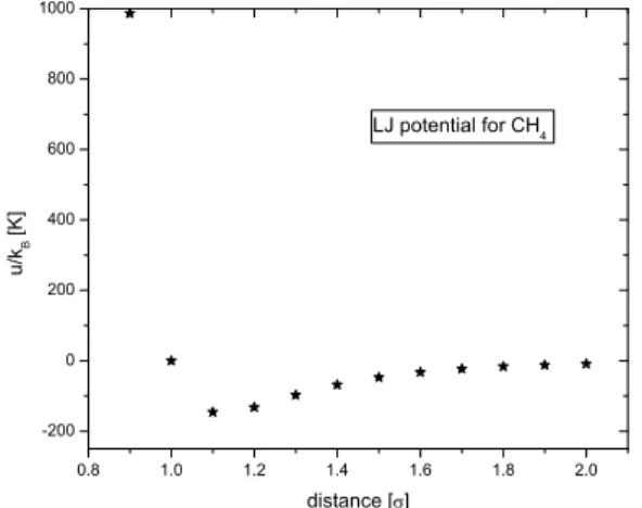
The symbolǫdenotes the depth of the potential well, whileσis the diameter of the molecular ”hard core”. Obviously, limr→0u(r) =∞. It can simply be shown that limr→σu(r) = 0 and that (∂u(r)/∂r) = 0 for
rmin = 21/6σ. The depth of the potential well is
u(rmin) =−ǫ.
An example of the LJ potential drawn for the particular case of CH4, with values ofǫ andσfrom (Reichl 1988), is represented in Fig. 1. This particu-lar molecule is interesting in two research fields: the planetary science, because it is present in the atmo-spheres of the giant planets, but also in studies of the interstellar medium. In the figure, the distance is expressed in units of σ and the potential divided by the Boltzmann constantkB given in units ofK.
0.8 1.0 1.2 1.4 1.6 1.8 2.0 -200
0 200 400 600 800 1000
u
/
k
B
[
K
]
distance []
LJ potential for CH 4
Fig. 1. The LJ potential for methane (CH4).
2. THE METHOD OF CALCULATION OF THE CHEMICAL POTENTIAL
Chemical potential of a fluid (or any other sys-tem) can be calculated in two different ways: by us-ing the general thermodynamical formalism, or by the general formalism of statistical mechanics.
2.1. The thermodynamical formalism
In this approach the calculation starts from the definition of the Gibbs potential:
G=U −T S+P V (2)
where all the symbols have their standard meanings. Using the virial expansion, the pressure can be ex-pressed as (Landau and Lifchitz 1976):
P∼=PID(1 +
N
V B) (3)
where N is the number of particles in the system and V the volume. The symbol B denotes the sec-ond virial coefficient, given by:
B= 1
2 Z ∞
0
(1−exp−u(r)/T
)dV (4)
andPIDis the pressure of the ideal gas. The symbol
u(r) denotes the interaction potential. Inserting Eq. (3) into Eq. (2), it follows that
G=U −T S+P V =GID+N PIDB . (5)
Chemical potential is defined as µ =
(∂G/∂N)P,T, which implies that:
µ= (∂GID
∂N )P,T+PIDB+N B(
∂PID
∂N )P,T (6)
or
µ=µID+PIDB+N B(∂PID
∂N )P,T. (7)
The equation of state of ideal gas is PIDV = N T
which finally leads to
µ=µID+ 2PIDB . (8)
For the particular case of the LJ potential, it can be shown that the second virial coefficient is given by (Reichl 1988):
B(T) =−(b0/2) ∞ X
n=0 1
n!Γ( 2n−1
4 )(
ǫ T)
2n+1 4 (9)
µ=µID−b0pID
∞ X
n=0 1
n!Γ( 2n−1
4 )(
ǫ T)
2n+1 4 (10)
which is the result for chemical potential. Limiting the sum in this expression to terms up to and includ-ingn= 1, it follows that:
µ∼=µID+ 2pIDb0 h
2.45083−1.8128(ǫ
T)
1/2i
×(ǫ
T)
1/4. (11)
2.2. The formalism of statistical mechanics The chemical potential of a fluid is given by (Hill 1987):
µ kBT
= ln(ρλ3) + ρ
kBT
Z 1 0 dγ Z ∞ 0 dr
×4πr2u(r)g(r) (12)
where γ denotes the ”coupling parameter” (Hill 1987), ρ is the particle number density , u(r) the interaction potential and g(r) is the radial distribu-tion funcdistribu-tion. The symbol ¯his the Planck constant divided by 2π, m is the particle mass and λ is the thermal wavelength given by
λ= ( 2π¯h 2
mkBT
)1/2.
Expression (10) is valid under the conditionρλ3>1, which leads to:
ρ≥
µ
mkBT
2π¯h2
¶3/2
. (13)
The radial distribution function is a ”bridge” relating macroscopic thermodynamic properties with interparticle interactions in any kind of a substance. In the theory of liquids,g(r) can be determined from first principles (Hill 1987) just by assuming a suit-able form of intermolecular potential (Morsali et al. 2005). In what follows, the result for g(r) obtained in Morsali et al. (2005) will be used. Changing the variable fromrtox=r/σ, and performing the inte-gration overγ, it follows that:
µ
kBT = ln(ρλ
3) + 4πσ3 ρ
kBT
Z ∞
0
dxx2u(x)g(x).
(14) The domain of integration can be divided into two subdomainsx∈[0,1] andx∈[1,∞]
I=σ3Z ∞
0
dxx2u(x)g(x) =
σ3[Z 1
0
dxx2u(x)g1(x) +Z ∞
1
dxx2u(x)×g2(x)]
=σ3×[I1+I2]. (15)
The divergence of the LJ potential which occurs whenx→0 can be bypassed either by introducing a suitable change of the range of integrationx∈[x0,1] instead ofx∈[0,1] withx06= 0, or by changing the form of the potential in the domainx ∈ [0,1]. For
x∈[0,1] the functiong(r) has the form
g1(x) =sexp[−(mx+n)4] (16)
and forx∈[1,∞] the radial distribution function is
g2(x) = 1 + 1
x2exp[−(ax+b)] sin[(cx+d)] + 1
x2exp[−(gx+h)] cos[(kx+l)] (17)
wherea,b,c,d,g,h,k,l,m,nandsare functions of pressure, temperature and density given in Morsali et al. (2005).
The appropriate boundary conditions, that the radial distribution function should tend to 1 in the limits of zero density and infinite distance, and the consequences of these conditions are also dis-cussed there. As a consequence, the functionsb,d,h
andl are functions of density only,nis the function of temperature only and the other functions depend on the temperature and density (Morsali et al. 2005).
3. THE CALCULATION
3.1. The case x∈[0,1]
With the change of variables x=r/σ, the LJ potential gets the form:
u(x) = 4ǫ[x−12 −x−6
]. (18)
Inserting Eqs. (16) and (18) into the expres-sion forI1 in Eq. (15), it follows that:
I1= 4sǫ ∞ X
l=0 (−1l)
(l!) Z 1
x=x0
( 1
x10 − 1
x4)
(mx+n)4ldx . (19)
Performing the integrations, after some alge-bra, it finally follows that:
I1∼= 8
9sǫ×[1 + 27
5 m 4−
27 10m
8−9m12 54 +..+
1 2x9
0 − n
4
2x9 0
3.2. The case x∈[1,∞]
In this case, the calculation of chemical po-tential is more straightforward. Inserting Eqs. (17) and (18) into the expression for I2 in Eq. (15), and performing the integration, gives the following ap-proximate result for the integral I2:
I2∼=−8ǫ
9 +πǫcos[d] cosh[b][
a5 120 −
a3c2 12
+ac 4
24 −
c
5cos[c] cos[d] +. . .]. (21)
3.3. The chemical potential
According to Eqs. (14) and (15) chemical po-tential is given by:
µ=kBTln(ρλ3) + 4πρσ3(I1+I2) (22) where the first terms ofI1 andI2 are given by Eqs. (20) and (21).
Inserting Eqs. (20) and (21) into Eq. (22), one gets a simple analytical approximation for chemical potential of a LJ fluid.
4. DISCUSSION AND CONCLUSIONS
In this paper, we have obtained an approxi-mate analytical expression for chemical potential of a Lennard Jones fluid. Two ways in which such an expression can be obtained have been presented, and both of these approaches have been applied.
The approach based on the general thermo-dynamic formalism gives a result, expressed as Eq. (10), which is both mathematically and physically simpler. It contains just two variables which char-acterize the material under consideration - these are
σ - the diameter of the molecular ”hard core”, and
ǫ - the depth of the potential well. Note that the chemical potential obtained in this way for a certain value of the ratio ǫ/T reduces to the valueµID.
The formalism of statistical mechanics is both mathematically and physically more complex. The general conclusion is that the chemical potential de-pends on thermodynamic parameters of the fluid through the functions a-s, which are in turn func-tions of the pressure and/or density and/or temper-ature (Morsali et al. 2005), but also on the inter-action parameters. The approximate expression for chemical potential of a LJ fluid is:
µ∼=kBTln(ρλ3) +32
9 πρǫσ
3s[1 +27m4 5
+..+ 1 2x9
0
+..+a 3
s cos[d] cosh[b](
3a2 320 −
3c2 32) +..]. (23)
All the symbols in this expression have their stan-dard meanings, or were introduced in Morsali et al. (2005). Mathematically, the symbol x0 denotes the cut off radius of the LJ potential introduced in cal-culations in order to avoid the occurence of diver-gences. Physically, this quantity represents the inter-particle distance at which the pressure ionisation oc-curs. Qualitatively speaking, the pressure excitation and/or ionisation occur because electronic energies change under the influence of the external pressure field. For details about this process see, for example, Kothari (1938).
The calculation presented in this paper was motivated by recent advances in planetary science. As a consequence of numerous discoveries of giant ex-oplanets, modellisation of their internal structure has regained importance. These planets consist mostly of fluids, and accordingly an obvious need for a the-oretical ”preparation of the ground” for the modelli-sation of their interiors has occured. Studies of phase equilibrium and phase transitions demand an explicit knowledge of chemical potential. Some preliminary results in that direction have recently been obtained (Celebonovic 2009) in the limit of small density and without taking into account chemical potential. An-other interesting problem, which becomes accessible for study with the results obtained in this paper is the behaviour of chemical potential of a LJ fluid with changes of its thermodynamical parameters. Some aspects of both of these problems will be discussed in a future work.
Acknowledgements– This work was financed by the Ministry of Science Technology and Development of Serbia under its project 141007. I am grateful to the referee for helpful comments about the previous version of the manuscript.
REFERENCES
Celebonovic, V.: 2009,Publ. Astron. Obs. Belgrade, 86, 319.
Dzyaloshinskii, I. E., Lifchitz, E. M. and Pitaevskii, L. P.: 1961, Sov. Physics-Uspekhi,4, 153. Hill, T. L.: 1987, Statistical Mechanics: Principles
and Selected Applications, Dover Publications Inc., New York.
Lai, X. Y. and Xu, R. X.: 2010, arXiv:1011.0526 v2. Landau, L. D. and Lifchitz, E. M.: 1976,
Statistich-eskaya Fizika, Nauka, Moscow.
Kothari, D. S.: 1938,Proc. Roy. Soc.,A165, 486. Margenau, H.: 1939,Rev. Mod. Phys.,11, 1. Morsali, A., Goharshadi, E. K., Ali Mansoori, G. and
Abbaspour, M.: 2005,Chemical Physics,310, 11.
HEMIJSKI POTENCIJAL LENARD-ONSOVOG FLUIDA
V. ˇCelebonovi´c
Institute of Physics, Pregrevica 118, 11080 Zemun-Belgrade, Serbia
E–mail: [email protected]
UDK 52–335 Prethodno saopxtenje
U ovom radu izveden je na dva naqina analitiqki izraz za hemijski potencijal Lenard-onsovog fluida. Izraqunavanje je
izvedeno koristei termodinamiqki
for-malizam, kao i formalizam statistiqke
mehanike. Oblast integracije je podeljena na dve pod-oblasti. Dobijeni rezultati bie korisni u svim istraжivanjima vezanim za ravnoteжu faza i fazne prelaze u