No 586 ISSN 0104-8910
Equity–Premium Puzzle: Evidence From
Brazilian Data
Rubens Penha Cysne
Equity-Premium Puzzle: Evidence From
Brazilian Data
Rubens Penha Cysne
yApril 9, 2005
Abstract
This paper uses 1992:1-2004:2 quarterly data and two di¤erent methods (approximation under lognormality and calibration) to eval-uate the existence of an equity-premium puzzle in Brazil. In contrast with some previous works in the Brazilian literature, I conclude that the model used by Mehra and Prescott (1985), either with additive or recursive preferences, is not able to satisfactorily rationalize the equity premium observed in the Brazilian data. The second contribu-tion of the paper is calling the attencontribu-tion to the fact that the utility function may not exist if the data (as it is the case with Brazilian time series) implies the existence of states in which high negative rates of consumption growth are attained with relatively high probability.
1
Introduction
It has been now twenty years since the seminal paper by Mehra and Prescott (1985) raised the question of the "Equity-Premium Puzzle".
This is the name economists give to the fact that basic representative-agent models of asset pricing (e.g., Lucas (1978), Breeden (1979) and Mehra and Prescott’s (1985) adaptation of Lucas’ (1978) work1) have not been able
I am thankful to the participants of workshops at the Graduate School of Economics of the Getulio Vargas Foundation for their comments. The usual disclaimer applies. Key-words: Equity Premium, Puzzle, Brazil, Recursive Preferences, Asset Pricing. JEL: G12, E40.
yProfessor of Economics at the Graduate School of Economics of the Getulio Vargas
Foundation (EPGE/FGV) and a Visiting Scholar at the Department of Economics of the University of Chicago. E-mail: [email protected].
1To be detailed later in this paper. These models are usually denominated CCAPM
to satisfactorily rationalize the fact that US real returns on stocks have been, between 1889 and 1978, about six percent per year higher than those on T-Bills.
The title Mehra and Prescott used in their (now) famous article generated a curious semantic herd behavior in the profession. What should be just one more case of the universal problem regarding the failure of a certain model to explain a certain data set was named a "puzzle". Following the trend, several other macroeconomically disappointing exercises of statistically unsatisfactory analysis2, pertaining to the domain of what is usually dubbed
"calibration", were also given the name "puzzle".
Among these is the "risk-free rate puzzle", introduced in the literature by Weil (1989). This puzzle relates to the (low) long-run level of Treasury returns in the United States, when compared to those implied by Mehra and Prescott’s - type models.
Consistently with the underlying time frame of their model, Mehra and Prescott used US long-term data. Here, because long-term data is not avail-able for Brazil, I follow Sampaio (2002), Bonomo and Domingues (2002), Alencar (2002) and Issler and Piqueira (2000, 2002) and use short-term data. Relatively to these previous works, this work uses data of a more recent pe-riod.
The economic reasoning behind the …rst two puzzles cited above is as follows. Assets paying higher returns should do it, in equilibrium, according to the basic asset-pricing models previously mentioned, based on the fact that they present a higher covariance with the consumption stream of the representative agent. However, the empirical data for the US has shown that, under the values of the risk-aversion and of the time-discount parame-ters which are considered to be reasonable, stock returns’s covariance with consumption is not su¢ciently greater than that of Treasury Bills, in order to explain the observed di¤erence in their yields. This is what is behind the "equity-premium puzzle".
To explain the high spread between stocks and bonds, one needs values of the risk-aversion parameter that are considered too high. Assuming standard utility functions, in which the risk aversion equals the inverse of the elasticity of substitution, this is to say that agents should highly dislike growth. How-ever, if this were true, the necessary risk-free rates to explain the amount of saving in the US, an economy in which real per-capita consumption growth reaches almost two percent per year, should be much higher than the histori-cal one percent per year observed in the data. This leads to Weil’s "risk-free
2See, e.g., Browning, Hansen and Heckman (1999). Of course, the criticism extends to
rate puzzle" to which I have referred above.
Such puzzles emerge under the assumptions of complete markets, costless asset trading, and that consumer preferences can be represented by the stan-dard utility function used in macroeconomics. Explanations of the puzzles, therefore, can always be made by leaving aside one or more of these three assumptions. There must be, though, consistent support from the empirical evidence in doing so3.
A considerable amount of academic research has been developed attempt-ing to solve these puzzles. The explanations include simply denyattempt-ing the existence of a puzzle (see, e.g., Cecchetti and Mark (1990)), or arguments based on: i) recursive utility (Epstein and Zin (1991)); ii) habit formation (e.g., Constantinides (1990), Campbell and Cochrane (1999); iii) idiosyn-cratic risk ((Heaton and Lucas 1996, Constantinides and Du¢e (1996)); iv) probability of a large drop in consumption (Rietz (1988)); v) borrowing con-straints (Davis and Willen (2000)); vi) liquidity premium (Bansal and Cole-man (1996)) and; vii) changes in tax rates (McGrattan and Prescott (2001)). In the present work, the only departure from the assumptions outlined in Mehra and Prescott (1985) that I shall consider regards the modi…cation of the utility function to allow for Kreps-Porteus (1978) preferences, in the line of Epstein and Zin (1991).
In Brazil, some papers concerning, among other subjects, the possible existence of these two puzzles, have been conveniently collected in a book edited by Bonomo (2002). In the second part of this book, three di¤er-ent techniques have been used by several authors in order to assess if the CCAPM models could explain the respective data generated by the Brazil-ian economy. Among these, Sampaio (2002) follows the basic methodology used by Mehra and Prescott. Bonomo and Domingues (2002) innovate by modeling the consumption series using a Markov-switching model and also by using a Kreps-Porteus (1978) utility function. Alencar (2002) uses the approach of Hansen and Jagannathan (1991), interpreting the equity pre-mium puzzle in terms of the "market price of risk" generated by the data, and constructing volatility bounds. Finally, Issler and Piqueira (2000 and 2002), approach the problem by testing the Euler equations implied by three di¤erent models.
A common fact about these works is that they …nd either that "there is no equity-premium puzzle in Brazil (Issler and Piqueira (2000, p. 233),
3For instance, one could abandon the hypothesis of costless trading and argue that the
Bonomo and Domingues (2002, p. 116) and Sampaio4 (2002, p. 99) or that
there is a puzzle, but it less intense than the one which emerges with data related to the US (Alencar, p. 152)5.
When one concentrates solely on the basic assumptions of the model underlying these empirical analyses, such a conclusion of nonexistence of an equity-premium puzzle is intriguing. Indeed, it is hard to argue that Brazil would be any closer to complete markets or costless stock trading than the United States, United Kingdom, Japan, Germany, and France, just to cite some countries where the empirical failure of CCAPM models has been documented6 (see, e.g., Allais and Nalpas (1999), Iwata (1996), Canova
and Nicolo (1995) or Mehra (2003)).
Under this view, the purpose of the present work is reassessing if the Mehra and Prescott’s model, either under the usual CRRA utility or under recursive utility, can be indeed a reasonable model to explain the returns on equities and risk-free bonds in Brazil.
My conclusions here are contrasting with those obtained by Sampaio (2002), Bonomo and Dominges (2002) and Issler and Piqueira (2000, 2002). I have not been able to explain the Brazilian equity-premium with Mehra and Prescott’s model. On the other hand, I have found no evidence of "an inverted risk-free puzzle", as pointed out by Bonomo and Domingues (2002). The model is able to satisfactorily explain the risk-free rates of interest pre-vailing in Brazil. Such a contrast in the conclusions can be found in many di¤erent grounds, including di¤erent data sets, distinct methodologies, and the use of alternative discrete-state modelings of the consumption-growth series.
The remaining of this work proceeds as follows. Sections 2 and 3 present the basic model and the conditions for the existence of an expected utility. Section 4 is used to discuss the new data set from which I derive new re-sults, and to compare it with the data sets used by other authors. Section 5 displays new empirical outcomes, initially in the form of approximations under assumptions of lognormality and, next, as the asset returns implied by the simulations. Given the contrasting evidence regarding the empirical results of this work and of its predecessors, Section 6 o¤ers tentative expla-nations for such discrepancies. Section 7 recalculates the simulations under
4In the case on non-seasonally adjusted data.
5Soriano, though, arrives at this milder conclusion by considering seasonally adjusted
data. The remaining works, including the results I report here, were based in nonseasonally adjusted data.
6As pointed out by Mehra (2003), the United States, the United Kingdom, Japan,
the assumption of recursive utility. Section 8 concludes.
2
The Basic Model
Mehra and Prescott (1985) have adapted Lucas’s (1978) pure-exchange model by assuming that consumption growth, rather than consumption itself, fol-lows a …rst-order Markov process. This adaptation aims at capturing possible nostationarities of the real per-capital consumption series.
I describe the model below using initially an Arrow-Debreu structure with contingent claims all traded at time 0. Next, I assume a Markovian structure of endowments and use the pricing sequence previously obtained to price one-period Arrow securities in a sequential-trading structure.
There are several identical consumers in the economy. A representative consumer maximizes the discounted utility (U) of consumption (c)7:
U(c) =E0 1
X
t=0
t
u(ct); 0< <1 (1)
or, given the assumption of a …nite number of states, and with t standing
for the history of states till time t :
U(c) =
1 X t=0 X t t
u(ct( t)) 0t( t)
subject to the constraint:
1
X
t=0 X
t qt0(
t
)ct( t)
1
X
t=0 X
t qt0(
t
)et( t) (2)
Above, stands for the time-discount parameter, Et for the expectation
conditional on the information available at time t; q0
t for the time-zero price
of a security promising to pay one unit of consumption at time t; 0
t for the
conditional probability (on the information available at time zero) of having
the history t and
et for the endowment at time t: Equation 2 uses the fact that the linear functional de…ned in the commodity space of the problem has a dot product representation8.
7By assumption lim
c!0u(c) =1and u(c) is concave.
8Note that with exogenous growth the commodity space cannot be the usual l
1:
Make 1 +gt+1 = etet+1, the aggregate endowment growth in period t+ 1.
Endowments are assumed to be governed by a Markov process. In equi-librium, endowments will also be equal to the real per-capita consumption growth.
Assume that:
u(c) = c
1 1
1 ; 0< <1 (3)
In the present description of the model, at time t0 households trade claims
on the time t consumption good at all nodes t: After t0; no further trade
occurs. There are no enforcement- or information-related incentive problems. The equilibrium allocations in this economy are equivalent to those of an economy with sequential trading. In particular, the allocations at each point in time depend only on the realized aggregate endowment. It is also assumed that the necessary and su¢cient condition for the existence of the utility function given by Proposition 1 below is satis…ed.
Under such circumstances, the price/dividend ratio Q can be easily de-termined, after a straightforward application of the Kuhn-Tucker theorem (the point of departure of which, in this in…nite-dimensional case, is the Hahn-Banach separation theorem).
First, use the auxiliary Lagrangean function to obtain:
qtt+1( t) =
u0
(ct+1( t+1))
u0
(ct( t)) t+1(
t+1
j t) (4)
This expression gives the time-t price of an asset that pays o¤ 1 if history
t+1 comes true, given that t has happened.
Next, (4) will be used to price an ex-dividend one-period ahead stock, at time t:
Because of the Markovian structure that we assume for the endowment process, decisions taken at date t only depend on the state variables at this date, and not on the whole history till date t ( t). This allows us to work
conditionally only on the information set available at time t, and only
con-sider the possible states that can be reached at datet+ 1, instead of having to keep track of all previous history t
;as in (4).
sequences of vectors with the t th vector indexed by the eventet= (g1; g2; :::; gt):The
set of possible period t events is called Et;and has cardinalityn t
:The norm of an element z2L is given by:
kzk= sup
t
max
et2Et j zt(et)
yt
j
Call the sequential-trading price of an ex-dividend one-period ahead stock
Qt. Then. using (4):
Qt( t) =
X
t+1
u0
(ct+1( t+1))
u0(ct(
t))
(Qt+1( t+1) +et+1( t+1)) t+1( t+1 j t) (5)
Dividing both terms byet+1and using (3) leads to the following expression
for the price/dividend relation Pt=Qt=et:
Pt=X
t+1
((1 +gt+1( t+1))1 ) t+1( t+1 j t)(Pt+1( t+1) + 1) (6)
The expected equity return conditional on the information available in time
t is given by:
1 +rt+1= X
t+1
Qt+1( t+1) +et+1( t+1)
Qt t+1( t+1j t)
Making
Qt+1+et+1
Qt =
et+1
Qt (1 + Qt+1
et+1
)
one gets, after multiplying and dividing the above expression byet:
1 +rt+1 = X
t+1
(1 +gt+1( t+1)) t+1( t+1 j t)
1 +Pt+1( t+1)
Pt (7)
To obtain the risk-free rate note that (5) allows us to write, for m = r or m =rf (rf standing for the risk-free rate):
1 =X
t+1
u0
(ct+1( t+1))
u0(ct) (1 +mt+1) t+1( t+1 j t) (8)
From which we get (also conditional on the information set available at time
t; and noticing that by de…nition rft does not depend on the realization of t+1):
1 +rft+1 =
1
X
t+1
(1 +gt+1( t+1)) t+1( t+1 j t)
3
Existence of the Expected Utility
As pointed out by Mehra and Prescott (1985, p. 151), the introduction of nonstationarity in Lucas’s (1978) model requires, among other things, veri-fying if the conditions under which the expected utility exists are satis…ed. The Proposition below, the proof of which Mehra and Prescott (1985, p. 151) refer the reader to Mehra and Prescott (1984), provides a direct way to check it.
Proposition 1 (Mehra and Prescott (1984)): Suppose the preferences of the representative consumer are ordered over random paths by (1) and (3). Denote by W the transition matrix of the (ergodic) Markov chain associated withgt+1 2 fg1; g2; ...,gNg,gi 0 for alliand alltand suppose thate0 >0: Then, a necessary and su¢cient condition for expected utility to exist is that the matrix A with elements ai;j = Wi;j(1 +gj)1 obeys:
limm!1Am = 0 (10)
Proof. See Mehra and Prescott (1984) or Mehra (1988).
Note that the condition (10) is equivalent to the matrixA having eigen-values all of which lie within the unit circle in the complex plan.
An intuition of this result is easily obtained from the analysis of the deterministic case, in which, trivially,EU(c)<1if and only if (1+g)1 <
1: In the stochastic case, one has to consider all states attained by g. In
particular, note that when is very high (in an attempt of the researcher to obtain high equity premia with the model) one can easily have (1+g)1 >1
for values ofgslightly below zero. This can pose a problem for the ful…llment
of condition (10).
Condition (10) is also su¢cient to guarantee a unique positive solution tot thenbynsystem of linear equations (when n states are considered) given
by (6).
4
Data
Population data are from the FIBGE. For the two …rst quarters of 1994 population data were extrapolated under the assumption that the rate for 2004 was the same as the one for 2003. Within each year the series was quarterly interpolated assuming a log-linear growth.
The price index used to de‡ate consumption and to obtain real interest rates was the INPC (Índice Nacional de Preços ao Consumidor) provided by the FIBGE. The Selic (Sistema Especial de Liquidação e Custódia) in-terbank rate was used to generate the "risk-free" rate, and the return of the IBOVESPA index to generate the equity rate (a claim to the stochastic endowment). Both were de‡ated by the in‡ation rate calculated using the INPC. The source of the Selic and of the FGV-100 was the databank of the IBRE (Instituto Brasileiro de Economia da Fundação Getulio Vargas).
Table 1 summarizes the data used by di¤erent authors, including Prescott and Mehra for the US and Sampaio (2002), Domingues and Rodrigues (2002), Issler and Piqueira (2000, 2002), Alencar (2002) and Cysne (this work) for Brazil.
Table 1 - Data (%) on Per.Cap. Cons. Growth (g) and Real Returns
Range/Per. av(g) st(g) av(r) st(r) av(rf) st(rf) e.p.
M./P. (US) 1889-78 A 1.83 3.57 6.98 16.54 0.80 5.67 6.18 Sampaio 1980-98 Q 2.02 7.20 29.13 29.30 7.82 9.70 21.31
B./D. 1986-98 Q 0.80 6.80 24.21 31.12 13.96 6.28 10.25 I./P. 1975-94 A - - - 29.06 Alencar 1980-98 Q 1.61 2.2 28.65 29.1 7.40 5.70 21.25 Cysne 1992-04 Q 3.12 4.80 31.33 24.89 15.41 4.82 15.92
av=average, st=st. dev., r = equity rate, rf = risk-free rate, e.p.=equity premium
Q=Quarterly, A=annual, Per=Periodicity, M./P = Mehra and Prescott (Table 1, p. 147) B./D. = Bonomo and Domingues (Tables 1 and 2, p. 106)
I./P. = Issler and Piqueira (p. 234 of I./P. (2000)). Data for Alencar comes from Table 2, p. 128 and for Sampaio from Table 1, p.194.
calculate the mean return on equities using the IBOVESPA (Índice da Bolsa de Valores do Estado de São Paulo).
In Table 1, concerning the brazilian economy, this work (last row in Table 1) presents the highest value of the per capita consumption growth. This is consistent with the fact that after the Real Plan there were high current account de…cits, fostering consumption temporarily. The standard deviation of 0:048 (of consumption growth) is higher than the one reported by Mehra
and Prescott (1982) for the US time series (0:036): But lower than the ones reported by Sampaio (0:072) and by Bonomo and Domingues (0:068), for
Brazil. This re‡ects the fact that these previous studies using Brazilian data included a larger share of the period in which in‡ation was higher. Relatively to the data I present here, they do not include the 1998-2004 low-in‡ation period.
This work also presents the highest risk-free rate(15:41%);a consequence of the fact that after the Real Plan high interest rates were used to control the residual in‡ationary pressures. Last, note that the equity premium calcu-lated here (15:92%) is between the one calculated by Bonomo and Domingues (10:25%) and those calculated by Issler and Piqueira (29:06%) and by
Sam-paio (21:31%).
Figure 1 below presents the data in a way close to the one Mehra and Prescott (1985, Table 1) and Kocherlakota (1996, Table 1) did in their re-spective works:
Insert Figure 1 Here
The numbers in the …rst column of Figure 1 correspond to the averages presented in the last row of Table 1. However, in Table 1 they are expressed in an annual and percentage basis, whereas Figure 1 presents them in a quarterly and decimal basis. The quarterly standard deviations reported in the last row of Table 1 can also be obtained from Figure 1.
Note that, as it happens with the data reported in Mehra and Prescott (1985), the sample covariance of consumption growth and the return on eq-uity (0:00208) is higher than the sample covariance on consumption growth and the return on the risk-free asset ( 0:00032)9. This implies that the
model we have seen in the last section does account for the fact that the return on equity (which pays more when consumption is higher) is observed to command a certain premium over the return on the risk-free rate. We shall see, though, that although qualitatively right, the CCAPM model is not able to provide a satisfactory quantitative rationalization for the equity premium found in the Brazilian data.
5
Empirical Results
5.1
Preliminary Analysis Under Lognormality
Before calibrating a general-equilibrium model as in Mehra and Prescott (1985), I investigate the existence an equity premium puzzle assuming log-normality of returns.
The expressions for asset returns under lognormality are well known in the literature (see, e.g. Hansen and Singleton (1983) or Ljungqvist and Sargent (2002)), being included here just for completeness.
Suppose that consumption growth, the equity return (r) and the risk-free return follow the equations:
1 +kt+1 = (1 +k) exp("k;t+1 2k=2); for k =g; k = r ork =rf (11)
with {"g;t+1; "r;t+1; "rf;t+1} jointly normally distributed with zero means and
variances { 2
c; 2r; 2rf}. By using the fact that the moment generating
func-tion of a standard normal variable (E(exp( Z)) is equal to exp( 2=2); one
easily concludes that the expected value of1 +kt+1 in (11) isk. This allows
for an economic interpretation of (11) that is used below.
From equations (5) and (3), applying the law of iterated expectations:
1 = E (1 +gt+1) (1 +mt+1) ; for m=r orm =rf (12)
Using (11) in (12), form=r or m=rf:
1 = (1 +g) (1 +m) E exp ("m;t+1 2m=2) ("g;t+1
2
g=2) (13)
Since the variable between brackets is a normal variable with mean 2
m=2 +
2
g=2 and variance 2m+ 2 2g+ 2 cov("m; "g);using again the result above
for the moment generating function of a standard normal variable (form=r
or m=rf):
1 = (1 +g) (1 +m) exp((1 + ) 2g=2 cov("g; "m)) (14) Taking logarithms on both members of (14):
log(1 +m) = log + log(1 +g) (1 )
2
g
2 cov("g; "m) (15)
Making for m = r and m = rf above and and subtracting the resulting
expressions:
Since log(1 +x) ' x for low (absolute) values of x; (16) allows us to use
the sample values of cov("g; r); cov("g; rf); and the means of r and rf; in
order to obtain the implied risk-aversion parameter . Approximating these covariances with the values of Figure1, we get = 14:15;or directly from the
values of Figure 2, = 15:8: One can also use the fact that the populational value of cov("g; rf) is equal to zero, to obtain even higher values fo (16:36
and 19:12, respectively): In any case, it is clear form the data the existence
of an equity-premium puzzle (since >10is not acceptable as a reasonable range for the parameter ).
Insert Figure 2 Here
5.2
Existence and Calibration
Since the calculations above relied on the assumption of lognormality, the conclusions may have resulted from this hypothesis, rather than from the empirical failure of the underlying model. In this subsection I abandon the hypothesis of lognormality and re-investigate the existence of an equity-premium puzzle under another set of assumptions.
I assume that real per-capita consumption growth (g) follows a linear
stochastic di¤erence equation driven by a Gaussian disturbance, and that it can be reasonably modeled by a stationary AR(1) process:
gt=bgt 1 +"t (17)
where " is a normal random variable with mean a.
Using (17) and the value of b estimated from the sample data, one
con-cludes that "t has an average equal to 1:0016 and a standard deviation of 0:0480:Based on these data, I generate an approximation of the initial prob-lem using ten di¤erent states for g and a transition matrix T of the
approx-imating discrete-state Markov chain.
The minimum and maximum values of the series of consumption growth are 0.9065 and 1.1016, respectively In the discrete-state approximation, such values are, respectively,0:91and1:1010. The states and the stationary
prob-abilities are presented in Figure 3.
Insert Figure 3 Here
10The Markov chain implied by the data and its discrete-state approximation have also
Checking the Existence of an Expected Utility
Before starting the simulations, it is crucial to check if, under the pa-rameter values used in the problem, the necessary and su¢cient conditions for the existence of an expected utility function are satis…ed. This is done with the help of Proposition 1. The calculations using beta, the transition matrix and the ten states of consumption growth show that Proposition 1is satis…ed for the values of the gammas used in the simulations (from 2 to 6) but not necessarily for >7 (when = 0.995) or >9 (when = 0:9740).
The fact that the series of real per capita consumption growth used here has a higher average and a lower standard deviation than the ones used by Sampaio (2002) and by Bonomo and Domingues (2002) plays an important role in the existence of the expected utility (an inspection of condition (10) makes this point clear).
Calibration
The calibration I carry out in this section has the advantage, when com-pared with those reported by Sampaio, and by Bonomo and Domingues, of approximating the consumption series with ten states, instead of only two.
The equity premium implied by the model is generated in the following way. First, the continuous state Markov chain is approximated by a ten-state Markov chain, as detailed above. Second, the transition matrix is used to simulate a time series of length 15000 for the states assumed by the Markov chain. Third, for each state, di¤erent values of the parameters ( ; )and (6)
are used to calculate the price/dividend ratios. Fourth, such price-dividend ratios are used to calculate, also for each state, the return on equity, the risk-free rate and the equity premium. In this step I used (7), (9), and the fact that the equity premium is de…ned as r rf: Fifth, the 15000 states
assumed by the Markov chain are employed to generate time series of r, rf
and the equity premium. Sixth, I take the averages of each one of these series to obtain the equity return, the risk free rate and the equity premium generated by the model11.
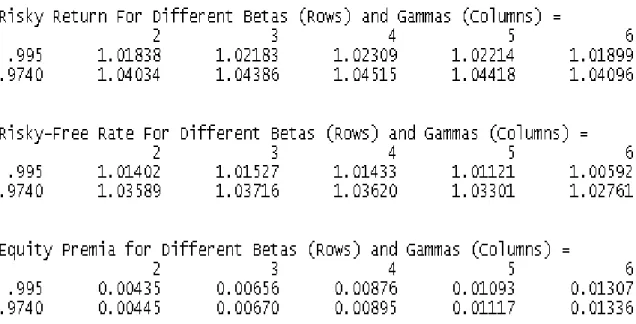
The results of these steps are presented in Figure 4.
11Since the Markov chain under consideration is ergodic, the state space is compact and
the transition function de…ned by annbynstochastic matrix de…nes a stable conditional
Insert Figure 4 Here
Note in Figure 4 that both the equity return and the risky-free rate de-crease for high values of gamma. Under deterministic growth, interest rates vary positively with the risk aversion parameter when consumption-growth rates are strictly positive (equation (15) withm=rf makes this point clear).
When the variance of consumption growth is not zero, though, this rate tends to become a negative function of when this parameter assumes higher val-ues (see equation (15) once more): As one can observe from Figure 3, states
1 to 5 considered in the simulations are characterized by negative rates of growth of consumption. Moreover, 2
g > 0 here. For these reasons, one can
get risk-free rates decreasing with the value of gamma.
From Table 1 or from Figure 1, the quarterly equity return for the 1992:01-2004:2 period should run around 7:052%, and the risk-free return around 3:648%, generating a quarterly equity premium around 3:40%. From Figure
4, the maximum equity premium generated by the model happens for = 0:974 and = 6;and is equal to1:34%. This result con…rms the preliminary
calculations carried out under the assumption of lognormality, concluding that there is an equity-premium puzzle in Brazil.
In section 7 I check if this puzzle remains under more elaborate utility functions.
When = 0:974, the quarterly risk-free rate which emerges from the sample is generated for values of the relative risk-aversion parameter between two and four. Since these are considered to be reasonable parameters for ;
I …nd no risk-free-rate puzzle as the one identi…ed by Weil (1989) for the United States. Neither an "inverted risk-free rate puzzle", as pointed out by Bonomo and Domingues (2002).
6
Comments on Previous Works
In section 5 I have found evidence of the existence of an equity-premium puzzle in the Brazilian data, both under a lognormal approximation and in the calibration exercise using Brazilian 1992:1-2004:2 quarterly data.
In contrast with this result, Sampaio (2002, p. 99), using nonseasonally adjusted quarterly data ranging from 1980:1 to 1998:2, …nds that the …rst mo-ments of Brazilian data can be obtained using Mehra and Prescott’s model for values of the risk aversion parameter ( )and of the time-discount parameter ( )equal to, respectively,6:1and0:91(quarterly):Sampaio (2002) concludes
Also in contrast with the results obtained here, Bonomo (2002, p. 116) states that "there is no equity premium puzzle in Brazil", whereas Issler and Piqueira (2000) argue that "there is no equity premium puzzle for Brazil due to the great variation observed for the equity premium" (page 233)12.
In the next paragraphs I analyze some of these works in order to under-stand the di¤erence in the conclusions.
Sampaio (2002) and of Bonomo and Rodrigues (2002):
A …rst point to note is that the data set used here di¤ers from the data set used in these works. Not only are the time periods di¤erent, but also the consumption series. I use o¢cial quarterly IPEA/FIBGE/Macrodados’s consumption data, including non-durables and durables, whereas Soriano, Sampaio (2002) and Bonomo and Rodrigues (2002) (see page 81 in Bonomo (2002)) use a private consumption series produced by Soriano, which excludes durables).
Below I use the data sets provided by Sampaio (2002) and by Bonomo and Domingues (2002) to show that the results reported by these authors do not survive under the lognormal approximation.
Second, also using the data reported by these authors, I show that, under the Mehra and Prescott’s methodology, the maximum possible range between states of consumption growth that these works could use falls short of the range displayed in their data. This is a condition implied by (10), on the existence of the expected utility.
Redoing the Calculations Under Lognormality
In order to redo the approximate calculations under lognormality, one needs the equity premia, as well as the covariance between consumption growth and the returns on equities and on the risk-free asset. Such data are not directly available, since Sampaio (2002) and Bonomo and Rodrigues (2002) do not report the sample covariances.
However, since these authors use the same real consumption series as Alencar (see Bonomo (2002), p. 81), and since the series of nominal returns are the same (IBOVESPA and Selic), I use the Table of variance/covariance for nonseasonally adjusted data published in Alencar (2002, p. 157. Table 9).
From this table, the di¤erence between the covariance of consumption and the risky rate, and the covariance of consumption and the nonrisky rate, using quarterly data, is equal to 0:00004. Sampaio (2002, p. 96. Table 2)
12Alencar (2002) cannot be used as a direct source for comparison, since this author
reports a quarterly premium of0:047whereas Bonomo and Domingues (2002,
p. 106, Table 1) report0:02247. Using (16), such values imply a risk-aversion parameter ( ) equal to, respectively, 1175:0 (!) and 561:75 13. In contrast
with the results obtained by these authors, this implies again, as I have found in this work, that there is an equity-premium puzzle in Brazil14.
Maximum Allowable Range Between States Implied by the Ex-istence of the Expected Utility
Neither Sampaio nor Bonomo and Rodrigues report for which range of the parameter values they use one could assure the existence of the expected utility function.
This condition is particularly important in the Brazilian case, because of the relatively lower average15 and higher standard deviation16 of the real
per-capita consumption growth (when compared to the US). These facts imply assigning relatively high probabilities to states in which real per-capita consumption decreases sharply, with (1 +g)1 assuming values that can
be too high for the expected utility to exist.
Sampaio (2002)
Using the parameter values and the number of states (equal to 2) re-ported by Sampaio (2002) I carry out next some calculations with this pur-pose. Using the parameter values of Table 1 in Sampaio (2002, p. 94) of
average consumption growth equal to0:005;standard deviation of consump-tion growth 0:072 and …rst-order autocorrelation 0:128, a implied2 state
Markov chain can be very conservatively (concerning the validity of Propo-sition 1)17 approximated with the states, stationary probabilities and
Tran-sition Matrix given by Figure 5.
13Using a covariance with the risk-free return equal to zero does not improve the results
signi…cantly. The new numbers for gamma are now671:4 and321:0;respectively.
14One could argue that the approximation under lognormality would not be appropriate,
but this reasoning would not explain such high values of the risk-aversion parameter.
15Except in Sampaio (2002).
16The data reported by Alencar (2002) cannot serve as a basis of comparison here
because this author uses seasonally adjusted data.
17The states that emerge from the matrix of Figure 5, after the due adjustment in the
Please Insert Figure 5 Here
Note in Figure 5 that the two states of the approximation of the rate of growth of the endowments, 0:88260 and 1:12740; both lie within the range displayed in Figure 1 of Sampaio (2002, p. 94) (bye the eye, the sample range in Figure 1 of Sampaio (2002) goes from 0:85to 1:15): Moreover, the
weighed mean of the approximating states, using the stationary probabilities, exactly coincides with 1:005; the sample value of the average rate of growth of consumption reported by this author.
Increasing the range of the approximation would be supported by the data but would make things worse in terms of the existence of an expected utility. The number used here, therefore, are conservative.
Figure 5 also shows the values of the matrix A in Proposition 1, for = 6:1and = 0:91;which are found by Sampaio as those for which there is no premium puzzle. The maximum absolute value of the eigenvalues of this matrix is equal to 1:0547, implying that condition (10) is not satis…ed.
An alternative calculation, probably closer to the way how this author may have worked, is inverting the procedure and obtaining the maximum possible range for the rates of consumption growth that still allow for the existence of an expected utility. The results are presented in Figure 6. The new lower and upper bounds for the rate of consumption growth, respectively,
0:906and1:104;are farther away from the respective end points of the sample
values displayed in Figure 1 in Sampaio (2002).
Please Insert Figure 6 Here
Bonomo and Domingues
Bonomo and Rodrigues (2002, p. 111) argue that they have been able to reproduce the equity premium modelling consumption with Markov switch-ing usswitch-ing with a value of the parameters of time discount equal to 0:95 per
quarter and a value of the risk aversion parameter of 3:23.
Here I use the same data but model consumption growth di¤erently from these authors, using the procedure described in section 5 (though with only two states, as Bonomo and Domingues (2002) did), and check if their results would be robust under this alternative modeling18.
18Bonomo and Domingues approximate the logarithm of the consumption growth series
(log(1 +g)) using a Markov-switching model, rather than a discrete-state Markov chain of the relative change (1 +g), as I do here. For this reason, the evaluation of the existence
The values of the real per-capita consumption series are displayed in Table
2 of Bonomo and Rodrigues (2002, p. 106). The average and standard deviation of the real per capita consumption growth are equal to 0:002 and 0:068, respectively. The …rst order correlation coe¢cient is 0:075:
One can easily see from Figure1in Bonomo and Rodrigues (2002, p. 111) that 1:11is not a upper bound and 0:89 is not a lower bound ofg =ct+1=ct.
Acting conservatively, in terms of Proposition 1 (see footnote 17), in a next step I construct states, a transition matrix and stationary probabilities using the same procedure as I did in the case of Sampaio (2002), above. The result is displayed in Figure 7.
Please Insert Figure 7 Here
Note that the mean of the states is exactly1:002, as reported by Bonomo,
for the variable g. As it happened with the data of Sampaio, the maximum absolute value of the eigenvalues of the matrix of Proposition 1 is 1:0974, showing that for such an amplitude between states the expected utility does not exist.
As above, a more interesting calculation, using the data reported by Bonomo and Domingues, would be obtaining the maximum allowable range for the rates of consumption growth that would allow the existence of an expected utility. The results of such a calculation are shown in Figure 8.
Please Insert Figure 8 Here
The new lower and upper bounds for the rate of consumption growth
(1 + g), respectively, of 0:936 and 1:068; are now farther away from the
extremes of the sample values displayed in Figure 1 in Bonomo and Rodrigues (2002, p. 111)19.
Issler and Piqueira (2000, 2002)
The main purpose of Issler and Piqueira (2000, 2002) is not discussing the equity-premium puzzle (which is done only in the last pages), but to estimate structural parameters for the Brazilian economy for di¤erent types of utility functions. In the spirit of Hansen and Singleton (1982), these authors have tested a set of necessary conditions implied by the basic model and have not
19Both in Sampaio (2002) and in Bonomo and Domingues (2002), satisfying Proposition
been able to reject it, thereby their conclusion about the inexistence of an equity premium puzzle in Brazil.
The best way to contrast the evidence provided by Issler and Piqueira with the results found here would be through an empirical re-evaluation of the restrictions implied by the basic CCAPM model using the same data set I used here and the same methodology used by these authors. This is a good suggestion for future research in the area.
7
Empirical Results With Recursive Utility
A restriction imposed by the class of preferences we have used so far is that the same parameter ( )assumes simultaneously the role of the coe¢cient of risk aversion and of the reciprocal of the elasticity of intertemporal substi-tution. This implies that aversion to uncertainty among states of nature is necessarily related to aversion to consumption variation over time. Epstein and Zin (1991) use Kreps-Porteus (1978) preferences, a class of preferences that avoids this problem. Their recursive utility can be stated as:
Vt= ((1 )c1t + ( tVt+1)1 ) 1
1 ; 6= 1; 0< <1
where:
tVt+1 =Et(Vt1+1 ) 1 1
Proceeding as before, the expected price/equity ratio is now given by:
Pe
t =Et( ( ct+1
ct )
1 ( Vt+1
tVt+1
) (1 +Pe t+1))
Making Wt =Vt=et one has:
Pt=Et( (gt+1)1 (
gt+1Wt+1
t(gt+1Wt+1)
) (1 +Pte+1))
Note that this formula is equivalent to (6), except for the presence of the term
( gt+1Wt+1
t(gt+1Wt+1)) on the right member and for the fact that is replacing
and is replacing : The risk-free rate now reads:
rft = 1
Et( (gt+1) ( tgt(gt+1+1WtWt+1+1)) )
is now given by ; thereby being completely independent of the elasticity
of substitution 1= : =(1 ) can be interpreted as the new time-discount parameter (the beta of the previous section).
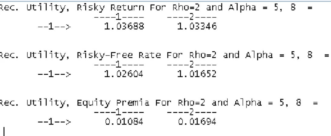
I redo the previous calculations for = 2 and = 5;6; in order to
compare with the previous case. The results are shown in Figure 9.
Please Insert Figure 9 Here
As it is clear from the last row of Figure 9, using recursive utility does not modify the fact that Mehra and Prescott’s-like models are not able to satisfactorily rationalize the equity premium found in the Brazilian data. On the other hand, the risk-free rate that is generated by the model with = 2
and = 5 is basically the same as the one observed in the sample. Again,
there is no risk-free rate puzzle, as the one reported by Weil (1989) for the U.S., or "inverted risk-free rate puzzle", as the one reported by Bonomo and Domingues (2202) for Brazil.
8
Conclusions
In this paper I have used 1992:1-2004:2 Brazilian quarterly data to evaluate the existence of an equity-premium puzzle. In contrast with some previous works in the Brazilian literature, I have concluded that the model used by Mehra and Prescott (1985), either with additive or recursive preferences, is not able to satisfactorily rationalize the equity premium observed in the Brazilian data.
Such a conclusion was obtained both under assumptions of lognormality or under simulations based on a discrete state approximation of the Markov process implied by the data. The model is able, though, to produce risk-free interest rates in agreement with those observed in Brazil.
An advantage of the modeling of consumption growth I have performed here over those of Sampaio (2002) and of Bonomo and Domingues (2002) is that I have used ten states, instead of just two.
I have also derived the maximum allowable range between states that these authors could use to model consumption growth under the Mehra and Prescott methodology. The results have shown a range very inferior to the one displayed by their data.
This last conclusion points out that the utility function may not exist (under the Mehra and Prescott methodolology) when one uses a small num-ber of states to approximate a consumption-growth series with relatively high standard deviation (as it happens with Brazilian data) and tries to rational-ize the equity-premium puzzle using values of the risk-aversion parameter that lie within the usually allowable range (0 to 10), but are otherwise too
high.
Finally, I have redone the calibrations using Kreps-Porteus (1978) prefer-ences and have maintained my previous conclusion that the usual CCAPM models cannot satisfactorily rationalize the equity premium implicit in the Brazilian data, even though they are able to generate the risk-free interest rates found in Brazil .
References
[1] Alencar, A. S. 2002. "Testando CCAPM Através das Fronteiras de Volatilidade e da Equação de Euler", in Bonomo, M., (Editor), "Fi-nanças Aplicadas ao Brasil", Editora da Fundação Getulio Vargas, Rio de Janeiro, p. 119-161.
[2] Allais O. and Nalpas, N. 1999. "The Equity Premium Puzzle: an Eval-uation of the French Case", mimeo, University of Paris I.
[3] Bansal, R., and J.W. Coleman. 1996. “A Monetary Explanation of the Equity Premium, Term Premium, and Risk-Free Rate Puzzles.” Journal of Political Economy, vol. 104, no. 6 (December):1135–71.
[4] Bonomo, M. A. 2002, Editor. "Finanças Aplicadas ao Brasil" ed. Rio de Janeiro : Fundação Getulio Vargas.
[5] Bonomo, M. A. C. and Domingues, G. B., 2002. "Os Puzzles Invertidos no Mercado Brasileiro de Ativos". In Bonomo, M., (Editor) In: Finanças Aplicadas ao Brasil ed. Rio de Janeiro : Fundação Getulio Vargas, 2002, p. 105-120.
[7] Campbell, J.Y., and J.H. Cochrane. 1999. “By Force of Habit: A Consumption-Based Explanation of Aggregate Stock Market Behavior.” Journal of Political Economy, vol. 107, no. 2 (April):205–251.
[8] Browning, M. Hansen, L. P. and Heckman, J. 1999. "Micro Data and General Equilibrium Models," Discussion Papers 99-10, University of Copenhagen. Institute of Economics.
[9] Hansen, L. P. and Jagannathan, R., 1991. "Implications of Secutiry Market Data for Models of Dynamic Economies". Journal of Political Economy, 99: 225-62.
[10] Canova, F. and Nicolo, G. 1995. "The Equity Premium and the Risk Free Rate: A Cross Country, Cross Maturity Examination". Centre for Economic Policy Research (CEPR), Discussion Paper 1119.
[11] Cecchetti, S. G and Mark, N. 1990. "Evaluating Empirical Tests of Asset Pricing Models: Alternative Interpretations". The American Economic Review Vol. 80, No. 2.
[12] Constantinides, G.M. 1990. “Habit Formation: A Resolution of the Eq-uity Premium Puzzle.” Journal of Political Economy, vol. 98, no. 3 (June):519–543.
[13] Constantinides, G.M., and D. Du¢e. 1996. “Asset Pricing with Het-erogeneous Consumers.” Journal of Political Economy, vol. 104, no. 2 (April):219–240.
[14] Davis, S.J., and P. Willen. 2000. “Using Financial Assets to Hedge Labor Income Risk: Estimating the Bene…ts.” Working paper. Chicago, IL: University of Chicago.
[15] Epstein, L.G., and S.E. Zin. 1991. “Substitution, Risk Aversion, and the Temporal Behavior of Consumption and Asset Returns: An Empirical Analysis.” Journal of Political Economy, vol. 99, no.2 (April):263–286. [16] Hansen L. P. and Singleton, K. J. 1982. "Generalized Instrumental
Variables Estimation of Nonlinear Expectations Models", Econometrica 50(5): 1269-1286.
[18] Heaton, J., and D.J. Lucas. 1996. “Evaluating the E¤ects of Incom-plete Markets on Risk Sharing and Asset Pricing.” Journal of Political Economy, vol. 104, no. 3 (June):443–487.
[19] Issler, J. V. and Piqueira, N. S. 2000. "Estimating Relative Risk Aver-sion, the Discount Rate, and the Intertemporal Elasticity of Susbstitu-tion in ConsumpSusbstitu-tion for Brazil Using Three Types of Utility FuncSusbstitu-tions", Brazilian Review of Econometrics, v. 20. n. 2: 201-239.
[20] Issler, J. V. and Piqueira, N. S. 2002. "Estimating Relative Risk Aver-sion, the Discount Rate, and the Intertemporal Elasticity of Susbstitu-tion in ConsumpSusbstitu-tion for Brazil Using Three Types of Utility FuncSusbstitu-tions", in Bonomo Editor), "Finanças Aplicadas ao Brasil" ed. Rio de Janeiro : Fundação Getulio Vargas.
[21] Iwata, K. 1996. "Asset Prices and Consumption: The Risk Premium Puzzle in Japan". Working Paper, Department of Advanced Social and International Studies, University of Tokyo, Komaba
[22] Kocherlakota, Narayana R. 1996. “The Equity Premium: It’s Still a Puzzle.” Journal of Economic Literature, Vol. 34(1), pp. 42–71.
[23] Kreps, D. M and Porteus, E. L. 1978. "Temporal Resolution of Un-certainty and Dynamic Choice Theory". Econometrica, Vol 46 n. 1 p. 185-200.
[24] Ljungqvist, L and Sargent, T. 2002. "Recursive Macroeconomic The-ory", Second edition. MIT Press, USA.
[25] Lucas, R. E. 1978. "Asset Prices in an Exchange Economy", Economet-rica, 46: 1429-1445.
[26] McGrattan, E.R., and E.C. Prescott. 2001. “Taxes, Regulations, and Asset Prices.” Working Paper No. 610, Federal Reserve Bank of Min-neapolis.
[27] Mehra, R. 1988. "On the Existence and Representation of Equilibrium in an Economy wIth Growth and Nonstationary Consumption". Inter-national Economic Review, Vol 29, n. 1, February 1988.
[29] Mehra, R. and Prescott, E. C. 1984. "Asset Prices with Nonstationary Consumption", Working Paper, Graduate School of Business, Columbia University, NY.
[30] Mehra, R. and Prescott, E. C. 1985. "The Equity Premium: A Puzzle", Journal of Monetary Economics, 15: 145-161.
[31] Rietz, T.A. 1988. “The Equity Risk Premium: A Solution.” Journal of Monetary Economics, vol. 22, no. 1 (July):117–131.
[32] Sampaio, F. S. 2002. "Existe Equity Premium Puzzle no Brazil?" In Bonomo, M., (Editor), Finanças Aplicadas ao Brasil, Editora da Fun-dação Getulio Vargas, Rio de Janeiro, p. 87-104.
[33] Stokey, N. L., Lucas Jr., Robert, and Edward C. Prescott (Contributor): (1989) “Recursive Methods in Economic Dynamics”. Harvard University Press.
Figure 1: Sample averages and covariance matrix of the equity rate (1+r) the risk-free rate (1+rf) and real per-capita consumption growth (1+g).
Figure 2: Covariance Matrix Using Logarithms
Figure 7: Evaluation of the Existence of the Expected Utility Using the Data Reported By Bonomo and Domingues (2002). (Eigenvalue Higher Than One Implies Nonexistence of Expected Utility).
´
Ultimos Ensaios Econˆomicos da EPGE
[565] Marcelo Casal de Xerez e Marcelo Cˆortes Neri. Desenho de um sistema de metas sociais. Ensaios Econˆomicos da EPGE 565, EPGE–FGV, Set 2004.
[566] Paulo Klinger Monteiro, Rubens Penha Cysne, e Wilfredo Maldonado.Inflation and Income Inequality: A Shopping–Time Aproach (Forthcoming, Journal of Development Economics). Ensaios Econˆomicos da EPGE 566, EPGE–FGV, Set 2004.
[567] Rubens Penha Cysne. Solving the Non–Convexity Problem in Some Shopping– Time and Human–Capital Models. Ensaios Econˆomicos da EPGE 567, EPGE– FGV, Set 2004.
[568] Paulo Klinger Monteiro.First–Price auction symmetric equlibria with a general distribution. Ensaios Econˆomicos da EPGE 568, EPGE–FGV, Set 2004.
[569] Samuel de Abreu Pessˆoa, Pedro Cavalcanti Gomes Ferreira, e Fernando A. Ve-loso. On The Tyranny of Numbers: East Asian Miracles in World Perspective. Ensaios Econˆomicos da EPGE 569, EPGE–FGV, Out 2004.
[570] Rubens Penha Cysne. On the Statistical Estimation of Diffusion Processes – A Partial Survey (Revised Version, Forthcoming Brazilian Review of Econome-trics). Ensaios Econˆomicos da EPGE 570, EPGE–FGV, Out 2004.
[571] Aloisio Pessoa de Ara´ujo, Humberto Luiz Ataide Moreira, e Luciano I. de Cas-tro Filho.Pure strategy equilibria of multidimensional and Non–monotonic auc-tions. Ensaios Econˆomicos da EPGE 571, EPGE–FGV, Nov 2004.
[572] Paulo C´esar Coimbra Lisbˆoa e Rubens Penha Cysne. Imposto Inflacion´ario e Transferˆencias Inflacion´arias no Mercosul e nos Estados Unidos. Ensaios Econˆomicos da EPGE 572, EPGE–FGV, Nov 2004.
[573] Renato Galv˜ao Flˆores Junior. Os desafios da integrac¸˜ao legal. Ensaios Econˆomicos da EPGE 573, EPGE–FGV, Dez 2004.
[574] Renato Galv˜ao Flˆores Junior e Gustavo M. de Athayde. Do Higher Moments Really Matter in Portfolio Choice?. Ensaios Econˆomicos da EPGE 574, EPGE– FGV, Dez 2004.
[575] Renato Galv˜ao Flˆores Junior e Germ´an Calfat. The EU–Mercosul free trade agreement: Quantifying mutual gains. Ensaios Econˆomicos da EPGE 575, EPGE–FGV, Dez 2004.
[577] Rubens Penha Cysne. Is There a Price Puzzle in Brazil? An Application of Bias–Corrected Bootstrap. Ensaios Econˆomicos da EPGE 577, EPGE–FGV, Dez 2004.
[578] Fernando de Holanda Barbosa, Elvia Mureb Sallum, e Alexandre Barros da Cu-nha. Competitive Equilibrium Hyperinflation under Rational Expectations. En-saios Econˆomicos da EPGE 578, EPGE–FGV, Jan 2005.
[579] Rubens Penha Cysne. Public Debt Indexation and Denomination, The Case of Brazil: A Comment. Ensaios Econˆomicos da EPGE 579, EPGE–FGV, Mar 2005.
[580] Renato Galv˜ao Flˆores Junior, Germ´an Calfat, e Gina E. Acosta Rojas.Trade and Infrastructure: evidences from the Andean Community. Ensaios Econˆomicos da EPGE 580, EPGE–FGV, Mar 2005.
[581] Edmundo Maia de Oliveira Ribeiro e Fernando de Holanda Barbosa.A Demanda de Reservas Banc´arias no Brasil. Ensaios Econˆomicos da EPGE 581, EPGE– FGV, Mar 2005.
[582] Fernando de Holanda Barbosa. A Paridade do Poder de Compra: Existe um Quebra–Cabec¸a?. Ensaios Econˆomicos da EPGE 582, EPGE–FGV, Mar 2005.
[583] Fabio Araujo, Jo˜ao Victor Issler, e Marcelo Fernandes.Estimating the Stochastic Discount Factor without a Utility Function. Ensaios Econˆomicos da EPGE 583, EPGE–FGV, Mar 2005.
[584] Rubens Penha Cysne.What Happens After the Central Bank of Brazil Increases the Target Interbank Rate by 1%?. Ensaios Econˆomicos da EPGE 584, EPGE– FGV, Mar 2005.
[585] Gustavo Gonzaga, Na´ercio Menezes Filho, e Maria Cristina Trindade Terra.
Trade Liberalization and the Evolution of Skill Earnings Differentials in Bra-zil. Ensaios Econˆomicos da EPGE 585, EPGE–FGV, Abr 2005.
[586] Rubens Penha Cysne.Equity–Premium Puzzle: Evidence From Brazilian Data. Ensaios Econˆomicos da EPGE 586, EPGE–FGV, Abr 2005.
[587] Luiz Renato Regis de Oliveira Lima e Andrei Simonassi.Dinˆamica N˜ao–Linear e Sustentabilidade da D´ıvida P´ublica Brasileira. Ensaios Econˆomicos da EPGE 587, EPGE–FGV, Abr 2005.
[588] Maria Cristina Trindade Terra e Ana Lucia Vahia de Abreu. Purchasing Power Parity: The Choice of Price Index. Ensaios Econˆomicos da EPGE 588, EPGE– FGV, Abr 2005.