Journal of Monetary Economics 15 (1985) 145-161. North-Holland
T H E E Q U I T Y P R E M I U M A Puzzle* R a j n i s h M E H R A
Columbia University, New York, N Y 10027, USA E d w a r d C. P R E S C O T T Federal Reserve Bank of Minneapolis University of Minnesota, Minneapolis, MN 5545.5, USA.
Restrictions that a class of general equilibrium models place upon the average returns of equity and Treasury bills are found to be strongly violated by the U.S. data in the 1889-1978 period. This result is robust to model specification and measurement problems. We conclude that, most likely, an equilibrium model which is not an Arrow-Debreu economy will be the one that Simultaneously rationalizes both historically observed large average equity return and the small average risk-free return.
1. Introduction
H i s t o r i c a l l y the average r e t u r n o n equity has far exceeded the average r e t u r n o n s h o r t - t e r m virtually default-free debt. Over the n i n e t y - y e a r p e r i o d 1889-1978 the a v e r a g e r e a l a n n u a l yield o n the S t a n d a r d a n d P o o r 500 I n d e x was seven p e r c e n t , while the average yield o n s h o r t - t e r m d e b t was less t h a n one percent. T h e q u e s t i o n a d d r e s s e d in this p a p e r is whether this large differential in a v e r a g e yields c a n b e a c c o u n t e d for b y m o d e l s that a b s t r a c t f r o m t r a n s a c t i o n s costs, l i q u i d i t y constraints a n d other frictions a b s e n t in the A r ~ o w - D e b r e u set-up. O u r finding is that it c a n n o t be, at least n o t for the class of economies c o n s i d e r e d . O u r conclusion is t h a t m o s t likely some e q u i l i b r i u m m o d e l with a *This research was initiated at the University of Chicago where Mehra was a visiting scholar at the Graduate School of Business and Prescott a Ford foundation visiting professor at the Department of Economics. Earlier versions of this paper, entitled 'A Test of the Intertemporal Asset Pricing ModeF, were presented at the University of Minnesota, University of Lausanne, Harvard University, NBER Conference on Intertemporal Puzzles in Macroeconomics, and the American Finance Meetings. We wish to thank the workshop participants, George Coustantinides, Eugene Fama, Merton Miller, and particularly an anonymous referee, Fischer Black, Stephen LeRoy and Charles Plosser for helpful discussions and constructive criticisms. We gratefully acknowledge financial support from the Faculty Research Fund of the Graduate School of Business, Columbia University, the National Sdence Foundation and the Federal Reserve Bank of Minneapolis.
146 R. Mehra and E.C Prescott, The equity premium
friction will be the one that successfully accounts for the large average equity premium.
We study a class of competitive pure exchange economies for which the equilibrium growth rate process on consumption and equilibrium asset returns are stationary. Attention is restricted to economies for which the elasticity of substitution for the composite consumption good between the year t and year t + 1 is consistent with findings in micro, macro and international economics. In addition, the economies are constructed to display equilibrium consumption growth rates with the same mean, variance and serial correlation as those observed for the U.S. economy in the 1889-1978 period. We find that for such economies, the average real annual yield on equity is a maximum of four-tenths of a percent higher than that on short-term debt, in sharp contrast to the six percent premium observed. Our results are robust to non-stationarities in the means and variances of the economies' growth processes.
The simple class of economies studied, we think, is well suited for the question posed. It clearly is poorly suited for other issues, in particular issues such as the volatility of asset prices. 1 We emphasize that our analysis is not an estimation exercise, which is designed to obtain better estimates of key economic parameters. Rather it is a quantitative theoretical exercise designed to address a very particular question. 2
Intuitively, the reason why the low average real return and high average return on equity cannot simultaneously be rationalized in a perfect market framework is as follows: With real per capita consumption growing at nearly two percent per year on average, the elasticities of substitution between the year t and year t + 1 consumption good that are sufficiently small to yield the six percent average equity premium also yield real rates of return far in excess of those observed. In the case of a growing economy, agents with high risk aversion effectively discount the future to a greater extent than agents with low risk aversion (relative to a non-growing economy). Due to growth, future consumption will probably exceed present consumption and since the marginal utility of future consumption is less than that of present consumption, real interest rates will be higher on average.
This paper is organized as follows: Section 2 summarizes the U.S. historical experience for the ninety-year period 1889-1978. Section 3 specifies the set of economies studied. The/r behavior with respect to average equity and short-term debt yields, as well as a summary of the sensitivity of our results to the specifications of the economy, are reported in section 4. Section 5 concludes the paper.
1 There are other interesting features of time series and procedures for testing them. The variance bound tests of LeRoy and Porter (1981) and Shiller (1980) are particularly innovative and constructive. They did indicate that consumption risk was important [see Grossman and Shiller (1981) and LeRoy and LaCavita (1981)].
K Mehra and E.C. Prescott, The equitypremium Table I
147
growth rate of ~ real return on a
per capita r e a l relatively risldess • real return on
consumption security % risk premium S&P 500
Time Standard Standard Standard Standard
periods Mean deviation Mean deviation Mean deviation Mean deviation
1.83 3.57 0.80 5.67 6.18 16.67 6.98 16.54
1889-1978 (Std error (Std error (Std error (Std error
0.38) ffi 0.60) = 1.76) = 1.74)
1889-1898 2.30 4.90 5.80 3.23 1.78 11.57 7.58 10.02
1899-1908 2.55 5.31 2.62 2.59 5.08 16.86 7.71 17.21
1909-1918 0.44 3.07 - 1.63 9.02 1.49 9.18 - 0.14 12.81
1919-1928 3.00 3.97 4.30 6.61 14.64 15.94 18.94 16.18
1929-1938 - 0.25 5.28 2.39 6.50 0.18 31.63 2.56 27.90
1939-1948 2.19 2.52 - 5.82 4.05 8.89 14.23 3.07 14.67
1949-1958 1.48 1.00 -0.81 1.89 18.30 13.20 17.49 13.08
1959-1968 2.37 1.00 1.07 0.64 4.50 10.17 5.58 10.59
1969-1978 2.41 1.40 -0.72 2.06 0.75 11.64 0.03 13.11
2. Data
T h e d a t a used i n this study consists of five basic series for the period 1889-1978. 3 T h e first four are identical to those used b y G r o s s m a n a n d Shiller (1981) i n their study. The series are individually described below:
(i) Series P: A n n u a l average S t a n d a r d a n d Poor's Composite Stock Price I n d e x divided b y the C o n s u m p t i o n Deflator, a plot of which appears i n G r o s s m a n a n d Shiller (1981, p. 225, fig. 1).
(ii) Series D: Real a n n u a l dividends for the S t a n d a r d a n d Poor's series. (iii) Series C: K u z n e t s - K e n d r i k - U S N I A per capita real c o n s u m p t i o n o n
n o n - d u r a b l e s a n d services.
(iv) Series P C : C o n s u m p t i o n deflator series, o b t a i n e d b y dividing real con- s u m p t i o n i n 1972 dollars o n n o n - d u r a b l e s a n d services b y the n o m i n a l c o n s u m p t i o n o n n o n - d u r a b l e s a n d services.
(v) Series R F : N o m i n a l yield o n relatively riskless short-term securities over the 1 8 8 9 - 1 9 7 8 period; the securities used were n i n e t y - d a y g o v e r n m e n t T r e a s u r y Bills i n the 1931-1978 period, Treasury Certificates for the
148 IL Mehra and E. C. Prescott, The equity premium
- 1 1 -
-.,~E t 8 8 Q
/
:\
mI 1 I I
1 9 6 7 1 9 2 E 1 9 4 2 1 9 6 0 1 9 7 e
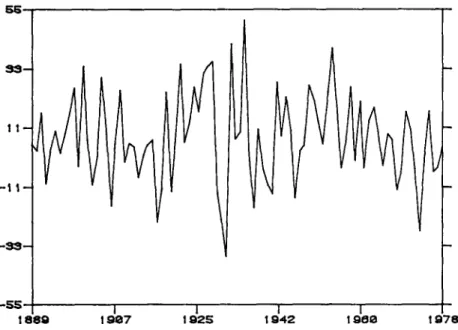
Fig. 1. Real annual return on S&P 500, 1889-1978 (percent).
1920-1930 period and sixty-day to ninety-day Prime Commercial Paper prior to 1920. 4
These series were used to generate the series actually utilized in this paper. Summary statistics are provided in table 1.
Series P and D above were used to determine the average annual real return on the Standard and Poor's 500 Composite Index over the ninety-year period of study. The annual return for year t was computed as (Pt+x + D t - P t ) / P t • The returns are plotted in fig. 1. Series C was used to determine the process on the growth rate of consumption over the same period. Model parameters were restricted to be consistent with this process. A plot of the percentage growth of real consumption appears in fig. 2. To determine the real return on a relatively riskless security we used the series R F and P C . For year t this is calculated to be R F t - ( P C , + 1 - P C t ) / P C , .
This series is plotted in fig. 3. Finally, the Risk Premium (R.P) is calculated as the difference between the Real Return on Standard and Poor's 500 and the Real Return on a Riskless security as defined above.
P~ Mehra and E.C. Prescott, The equity premium 149
l S
1 8 8 9 1 9 ~ 7 ] 1 9 2 S l 1 9 4 2 I 1 9 0 9 1
Fig. 2. Growth rate of real per capita consumption, 1889-1978 (percent).
1 9 7 8
11
- 1 1 -
- S 3 -
t
- S S I 1 I 1
1 8 8 9 1 9 9 7 1 9 2 5 1 9 4 2 1.91~8 1 9 7 8
I
150
R. Mehra and E.C. Prescott, The equity premium3. The economy, asset prices and returns
In this paper, we employ a variation of Lucas' (1978) pure exchange model. Since per capita consumption has grown over time, we assume that the growth
rate of the endowment follows a Markov process. This is in contrast to the
assumption in Lucas' model that the endowment leoel follows a Markov process. Our assumption, which requires an extension of competitive equi- librium theory, enables us to capture the non-stationarity in the consumption series associated with the large increase in per capita consumption that occurred in the 1889-1978 period.
The economy we consider was judiciously selected so that the joint process governing the growth rates in aggregate per capita consumption and asset prices would be stationary and easily determined. The economy has a single representative 'stand-in' household. This unit orders its preferences over ran- dom consumption paths by
,/
F.o ,
O)
where c, is per capita consumption, /~ is the subjective time discount factor, E0{. } is the expectation operator conditional upon information available at time zero (which denotes the present time) and U: R+--* R is the increasing concave utility function. To insure that the equilibrium return process is stationary, the utility function is further restricted to be of the constant relative risk aversion class,
c 1-a - 1
U(c,a)= 1 - a ' O<a<oo. (2)
The parameter a measures the curvature of the utility function. When e( is equal to one, the utility function is defined to be the logarithmic function, which is the limit of the above function as a approaches one.
We assume that there is one productive unit producing the perishable consumption good and there is one equity share that is competitively traded. Since only one productive unit is considered, the return on this share of equity is also the return on the market. The firm's output is constrained to be less than or equal to Yr It is the firm's dividend payment in the period t as well.
The growth rate in y, is subject to a Markov chain; that is,
R. Mehra and E.C. Prescott, The equity premium 151
where xt+ 1 E ( h 1 .. . . . hn} is the growth rate, and
Pr{ xt+ 1 = hi; x, = hi} = ~/j. (4)
It is also assumed that the Markov chain is ergodic. The h i are all positive and
Yo > 0. The random variable Yt is observed at the beginning of the period, at
which time dividend payments are made. All securities are traded ex-dividend.
We also assume that the matrix A with elements aiy = [~dPijh~ r'a for i, j =
1 . . . n is stable; that is, lira A m as m ~ co is zero. In Mehra and Prescott
(1984) it is shown that this is necessary and sufficient for expected utility to
exist if the stand-in household consumes Yt every period. They also define and
establish the existence of a Debreu (1954) competitive equilibrium with a price system having a dot product representation under this condition.
Next we formulate expressions for the equilibrium time t price of the equity share and the risk-free bill. We follow the convention of pricing securities ex-dividend or ex-interest payments at time t, in terms of the time t consump- tion good. For any security with process { d, } on payments, its price in period t is
P t = E t { ~ ,
fl'-tU'(y,)dJU'(Yt)},
s - - t + l
(5)
as equilibrium consumption is the process (y~) and the equilibrium price system has a dot product representation.
The dividend payment process for the equity share in this economy is { Ys }-
Consequently, using the fact that U'(c) = c -a,
e, e = P e ( x,, y,)
oo y , }
= E ~ a s - t ,- .-~,r,, t, Yt t x . (6)
s - - t + l Ys
Variables x t and Yt are sufficient relative to the entire history of shocks up
to, and including, time t for predicting flae subsequent evolution of the economy. They thus constitute legitimate state variables for the model. Since
Ys = Y t " x t + t . . . x s, the price of the equity security is homogeneous of degree
one in Yt, which is the current endowment of the consumption good. As the
equilibrium values of the economies being studied are time invariant ftmetions
of the state ( x t, Yt), the subscript t can be dropped. This is accomplished by
152 K Mehra and E.C. Prescott, The equity premium
convention, the price of the equity share from (6) satisfies
/I
- a • C~j ] C a.
pe(c,i)ffl E ¢kij(A, c) [p (hjc, j)+
(7)j - 1
Using the result that
pe(c,i)
is homogeneous of degree one in c, werepresent this function as
p O ( c , i ) = w,c, (8)
where w i is a constant. Making this substitution in (7) and dividing by c yields
wi= fl ~ epijhSl-a)(w j+
1) for i = 1 ... n. (9)j - - 1
This is a system of n linear equations in n unknowns. The assumption that guaranteed existence of equilibrium guarantees the existence of a unique positive solution to this system.
The period return if the current state is (c, i) and next period state (h~c, j ) is
r,~ = Pe(Xjc' j) + >~jc
- p e ( c , i)pe(c,i)
_ X j ( w j + l )
w,. 1, (10)
using (8).
The equity's expected period return if the current state is i is
R =
F., %,;;..
( n )j - 1
Capital letters are used to denote expected return. With the subscript i, it is the expected return conditional upon the current state being (c, i). Without this subscript it is the expected return with respect to the stationary distribution. The superscript indicates the type of security.
R. Mehra and E.C. Prescott, The equity premium
From (6),
p:=p'(c,
i)
=
,,jv,(x:)/u'(c)
j - 1
=
fl
e P u X ~ .j - - 1
153
(12)
The certain return on this riskless security is
R[ = 1 / p : - 1,
(13)when the current state is (c, i).
As mentioned earlier, the statistics that are probably most robust to the modelling specification are the means over time. Let ~r ~ R n be the vector of stationary probabilities on i. This exists because the chain on i has been assumed to be ergodic. The vector ~r is the solution to the system of equations
~r = ~ r r r ,
with
~ r i = l and ~ r = { ~ j , } . i - - 1
The expected returns on the equity and the risk-free security are, respectively,
n
Re= E ~riR: and Rf= ~ ~'iR[.
(14)i - 1 i - 1
Time sample averages will converge in probability to these values given the ergodicity of the Markov chain. The risk premium for equity is R e - R r, a parameter that is used in the test.
4. The results
154 R. Mehra and E.C. Prescott, The equity premium
assume two states for the Markov chain and to restrict the process as follows:
~x=1+~+6, h2=1+~-6,
1#11 = 1#22 = 1#' 1#12 = 1#21 = (1 - 1#).
The parameters g, 1#, and 6 now define the technology. We require 6 > 0 and 0 < 1# < 1. This particular parameterization was selected because it permitted us to independently vary the average growth rate of output by changing g, the variability of consumption by altering 6, and the serial correlation of growth rates by adjusting 1#.
The parameters were selected so that the average growth rate of per capita consumption, the standard deviation of the growth rate of per capita consump- tion and the first-order serial correlation of this growth rate, all with respect to the model's stationary distribution, matched the sample values for the U.S. economy between 1889-1978. The sample values for the U.S. economy were 0.018, 0.036 and -0.14, respectively. The resulting parameter's values were = 0.018, $ = 0.036 and 1# = 0.43. Given these values, the nature of the test is to search for parameters a and fl for which the model's averaged risk-free rate and equity risk premium match those observed for the U.S. economy over this ninety-year period.
The parameter a, which measures peoples' willingness to substitute con- sumption between successive yearly time periods is an important one in many fields of economics. Arrow (1971) summarizes a number of studies and concludes that relative risk aversion with respect to wealth is almost constant. He further argues on theoretical grounds that a should be approximately one. Friend and Blume (1975) present evidence based upon the portfolio holdings of individuals that a is larger, with their estimates being in the range of two. Kydland and Prescott (1982), in their study of aggregate fluctuations, found that they needed a value between one and two to mimic the observed relative variabilities of consumption and investment. Altug (1983), using a closely related model and formal econometric techniques, estimates the parameter to be near zero. Kehoe (1984), studying the response of small countries balance of trade to terms of trade shocks, obtained estimates near one, the value posited by Arrow. Hildreth and Knowles (1982) in their study of the behavior of farmers also obtain estimates between one and two. Tobin and Dolde (1971), studying life cycle savings behavior with borrowing constraints, use a value of 1.5 to fit the observed life cycle savings patterns.
R. Mehra and E.C. Prescott, The equity premium 155
Averac3e
IR,sk Premi8
(percent} Re - R ~
Aclr~,ssL ble Re~ion
0 I ~, 3 N (percent) Avera~3e R~sk Free Rate
Fig. 4. Set of admissible average equity risk premia and real returns.
tion. 5 With a less than ten, we found the results were essentially the same for very different consumption processes, provided that the mean and variances of growth rates equaled the historically observed values. An advantage of our approach is that we can easily test the sensitivity of our results to such distributional assumptions.
The average real return on relatively riskless, short-term securities over the 1889-1978 period was 0.80 percent. These securities do not correspond per- fectly with the real bill, but insofar as unanticipated inflation is negligible a n d / o r uncorrelated with the growth rate x t + 1 conditional upon information at time t, the expected real return for the nominal bill will equal R[. Litterman (1980), using vector autoregressive analysis, found that the innovation in the inflation rate in the post-war period (quarterly data) has standard deviation of only one-half of one percent and that his innovation is nearly orthogonal to the subsequent path of the real G N P growth rate. Consequently, the average realized real return on a nominally denoted short-term bill should be close to that which would have prevailed for a real bill if such a security were traded. The average real return on the Standard and Poor's 500 Composite Stock
156 R. Mehra and E.C. Prescott, The equity premium
Index over the ninety years considered was 6.98 percent per annum. This leads to an average equity premium of 6.18 percent (standard error 1.76 percent).
Given the estimated process on consumption, fig. 4 depicts the set of values of the average risk-free rate and equity risk premium which are both consistent with the model and result in average real risk-free rates between zero and four percent. These are values that can be obtained by varying preference parame- ters a between zero and ten and fl between zero and one. The observed real return of 0.80 percent and equity premium of 6 percent is clearly inconsistent with the predictions of the model. The largest premium obtainable with the model is 0.35 percent, which is not close to the observed value.
4.1. Robustness of results
One set of possible problems are associated with errors in measuring the inflation rate. Such errors do not affect the computed risk premium as they bias both the real risk-free rate and the equity rate by the same amount. A potentially more serious problem is that these errors bias our estimates of the growth rate of consumption and the risk-free real rate. Therefore, only if the tests are insensitive to biases in measuring the inflation rate should the tests be taken seriously. A second measurement problem arises because of tax consider- ations. The theory is implicitly considering effective after-tax returns which vary over income classes. In the earlier part of the period, tax rates were low. In the latter period, the low real rate and sizable equity risk premium hold for after-tax returns for all income classes [see Fisher and Lofie (1978)].
We also examined whether aggregation affects the results for the case that the growth rates were independent between periods, which they approximately were, given that the estimated 4, was near one-half. Varying the underlying time period from one one-hundredths of a year to two years had a negligible effect upon the admissible region. (See the appendix for an exact specification of these experiments.) Consequently, the test appears robust to the use of annum data in estimating the process on consumption.
R. Mehra and E.C: Prescott, The equi(y premium
157
growth rate without varying the first or second moments. The maximal equity premium increased by 0.04 to 0.39 only. These exercises lead us to the conclusion that the result of the test is not sensitive to the specification of the process generating consumption.That the results were not sensitive to increased persistence in the growth rate, that is to increases in ~, implies low frequency movements or non- stationarities in the growth rate do
not
increase the equity premium. Indeed, by assuming stationarity, w~ biased the testtowards
acceptance.4.2. Effects of firm leoerage
The security priced in our model does not correspond to the common stocks traded in the U.S. economy. In our model there is only one type of capital, while in an actual economy there is virtually a continuum of capital types with widely varying risk characteristics. The stock of a typical firm traded in the stock market entitles its owner to the residual claim on output after all other claims including wages have been paid. The share of output accruing to stockholders is much more variable than that accruing to holders of other claims against the firm. Labor contracts, for instance, may incorporate an insurance feature, as labor claims on output are in part fixed, having been negotiated prior to the realization of output. Hence, a disproportionate part of the uncertainty in output is probably borne by equity owners.
The firm in our model corresponds to one producing the entire output of the economy. Clearly, the riskiness of the stock of this firm is not the same as that of the Standard and Poor's 500 Composite Stock Price Index. In an attempt to match the two securities we price and calculate the risk premium of a security whose dividend next period is actual output less a fraction of expected output. Let 0 be the fraction of expected date t + 1 output committed at date t by the firm. Eq. (7) then becomes
p e ( c , i ) = [ ~ dpij(~kjC p e j)-t-C~kj--O C a.
(15)
j - 1
As before, it is conjectured and verified that
pC(c, i)
has the functional formwic.
Substitutingwic
forpC(c, i) in
(15) yields the set of linear equations[
]
158 R. Mehra and E.C. Prescott, The equity premium
As the corporate profit share of output is about ten percent, we set 0 = 0.9. Thus, ninety percent of expected output is committed and all the risk is borne by equity owners who receive ten percent of output on average. This increased the equity risk premium by less than one-tenth percent. This is the case because financial arrangements have no effect upon resource allocation and, therefore, the underlying Arrow-Debreu prices. Large fixed payment commit- merits on the part of the firm do not reverse the test's outcome.
4.3. Introducing production
With our structure, the process on the endowment is exogenous and there is neither capital accumulation nor production. Modifying the technology to admit these opportunities cannot overturn our conclusion, because expanding the set of technologies in this way does not increase the set of joint equilibrium processes on consumption and asset prices [see Mehra (1984)]. As opposed to standard testing techniques, the failure of the model hinges not on the acceptance/rejection of a statistical hypothesis but on its inability to generate average returns even close to those observed. If we had been successful in finding an economy which passed our not very demanding test, as we expected, we planned to add capital accumulation and production to the model using a variant of Brook's (1979, 1982), Donaldson and Mehra's (1984) or Prescott and Mehra's (1980) general equilibrium stationary structures and to perform additional tests.
5. Conclusion
The equity premium puzzle may not be why was the average equity return so high but rather why was the average risk-free rate so low. This conclusion follows if one accepts the Friend and Blume (1975) finding that the curvature parameter a significantly exceeds one. For a = 2, the model's average risk-free rate is at least 3.7 percent per year, which is considerably larger than the sample average 0.80 given the standard deviation of the sample average is only 0.60. On the other hand, if a is near zero and individuals nearly risk-neutral, then one would wonder why the average return of equity was so high. This is not the only example of some asset receiving a lower return than that implied by Arrow-Debreu general equilibrium theory. Currency, for example, is dominated by Treasury bills with positive nominal yields yet sizable amounts of currency are held.
R. Mehra and E.C. Prescott, The equity premium 159
time to be poorer substitutes than consumptions at widely separated dates. Perhaps introducing some features that make certain types of intertemporal trades among agents infeasible will resolve the puzzle. In the absence of such markets, there can be variability in individual consumptions, yet little variabili- ty in aggregate consumption. The fact that certain types of contracts may be non-enforceable is one reason for the non-existence of markets that would otherwise arise to share risk. Similarly, entering into contracts with as yet unborn generations is not feasible. 6 Such non-Arrow-Debreu competitive equilibrium models may rationalize the large equity risk premium that has characterized the behavior of the U.S. economy over the last ninety years. To test such theories it would probably be necessary to have consumption data by income or age groups.
Appendix
The procedure for determining the admissible region depicted in fig. 4 is. as follows. For a given set of parameters #, 8 and ~, eqs. (10)-(14) define an algorithm for computing the values of R e, R r and R e - R f for any (a, fl) pair belonging to the set
x = ( ( a , fl): 0 < a < 10, 0 < fl < 1, and the
existence condition of section 3 is satisfied}.
Letting
Rf=hl(ot, fl) and R e - R f f h 2 ( c t , fl), h: X-* R 2,
the range of h is the region depicted in fig. 4. The function h was evaluated for all points of a fine grid in X to determine the admissible region.The experiments to determine the sensitivity of the results to the period length have model time periods n = 2, 1, 1/2, 1/4, 1/8, 1/16, 1 / 6 4 and 1/128 years. The values of the other parameters are # = 0.018/n, 8 = 0.036/x/n" and = 0.5. With these numbers the mean and standard deviation of annual growth rates are 0.018 and 0.036 respectively as in the sample iaeriod. This follows because ~ = 0.5 implies independence of growth rates over periods. The change in the admissible region were hundredths of percent as n varied. The experiments to test the sensitivity of the results to # consider ~ ffi 0.014, 0.016, 0.018, 0.020 and 0.022, ~ = 0.43 and 8 = 0.036. As for the period length, the growth fate's effects upon the admissible region are hundredths of percent. The experiments to determine the sensitivity of results to 6 set ~ = 0.43, ~ = 0.018 and 8--0.21, 0.26, 0.31, 0.36, 0.41, 0.46 and 0.51. The equity premium varied approximately with the square of 8 in this range.
160 IL Mehra and E.C. Prescott, The equity premium
Similarly, to test the sensitivity of the results to variations in the p a r a m e t e r ~, we held ~ fixed at 0.036 a n d / z at 0.018 and varied ~ between 0.005 and 0.95 in steps of 0.05. As ~ increased the average equity p r e m i u m declined.
T h e test for the sensitivity of results to higher m o v e m e n t s uses an e c o n o m y with a four-state M a r k o v chain with transition probability matrix
~ / 2 ~ / 2 1 - ~ / 2 1 - ~ / 2 ] ~ / 2 ~ / 2 1 - ~ / 2 1 - ~ / 2
/
1 - ~ / 2 1 - ~ / 2 ~ / 2 ~ / 2 |" 1 - ~ / 2 1 - ~ / 2 ~ / 2 ~ / 2 JT h e values of the ?~ are h 1 = 1 +/~, h2 = 1 +/~ + 8, ~3 = 1 + #, and X4 = 1 +/~ - 8. Values of/~, 8 and ~ are 0.018, 0.051 and 0.36, respectively. This results in the mean, standard deviation and first-order serial correlations of c o n s u m p - tion growth rates for the artificial economy equaling their historical values. W i t h this M a r k o v chain, the probability of above average changes is smaller and m a g n i t u d e of changes larger. This has the effect of increasing m o m e n t s higher than the second without altering the first or second moments. This increases the m a x i m u m average equity p r e m i u m from 0.35 percent to 0.39 percent.
R e f e r e n c e s
Altug, S.J., 1983, Gestation lags and the business cycle: An empirical analysis, Carnegie-Mellon working paper, Presented at the Econometric Society meeting, Stanford University (Carnegie- Mellon University, Pittsburgh, PA).
Arrow, K.J., 1971, Essays in the theory of risk-bearing (North-Holland, Amsterdam).
Brock, W.A., 1979, An integration of stochastic growth theory and the theory of finance, Part I: The growth model, in: J. Green and J. Scheinkman, eds., General equilibrium, growth & trade (Academic Press, New York).
Brock, W.A., 1982, Asset prices in a production economy, in: JJ. McCall, ed., The economics of information and uncertainty (University of Chicago Press, Chicago, IL).
Constaatinides, G., 1982, Intertemporal asset pricing with heterogeneous consumers and no demand aggregation, Journal of Business 55, 253-267.
Debreu, G., 1954, Valuation equilibrium and Pareto optimum, Proceedings of the National Academy of Sciences 70, 588-592.
Donaldson, J.B. and R. Mehra, 1984, Comparative dynamics of an equilibrium, intertemporal asset pridng model, Review of Economic Studies 51, 491-508.
Fisher, L. and LH. Lorie, 1977, A half century of returns on stocks and bonds (University of Chicago Press, Chicago, IL).
Friend, I. and M.E. Blume, 1975, The demand for risky assets, American Economic Review 65, 900-922.
Grossman, S.J. and R.J. Shiller, 1981, The determinants of the variability of stock market prices, American Economic Review 71, 222-227.
t-Iildreth, C. and G.J. Knowles, 1982, Some estimates of Farmers' utility functions, Technical bulletin 335 (Agricultural Experimental Station, University of Minnesota, Minneapolis, M'N). Homer, S., 1963, A history of interest rates (Rutgers University Press, New Brunswick, NJ). Ibbotson, R.O. and R.A. Singuefield, 1979, Stocks, bonds, bills, and inflation: Historical returns
R. Mehra and E.C. Prescott, The equity premium 161 Kehoe, P.J., 1983, Dynamics of the current account: Theoretical and empirical analysis, Working
paper (Harvard University, Cambridge, MA).
Kydland, F.E. and E.C. Prescott, 1982, Time to build and aggregate fluctuations, Econometrica 50,
1345-1370.
LeRoy, S.F. and CJ. LaCivita, 1981, Risk-aversion and the dispersion of asset prices, Journal of" Business 54, 535-548.
LeRoy, S.F. and R.D. Porter, 1981, The present-value relation: Tests based upon implied variance bounds, Econometrica 49, 555-574.
Litterman, R.B. 1980, Bayesian procedure for forecasting with vector autoregressious, Working paper (M.IT, Cambridge, MA).
Lucas, R.E., Jr., 1978, Asset prices in an exchange economy, Econometrica 46, 1429-1445. Lucas, R.E., Jr., 1981, Methods and problems in business cycle theory, Journal of Money, Credit,
and Banking 12, Part 2. Reprinted in: R.E. Lucas, Jr., Studies in business-cycle theory (M1T Press, Cambridge, ]viA).
Mehra, R., 1984, Recursive competitive equilibrium: A parametric example, Economics Letters 16, 273-278.
Mehra, R. and E.C. Prescott, 1984, Asset prices with nonstationary consumption, Working paper (Graduate School of Business, Columbia University, New York).
Merton, R.C., 1973, An intertemporal asset pricing model, Econometrica 41, 867-887.
Prescott, E.C. and R. Mehra, 1980, Recursive competitive equilibrium: The case of homogeneous households, Econometrica 48, 1365-1379.
Shiller, R3., 1981, Do stock prices move too much to be justified by subsequent changes in dividends?, American Economic Review 71,421-436.
Tobin, J. and W. Dolde, 1971, Wealth, liquidity and consumption, in: Consumer spending and monetary policy: The linkage (Federal Reserve Bank of Boston, Boston, MA) 99-146. Wallace, N., 1980, The overlapping generations model of fiat money, in: J.H. Kareken and 1'4.