Do Borrowing Constraints Decrease
Intergenerational Mobility?
Evidence from Brazil
EDUARDO ANDRADE FERNANDO VELOSO
[email protected] [email protected]
Ibmec – SP Ibmec – RJ
REGINA MADALOZZO SERGIO G. FERREIRA
[email protected] [email protected]
Ibmec – SP BNDES
Abstract
In this paper, we find evidence that suggests that borrowing constraints may be an
important determinant of intergenerational mobility in Brazil. This result contrasts
sharply with studies for developed countries, such as Canada and the US, where credit
constraints do not seem to play an important role in generating persistence of inequality.
Moreover, we find that the social mobility is lower in Brazil in comparison with
developed countries.
We follow the methodology proposed by Grawe (2001), which uses quantile
regression, and obtain two results. First, the degree of intergenerational persistence is
greater for the upper quantiles. Second, the degree of intergenerational persistence
declines with income at least for the upper quantiles. Both findings are compatible with
the presence of borrowing constraints affecting the degree of intergenerational
I. Introduction
In the last decade, several studies have attempted to estimate the degree of
intergenerational mobility of economic status across families, both in developed and in
developing countries.1 One of the most widely used economic theories of
intergenerational mobility is based on the existence of intergenerational borrowing
constraints.
Several studies have analyzed the role of borrowing constraints in generating
persistence of income status across generations.2 The main idea is that credit constraints
tend to increase persistence to the extent that investments in children among constrained
families depend on family resources. This creates a link between income of parents and
children in addition to any possible income correlation that may result from the
transmission of ability across generations.
The most widely used approach is to estimate nonlinear regressions of log child's
income when adult on log father's income.3 Implicit in these studies is the assumption
that regression would be linear in the absence of borrowing constraints. The nonlinearity
is assumed to capture the fact that the constraint is less binding at different levels of
father's income than at others.
One problem with this approach is that, as Grawe (2001) shows, depending on
how unobservable ability affects wages, nonlinearities may result even in the absence of
borrowing constraints. Moreover, borrowing constraints are consistent with any nonlinear
pattern, depending on how constrained families are distributed across income classes.
1
For recent evidence on developed countries, see Mulligan (1997) and Solon (1999), for the United States, Bjorklund and Jantti (1997), for Sweden, Dearden, Machin and Reed (1997), for Great Britain, Couch and Dunn (1997), for Germany, and Corak and Heisz (1999), for Canada. Solon (2002) presents evidence for several developed countries. Earlier studies include Behrman and Taubman (1990), Solon (1992) and Zimmerman (1992). For evidence on developing countries, see Lillard and Kilburn (1995), for Malaysia, Hertz (2001), for South Africa, Ferreira and Veloso (2003) for Brazil, and Birdsall and Graham (2000) and Behrman, Gaviria e Szekély (2001) for several Latin American countries. Grawe (2001) presents evidence for several developed and developing countries.
2
See, for example, Loury (1981), Becker and Tomes (1986), Mulligan (1997), Grawe (2001) and Grawe and Mulligan (2002).
3
In this paper, we implement a test of the presence of borrowing constraints using
quantile regression, which was proposed by Grawe (2001). He shows that nonlinear
regressions on the mean may be augmented by quantile regressions to better evaluate
whether borrowing constraints can account for the observed nonlinearities in income
regression.
The main idea is that an increase in child's ability results in a higher level of the
efficient human capital, which makes it more likely for the family to be constrained.
Since children in the highest quantiles tend to have higher ability, this implies that their
parents will be more likely to be constrained. Hence, we would expect that the
constrained families are the ones in the highest quantiles.
This reasoning suggests that, if observed nonlinearities at the mean regression
result from borrowing constraints, then such nonlinearities must be evident in the upper
quantiles, but not in the lower quantiles. Moreover, since income persistence is stronger
among the constrained than the unconstrained, persistence will be higher in upper
quantiles than in lower ones.
The empirical analysis is implemented for Brazil, using the mobility supplement
of the PNAD 1996, a Brazilian household survey. The PNAD is a suitable data set for our
purposes mainly for two reasons. First, it allows for a study of intergenerational
persistence of economic status for a large developing country. Second, and particularly
important for our purposes, the large number of observations of the PNAD allows for the
estimation of nonlinear mean and quantile regressions, which are crucial for
implementing the test for the presence of borrowing constraints proposed in Grawe
(2001).
The mobility supplement of the PNAD 1996 provides information on the
education and occupation of the household head's father, but it does not give information
on the father's income. In order to construct a measure of father's income, we use a
methodology proposed by Angrist and Krueger (1992) and Arellano and Meghir (1992)
and applied by Bjorklund and Jantti (1997) to the study of intergenerational mobility.
We find that the degree of intergenerational persistence of income in Brazil is
higher than the one observed for developed countries. We also find some weak evidence
declines with income. In order to test for the presence of borrowing constraints, we first
perform quantile linear regressions. We find that persistence is higher at the upper
quantiles, as predicted by the theory. Moreover, the concave pattern observed at the mean
is only evident at the upper quantiles, which is also consistent with the model. The
evidence thus suggests that borrowing constraints may be an important determinant of
intergenerational mobility in Brazil.
The paper is organized as follows. In Section II we present the standard model of
intergenerational borrowing constraints. In Section III we describe the empirical
methodology and the PNAD data set. Section IV presents our empirical results, and
Section V concludes.
II. A Model of Intergenerational Borrowing Constraints
In this section, we present a model of intergenerational borrowing constraints
based on Grawe (2001).4 We assume that a family lives for two generations. Each family
is composed of a father and a son. The father is endowed with ability af and schooling level hf, which produce wage income w a h
(
f, f)
. The father also has access to financial assets xf .Parental investments in the child may take two forms. One possibility is to invest
in the child's human capital, hs. The other alternative is to invest in physical assets, xs, which earn interest at rate r. The parent solves
(
)
(
)
(
) (
)
max ,
. .
,
, 1
0
f s
f s s f f f
s s s s
s
U c c
s t
c h x w a h x
c w a h r x
x
+ + = +
= + +
≥
(1)
4
where af is the ability of the son and cf and cs are the consumption of the father and the son, respectively. The restriction xs ≥0 captures the assumption that parents cannot borrow to finance human capital investments in their children.
For some families, the constraint xs ≥0 does not bind. Assuming there are diminishing returns to the investment in human capital
(
whh <0)
, parents will invest in physical assets and child's human capital in order to equate the marginal returns to thetwo forms of investment
(
,)
1h s s
w h a = +r (2)
From equation (2), we can determine the amount of efficient investment in human
capital as a function of child's ability and the interest rate, hs =h a r
(
s,)
. If ability increases the productivity of human capital investments(
wha >0)
and the interest rate earned on assets is common to all parents, high-ability children will be given morehuman capital than low-ability children, that is, ha >0.
5
The important point to note is that, for unconstrained families, human capital
investments do not depend directly on parental income. As a result, child's earnings do
not depend directly on parental income in general and parent's earnings in particular,
among unconstrained families.
For some families, however, the constraint xs ≥0 will bind. The first-order condition when the borrowing constraint binds is
(
,) (
1)
0
h s s
s
w h a r
U µ
µ
= + +
>
(3)
5
where s
s U U
c ∂ =
∂ and µ is the Lagrange multiplier on the borrowing constraint. From (3),
we can make two important observations. First, comparing with (2), we can observe that,
since the opportunity cost of investing in the human capital of children of equal ability is
higher for constrained than for unconstrained families, the latter will make larger human
capital investments. Second, since µ and Us depend on family resources, human capital investments will depend on family income among constrained families. As a result,
child's earnings depend directly on parental income in general, and parent's earnings in
particular, among constrained families.
The model described above thus has the following implication. If all families have
the same ability, then the degree of intergenerational income transmission, also known as
intergenerational persistence, should be zero for unconstrained families, and strictly
positive for constrained families.
The major difficulty in testing the prediction above results from the fact that
ability is unobservable and varies among families. Suppose, for example, that ability is
transmitted from parents to children according to the following equation
s f a
a =ρa +ε (4)
where E
( )
ε =a 0,( )
2a a
Var ε =σ and 0< <ρ 1.
In this case, since ability is correlated with the wage rate, we would observe an
empirical relationship between child's earnings and parental earnings even for
unconstrained families due to the unobservable transmission of ability from parents to
children. For constrained families, there would be two channels of intergenerational
persistence: ability transmission and borrowing constraints.
If we assume that regression would be linear in the absence of borrowing
constraints, the degree of persistence is given by6
6
( )
(
( )
)
( )
(
)
,
, 0 if the constraint binds
0 otherwise
f f s f
f s f
w w a w
w a w
β γ κ
κ
= +
> =
(5)
where wf denotes father's earnings, a ws
( )
f is the expected ability of the son conditional on father's log earnings, γ is the degree of persistence in the absence of borrowing constraints and κ captures the effects of the borrowing constraint.A higher level of father's earnings relaxes the constraint
(
κ <1 0)
, since there aremore resources available to finance human capital investments. Higher ability of the child
tightens the constraint
(
κ >2 0)
, since an increase in child's ability results in a higher level of the efficient human capital.In order to test for the presence of borrowing constraints, the most widely used
approach is to test for nonlinearities in income regression.7 The nonlinearity is assumed
to capture the fact that the constraint is less binding at different levels of parent's income
than at others. In terms of equation (5), this is expressed by the dependence of κ on wf. One problem with this approach is that, as Grawe (2001) shows, depending on
how ability enters the wage function, one may observe income nonlinearities even in the
absence of borrowing constraints.8 Moreover, borrowing constraints are consistent with
any nonlinear pattern, depending on how constrained families are distributed across
income classes. In order to observe this, we can differentiate β with respect to wf in (5) to obtain
1 2
s
f f
da d
dw dw
β
κ κ
= + (6)
7
As mentioned in the introduction, Behrman and Taubman (1990), Solon (1992), Corak and Heisz (1999) and Grawe (2001) are examples of this approach. See Grawe (2001) for a description of other approaches used in the literature to testing for borrowing constraints.
8
Since there is a positive correlation between son's ability and father's earnings
0
s f da dw
>
, κ <1 0 and κ >2 0, the sign of (6) is indeterminate.
Grawe (2001) shows that quantile regression can augment mean regression to
better evaluate whether borrowing constraints are the explanation for a nonlinearity in
earnings regression.
The intuition is the following. As we observed above, an increase in child's ability
makes it more likely for the family to be constrained. Since children in the highest
quantiles tend to have higher ability, this implies that their parents will be more likely to
be constrained. Hence, we would expect that the constrained families are the ones in the
highest quantiles. In terms of equation (5), we would expect κ to be positive at the upper quantiles and zero at the lower quantiles.
This reasoning suggests that if we find nonlinearity at the mean regression and
such nonlinearity is driven by nonlinearity in upper quantiles, then this is an evidence
consistent with borrowing constraints.9 In addition, if we find that the upper quantiles are
steeper than the lower quantiles, this will be an additional evidence compatible with the
presence of borrowing constraints. Otherwise, if none of these implications are observed,
the credit constraint hypothesis will be less convincing. These implications will be tested
in the empirical section.
III. Methodology and Data
In this section, we outline the tested econometric specifications, present the
two-sample instrumental variable technique and descriptive statistics of our data. If we
assume that the mobility pattern would be linear in the absence of borrowing constraints,
we can derive three implications from the standard model of borrowing constraints. First,
it implies that a regression of log child's income on log father's income will be nonlinear.
Second, since income persistence is stronger among constrained families than for
unconstrained families, persistence will be higher in upper quantiles than in lower
9
quantiles. Third, the nonlinearities observed at the mean should be evident in the upper
quantiles, but not in the lower quantiles.
a) Conditional Expectation and Quantile Estimations:
The econometric model typically used to assess the extent of intergenerational
income mobility is given by
i i f i
s y
y , =α +β , +ε (7)
where ys,i represents the son’s permanent log earnings, yf,i represents the father’s permanent log earnings, β is the elasticity of son’s earnings with respect to the father’s earnings, and εi is a stochastic term with
0 ) ( i =
E ε , 0E(εiyf,i)= , andE(εi2)=σε2.
If E(yf,i)=E(ys,i)=µ, then the parameter β is an inverse measure of the extent of regression toward the mean across generations. For example, if β is 0.5 then a father whose earnings exceed the mean (of father’s income) by 20% expects his son’s earnings
to exceed the mean (of son’s income) by 10%.10 The measure 1−β is the degree of intergenerational mobility.
As indicated in Section II, the persistence parameter β will vary across income levels in the presence of borrowing constraints. In order to test for such possibility, we
can extend Equation (7) to allow a general nonlinear pattern of intergenerational mobility
across father’s income level.
i i f i
s G Y
Y, =α + ( ,)+ε (8)
where G(.) will take a particular form of a quadratic polynomial in our case:
i i f i
f i
s Y Y
Y, =α +β1 , +β2 2, +ε (9)
Since other potential sources of nonlinearity may compete with borrowing
constraints to generate a nonlinear pattern for the conditional expectation, we use a
10
quantile estimation procedure to better evaluate the presence of borrowing constraints as
a key explanation for the low intergenerational mobility in Brazil.
In the same way that OLS measures the effect of explanatory variables on the
conditional mean of the dependent variable, quantile regression measures the effect of the
explanatory variables at any point in the conditional distribution, for example the median,
the 90th percentile, the 10th percentile, and so on. As described by Koenker and Bassett
(1978)11, the estimation is done by minimizing equation (10):
∑
∑
< ∈ ≥ ∈ − − + − ℜ ∈ {: } {: } ) 1 ( min β β β θ β θβ i i i iyi xi
i i x y i i i
i x y x
y k
(10)
where yi is the dependent variable, xi is the k by 1 vector of explanatory variables with the first element equal to unity, β is the coefficient vector, and θ is the quantile to be estimated. The procedure allows the coefficient vector β to vary across quantiles, which is appropriate for the case of testing the presence of borrowing constraints. 12
For each given level of father’s income, one should expect the lowest quantiles
less likely to be constrained than the highest quantiles, as explained in Section II. In such
case, according to equation (5), the intergenerational income persistence coefficient will
be larger for the upper quantiles. Hence, in the presence of borrowing constraints, one
should expect larger persistence estimates for those at the top of the son’s conditional
income distribution.
Nonetheless, there may be other causes of larger persistence at the top of the
distribution, since we do not have information about how ability impacts the wage
equation. The quantile approach allows us to test for the presence of nonlinearity at any
point of the conditional distribution. As Equation (5) and Equation (6) should make clear,
the function κ
()
. may take any particular form depending on how the unknown average ability varies with parental income. In order to test for nonlinearity on income fordifferent quantiles, we estimate equation (9) for each 10% quantile.
11
See also Koenker and Hallock (2001) for new applications of quantile regressions. 12
b) Data and Instrumental Variable Procedure:
Several studies take data on pairs of father and sons´ income and estimate the
parameterβ. Solon (1992) shows that an OLS estimate using annual measures of father’s income yields a downward-inconsistent estimate ofβ. This happens because the annual income is an imprecise measure of parental permanent income. When a panel data is
available, such bias may be reduced by averaging out several years of observations of
father’s income.13
In developing countries, even cross section data containing pairs of sons and
fathers income are rare. This is the case in this paper, since the mobility supplement of
the 1996 PNAD provides information on the education and occupation of the
questionnaire responder’s father, but it does not give information on the responder’s
father’s income. In such situation, the use of an instrument for father’s income may be a
substitute for the actual father’s income. As instruments for father’s permanent income
we use the father’s occupation and education reported by sons.14
One problem we have to control for comes from the fact that the sample moments
needed for the estimator are taken from two different samples. Statistical inference for
such case (two-sample instrumental variable, TSIV) is discussed by Angrist and Krueger
(1992) and Arellano and Meghir (1992), having been applied by Bjorklund and Jäntti
(1997) to estimate intergenerational earnings mobility in Sweden and in the US.
In the first stage, we use data from four waves of PNADs (1976, 1981, 1986, and
1990) to obtain information on father’s income, education and occupation.15 The PNAD
(National Survey of Household Sample) is an annual household survey conducted by the
Instituto Brasileiro de Geografia e Estatística (IBGE).16 It is important to note that these
information are about our “synthetic fathers”, not the fathers of the sons about whom we
have information in the mobility supplement of the 1996 PNAD. We estimate a wage
13
Examples in the literature are Solon (1992) and Zimmerman (1992) for the US. 14
For the asymptotic statistical properties of instrumental variable estimators, see Solon (1992). 15
equation as function of educational and occupational dummies and interactions between
year-of-birth cohorts and those variables.
In the second stage, the coefficients of the estimated wage equation are used to
predict the income of the actual fathers, that is, the fathers of the sons about whom we
have information in the mobility supplement of the 1996 PNAD. These sons reported
their father’s education and occupation when they (the sons) were 15 years old. Plugging
this information (the education and occupation reported by the sons) in the wage function
and using the estimated coefficients in the first step, we are able to find a substitute for
father’s income. Then, we regress the reported son’s wage on the actual father’s fitted
wage variable to obtain the estimate of intergenerational income persistence, using as
control variables four regional dummies, a quadratic polynomial on age, and a dummy
for blacks and mulattos.
c) Construction of Occupational Variable and Descriptive Statistics of the
Sample:
In order to do such TSIV procedure, we had to construct the occupational and
educational variables of the fathers.17 We use six groups of occupational categories,
according to the classification proposed by Valle Silva (1974) and used by Pastore (1979)
and Pastore and Valle Silva (1999) specifically to study intergenerational mobility of
occupation, which is aimed to capture the amount of skills required to perform each
task.18
One of the advantages of working with PNAD is the large number of
observations. The sample used in the first stage contains 253,798 observations (“synthetic
16
The sample is close to a nationally representative sample, though it is not fully representative of rural areas, especially in the region “North” (more sparsely populated).
17
Since the PNAD-1996 does not provide information about the father’s age, we assumed that the father was born twenty years earlier than the son. Grawe (2001) also assumes a twenty year age difference between generations for the US.
18
fathers”). The sample of males who reported father’s education and occupation used in
the second stage contains 25,927.19
Table 1 shows the educational and wage mean for each of occupational
categories. The sample contains 253,798 individuals (“synthetic fathers”). The average
number of years in school varies from 13.1, for individuals classified in the most skilled
occupational group, up to 2 for individuals at the very bottom of the occupational rank.
The hourly wage rata varies even more, from 15.3 Reais per hour to 1 Real per hour,
respectively for the highest and the lowest occupational rank.
Table 1:
Average Education and Real Wage, per occupational category
Category Education Real wage* # indiv. Frequence
High 13.11 15.3 10121 4%
M-S 9.73 9.58 21359 8%
M 8.57 5.22 37025 15%
M-I 4.9 2.73 96051 38%
L-S 3.19 1.63 61377 24%
L-I 2.05 1.07 27865 11%
PNAD 1976, 1981, 1986, 1990
OBS: Education corresponds to the number of years in school, * Father's predicted real wage (R$/hour).
Table 2 shows information on the parent’s occupation and education attainment
contained in the mobility supplement of the 1996 PNAD and the father’s predicted wage,
that is, the result of the second stage described above. Some points in this table are worth
emphasizing. With respect to education, 35% of those sampled have fathers with less
than one year in school, and 86% of the sample reported having fathers with at most 4
years of schooling.
19
Table 2:
Characteristic of Fathers, by schooling group, 1996 PNAD
Father's Unweighted Weighted Mean Occupational Ranking
Schooling N Percentage Wage* High M-S M M-I L-S L-I
0 10,235 35.37 1.10 0.62 2.82 1.69 15.63 41.29 37.95 1-3 8,493 29.30 1.70 1.23 4.25 4.05 31.9 35.49 23.08 4 6,115 21.53 2.60 1.92 6.85 9.82 45.39 25.34 10.68
5-7 816 2.37 2.82 3.39 7.88 12.55 52.35 17.59 6.24
8 1,202 3.62 4.16 3.6 11.24 23.28 47.25 11.29 3.34
9-10 231 0.65 5.58 5.58 19.04 24.77 35.16 10.13 5.32 11 1,257 3.84 6.28 11.17 21.27 31.12 30.19 4.98 1.27 12-15 97 0.32 10.97 12.36 33.19 27.34 21.61 4.94 0.56
16 976 3.00 13.49 49.86 21.18 19.34 7.75 1.19 0.68
Total 29,422 100.00% 2.40 3.27 6.04 7.13 29.37 31.48 22.72 * Father's predicted real wage (R$/hour).
With respect to the father’s occupation, as expected, the father’s occupational
rank captures cognitive skills not necessarily transmitted through formal learning. For
example, 11% of fathers with completed high school education are classified as working
in high skill activities. However, a strong positive correlation between occupational
ranking and school attainment indicates formal requirements to be eligible for higher skill
occupations. Finally, father’s predicted wage is positively correlated to the number of
years in school with some indication of convexity in schooling premium, since
completing college education more than doubles the real hourly wage with respect to
having a complete high school degree.
Table 3 presents some descriptive statistics on intergenerational mobility. One can
see that the son’s occupational rank is highly correlated to father’s education, and this is
likely to be a consequence of the channel through the investment in human capital. The
probability that the individual perform a high-skill demanding task is 40.5% for those
whose father has completed college and just 1.4% for those whose fathers have zero year
in school. Reported wage rates are strongly correlated with father’s education as well.20
20
Table 3:
Characteristics of the Sons, by Father's Schooling (Males Aged 25-64, 1996 PNAD)
Father's Mean Mean Region Occupational Ranks
Schooling Schooling Wage Blacks NE High M-S M M-I L-S L-I
0 3.9 2.7 49.4 27.3 1.4 5.2 6.5 50.0 24.8 12.1
1-3 6.3 4.1 34.4 16.3 4.0 8.7 10.9 53.2 17.8 5.4
4 8.9 6.3 24.2 11.6 8.4 15.2 17.8 44.9 11.5 2.3
5-7 9.6 5.8 30.2 16.3 9.4 13.3 18.8 46.1 9.8 2.6
8 11.0 8.9 25.9 15.4 15.9 19.7 21.2 36.2 6.3 0.7
9-10 12.0 9.8 27.5 21.6 21.2 19.8 25.8 25.4 7.1 0.7
11 12.4 11.3 18.1 15.8 18.9 24.6 24.3 26.6 5.1 0.5
12-15 12.7 15.0 18.1 14.4 25.3 20.5 31.6 17.1 4.1 1.5
16 14.1 15.3 11.4 14.8 40.5 25.8 17.3 13.2 2.7 0.5
* Son's predicted real wage (R$/hour).
IV – Empirical Analysis
In this section, we perform the empirical analysis to check if borrowing
constraints can be seen as a limiting factor to intergenerational mobility in Brazil. First,
we assume the typical econometric model to assess the extent of intergenerational
mobility specified in equation (7), which is characterized by a linear specification, and
run the OLS and quantile regression.21 Then, we assumed the nonlinear pattern of
intergenerational mobility, the quadratic form as in equation (9), and do the empirical
investigation by using the OLS and quantile approaches. The objective is to compare the
results with the predictions of the theory outlined in section II.
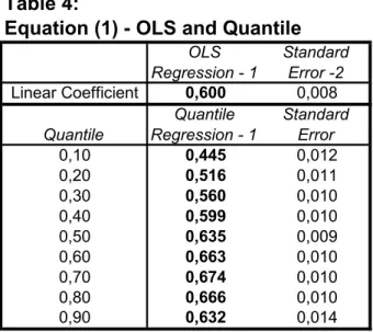
Table 4 and Figure 1 report the results for the OLS and quantile regressions using
the specification in equation (7). The degree of persistence is equal to 0.60 (see the first
line in Table 4) when we use the OLS approach, which is an indication of very low
intergenerational mobility. For example, Mulligan (1997) finds a range from 0.30 to 0.50
for the United States, and Grawe (2001) shows an estimated coefficient lower than 0.30
for Canada.
21
Figure 1
0.3 0.35 0.4 0.45 0.5 0.55 0.6 0.65 0.7 0.75
0.05 0.1 0.15 0.2 0.25 0.3 0.35 0.4 0.45 0.5 0.55 0.6 0.65 0.7 0.75 0.8 0.85 0.9 0.95
Quantile
Estimated Beta
The results obtained with the OLS regression are very different from the ones
found with the quantile approach. Figure 1 shows that there is a significant difference
between the OLS and quantile estimations for the lower quantiles (up to the 25th
percentile) and for the higher quantiles (from the median to the 90th percentile). Mostly
important, however, it is that the degree of persistence varies significantly across Table 4:
Equation (1) - OLS and Quantile
OLS Standard Regression - 1 Error -2
Linear Coefficient 0,600 0,008
Quantile Standard
Regression - 1 Error
0,10 0,445 0,012
0,20 0,516 0,011
0,30 0,560 0,010
0,40 0,599 0,010
0,50 0,635 0,009
0,60 0,663 0,010
0,70 0,674 0,010
0,80 0,666 0,010
0,90 0,632 0,014
Notes:
1 - The coefficients in bold are significant at 95%.
2 - Robust standard errors were calculated using White estimator of variance
quantiles. The pattern is that the degree of persistence increases gradually with the
quantiles, up to the 70th percentile. It ranges from 0.445 for the lowest quantile (10%) to
0.674 for the 70th percentile. The coefficients for the quantiles above 70th percentile are
not significantly different from the one for the 70th percentile.
Hence, there are two important facts coming from the results obtained above.
First, we find nonlinearity in the mean regression that is caused by non-linearity in upper
quantiles. Second, the upper quantiles are steeper than the lower quantiles. As discussed
in Section 2, the combination of these two facts may be explained by the existence of
borrowing constraints. With a greater estimated coefficient for the upper quantiles,
implying less mobility, one can infer that the abler children (and presumably high income
ones), independent of the father’s income, suffer more restriction on their education than
the less able ones. Moreover, this difference in the coefficients for the upper quantiles
with respect to the lower ones would signal a greater intergenerational mobility for the
less able individuals, which do not suffer from credit constraint and the reverse for the
abler individuals, which are more likely to suffer from it. Since children in the highest
quantiles tend to have higher ability, they should receive greater investments in education
and, as a result, their parents are more likely to be constrained. The greater degree of
persistence found for the upper quantiles indicates that the constrained families are more
likely to be the ones in the highest quantiles.
The results obtained above for Brazil contrast sharply with the ones found by
Grawe (2001) for Canada and the United States and Eide and Showalter (1999) for the
United States. They found that, contrary to the prediction of the credit constraint model,
the degree of persistence is greater for the lower quantiles. That is, the lower quantiles are
steeper than the upper quantiles. This difference in the results for Brazil and Canada and
the United States should not come as a surprise. As pointed out by Grawe (2001), the
more developed countries devote a considerable amount of public resources to education
vis-à-vis the less developed ones. Hence, credit constraints may not play an important
role anymore in the education decision in the developed countries.
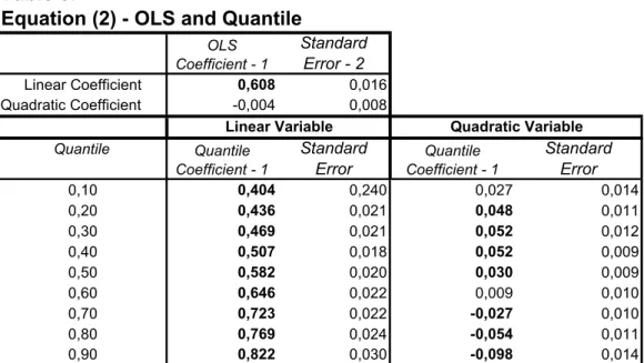
We now turn to the empirical results using the non-linear pattern of
intergenerational mobility, the quadratic form as in equation (9). Table 5 and Figures 2
Figure 2
0.2 0.3 0.4 0.5 0.6 0.7 0.8 0.9 1
0.05 0.1 0.15 0.2 0.25 0.3 0.35 0.4 0.45 0.5 0.55 0.6 0.65 0.7 0.75 0.8 0.85 0.9 0.95
Quantile
Estimated Beta
Table 5:
Equation (2) - OLS and Quantile
Standard Error - 2
Linear Coefficient 0,608 0,016
Quadratic Coefficient -0,004 0,008
Quantile Standard Standard
Error Error
0,10 0,404 0,240 0,027 0,014
0,20 0,436 0,021 0,048 0,011
0,30 0,469 0,021 0,052 0,012
0,40 0,507 0,018 0,052 0,009
0,50 0,582 0,020 0,030 0,009
0,60 0,646 0,022 0,009 0,010
0,70 0,723 0,022 -0,027 0,010
0,80 0,769 0,024 -0,054 0,011
0,90 0,822 0,030 -0,098 0,014
Notes:
1 - The coefficients in bold are significant at 95%.
2 - Robust standard errors were calculated using White estimator of variance
Quantile Coefficient - 1
OLS Coefficient - 1
Linear Variable Quadratic Variable
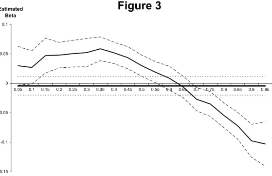
Figure 3
-0.15 -0.1 -0.05 0 0.05 0.1
0.05 0.1 0.15 0.2 0.25 0.3 0.35 0.4 0.45 0.5 0.55 0.6 0.65 0.7 0.75 0.8 0.85 0.9 0.95
Quantile
Estimated Beta
With respect to the degree of persistence, the results are similar to the ones
obtained when the quadratic term was not added in the regression. That is, the pattern of
non-linearity in the mean regression that is caused by non-linearity in upper quantiles and
the fact that the upper quantiles are steeper than the lower quantiles also occur in this new
specification. Hence, the arguments used above that suggest the existence of borrowing
constraint for the families in the highest quantiles are still valid.
With respect to the quadratic term, there is some evidence of a concave pattern,
even though the coefficient on the quadratic term is not statistically significant when we
run OLS. However, when we adopt the quantile approach, most of the quadratic
coefficients are significant for the different quantiles. These are the ones in bold in Table
5. It is interesting to note that the quadratic term is positive for the lower quantiles up to
the 60th percentile, whereas they are negative for the upper quantiles.
Therefore, there is clearly a difference in the non-linear pattern from the upper
quantiles with respect to the lower ones. The concave and convex patterns are observed,
respectively, at the upper and lower quantiles. This pattern change can be seen as an
additional evidence that borrowing constraints may play an important role in explaining
It should be noted that the pattern found for the Brazilian case is very different
from the ones obtained for Canada, Germany, and the United States in Grawe (2001). For
those countries, the upper and lower quantiles have, respectively, convex and concave
patterns.
V. Conclusion
In this paper, we implemented a test to check if borrowing constraints affects the
intergenerational mobility in Brazil. We follow the methodology proposed by Grawe
(2001), which uses quantile regression, and use the database on the mobility supplement
of the 1996 PNAD, a Brazilian household survey.
The main idea is that credit constraints tend to increase persistence to the extent
that investments in children among constrained families depend on family resources. This
creates a link between income of parents and children in addition to any possible income
correlation that may result from the transmission of ability across generations.
If we assume that the mobility pattern would be linear in the absence of
borrowing constraints, we can derive three implications from the standard model of
borrowing constraints. First, it implies that a regression of log child's income on log
father's income will be nonlinear. The nonlinearity captures the assumption that the
constraint is less binding at different levels of father's income than at others.
Second, since income persistence is stronger among constrained families than for
unconstrained families, persistence will be higher in upper quantiles than in lower
quantiles. Third, the nonlinearities observed at the mean should be evident in the upper
quantiles, but not in the lower quantiles.
We tested these implications based on the PNAD data. The mobility supplement
of the PNAD 1996 provides information on the education and occupation of the
household head's father, but it does not give information on father's income. In order to
construct a measure of father's income, we used a methodology recently applied by
The results may be summarized as follows. First, we found evidence of
nonlinearity in the mobility pattern at the mean. In particular, there is some evidence of a
concave pattern, even though the coefficient on the quadratic term is not statistically
significant.
Second, we found that persistence is higher at the upper quantiles than at the
lower quantiles, as predicted by the theory. Third, the concave pattern observed at the
mean is only evident at the upper quantiles, which is also consistent with the model. The
evidence thus suggests that borrowing constraints may be an important determinant of
intergenerational mobility in Brazil.
One result that merits further investigation is that we found a convex mobility
pattern at the lower quantiles. One possible interpretation of this result is that, because of
the way in which ability and education affect wages, the mobility pattern is possibly
convex even in the absence of borrowing constraints.
References
- Angrist, Joshua and Alan Krueger (1992). “The Effect of Age at School Entry on Educational Attainment: An Application of Instrumental Variables with Moments from Two Samples”. Journal of American Statistical Association, 87 (418), p. 328-36. - Arellano, Manuel and Costas Meghir (1992). “Female Labour Supply and On-the-job Search: An Empirical Model Estimated Using Complementary Data Sets”. Review of Economic Studies, 59 (3), p. 537-59.
- Becker, G. and N. Tomes (1986). “Human Capital and The Rise and Fall of Families”. Journal of Labor Economics 4, p. S1-S39.
- Behrman, J, A. Gaviria and M. Székely (2001). “Intergenerational Mobility in Latin America”. Economia, 2 (1), p. 1-44.
- Behrman, J. and P. Taubman (1990). “The Intergenerational Correlation between Children’s Adult Earnings and their Parents’ Income: Results from the Michigan Panel Survey of Income Dynamics”. Review of Income and Wealth 36, p. 115-127. - Birdsall, N. and C. Graham (2000). New Markets, New Opportunities? Economic and
Social Mobility in a Changing World. Washington: Brookings Institution Press and the Carnegie Endowment for International Peace.
- Björklund, A. and M. Jäntti (1997). “Intergenerational Income Mobility in Sweden Compared to the US”. American Economic Review, 87 (5), p. 1009-1018.
- Couch, K. A. and T. A. Dunn (1997). “Intergenerational Correlations in Labor Market Status: A Comparison of the United States and Germany”. Journal of Human Resources, 32, p. 210-32.
- Dearden, L., S. Machin and H. Reed (1997). “Intergenerational Mobility in Britain”. Economic Journal, 107 (440), p. 47-66.
- Eide, E. R. and M. H. Showalter (1999). “Factors Affecting the Transmission of Earnings Across Generations: A Quantile Regression Approach”. Journal of Human Resources, 34 (2), p. 253-267.
- Ferreira, S. G. and F. Veloso (2003). “Intergenerational Mobility of Education in Brazil”, Mimeo. BNDES and Department of Economics, Ibmec.
- Grawe, N. (2001). Intergenerational Mobility in the US and Abroad: Quantile and Mean Regression Measures. Ph.D. dissertation, Department of Economics, University of Chicago.
- Grawe, N. and C. Mulligan (2002). “Economic Interpretations of Intergenerational Correlations”. Journal of Economic Perspectives, 16 (3), p. 45-58.
- Hertz, T. (2001). Education, Inequality and Economic Mobility in South Africa. PhD Thesis, University of Massachusetts.
- Lillard, L. and M. Kilburn. (1995). “Intergenerational Earnings Links: Sons and Daughters”. Mimeo.
- Loury, G. C. (1981). “Intergenerational Transfers and the Distribution of Earnings”. Econometrica, 49 (4), p. 843-67.
- Koenker, R. and Bassett, G. (1978). "Regression Quantiles". Econometrica, Vol. 46, Issue 1, pp. 33-50.
- Koenker, R. and Hallock, K. (2000). “Quantile Regression: An Introduction”, http://www.econ.uiuc.edu/~roger/research/intro/intro.html.
- Koenker, R. and Hallock, K. (2001). “Quantile Regression” Journal of Economic Perspectives, 15, p. 143-56.
- Mulligan, C. (1997). Parental priorities and Economic Inequality. Chicago: University of Chicago Press.
- Mulligan, C. (1999). “Galton versus the Human Capital Approach to Inheritance”. Journal of Political Economy, 107 (6), p. S184-S224.
- Pastore, J. (1979). Desigualdade e Mobilidade Social no Brasil. São Paulo: Editora da Universidade de São Paulo.
- Pastore, J. and N. V. Silva (1999). Mobilidade Social no Brasil. Makron Books. - Solon, G. (1992). “Intergenerational Income Mobility in the United States”. American
Economic Review, 82, p. 393-408.
- Solon, G. (1999). “Intergenerational Mobility in the Labor Market”. In Handbook of Labor Economics, Volume 3A. O. C. Ashenfelter & D. Card, eds. Amsterdam: North-Holland, p. 1761-800.
- Solon, G. (2002). “Cross-Country Differences in Intergenerational Earnings Mobility”. Journal of Economic Perspectives, 16 (3), p. 59-66.
- Valle Silva, N. (1974). Posição Social nas Ocupações. Mimeo, IBGE, Rio de Janeiro. - Zimmerman, D. J. (1992). “Regression Toward Mediocrity in Economic Stature”.