FUNDAC
¸ ˜
AO GETULIO VARGAS
ESCOLA DE P ´
OS-GRADUAC
¸ ˜
AO EM
ECONOMIA
Murilo Esteves de Santi
Assortative Marriage and Intergenerational
Persistence of Earnings: Theory and Evidence
Murilo Esteves de Santi
Assortative Marriage and Intergenerational
Persistence of Earnings: Theory and Evidence
Disserta¸c˜ao submetida a Escola de P´os-Gradua¸c˜ao em Economia como requisito par-cial para a obten¸c˜ao do grau de Mestre em Economia.
Orientador: C´ezar Augusto Ramos Santos
Ficha catalográfica elaborada pela Biblioteca Mario Henrique Simonsen/FGV
Santi, Murilo Esteves
Assortative marriage and intergenerational persistence of earnings: theory and evidence / Murilo Esteves Santi. – 2016.
29 f.
Dissertação (mestrado) - Fundação Getulio Vargas, Escola de Pós- Graduação em Economia.
Orientador: Cézar Augusto Ramos Santos. Inclui bibliografia.
1. Economia - Modelos matemáticos. 2. Teoria dos casamentos. 3. Mercado de trabalho. 4. Renda - Distribuição. I. Santos, Cézar Augusto Ramos. II. Fundação Getulio Vargas. Escola de Pós-Graduação em Economia. III. Título.
CDD – 330.0151
Abstract
I study the impact of the changes in the U.S. labor market that took place in the last
few decades - such as the increase in the college wage premium and the reduction
in the gender wage gap - on the intergenerational persistence of income, with a
particular emphasis on the marriage market channel. To motivate my analysis, I
document a positive cross-country correlation between intergenerational persistence
of income (and education) and educational assortative mating. I then develop an
overlapping generations model in which parents invest in their children’s education
and individuals choose whom they are going to marry, and estimate the model to fit
the postwar U.S. data. My results suggest that both of these changes have affected
the intergenerational earnings persistence, but that the marriage decision plays only
a very small role in these results.
KEYWORDS: Assortative mating, intergenerational persistence of income, gender
Contents
1 Introduction 8
2 Empirical Evidence 11
3 Model 13
3.1 Setup . . . 13
3.2 Human Capital . . . 14
3.3 Preferences . . . 15
3.4 Budget Sets . . . 15
3.5 Recursive Formulation . . . 16
3.6 Government . . . 19
3.7 Steady-State Equilibrium . . . 20
4 Taking the Model to the Data 22 4.1 Parameters Calibrated a Priori . . . 22
4.2 Estimation . . . 22
5 Counterfactual Exercises 25 5.1 Change in the gender wage gap . . . 25
5.2 Change in the skill premim . . . 26
List of Figures
1 Correlation between assortative marriage and intergenerational persistence of income . . . 12 2 Correlation between assortative marriage and intergenerational educational
1
Introduction
In recent years, plenty of empirical studies have documented significant differences in intergenerational earnings elasticity (IGE) between and within countries. This literature has also tried to find socio-economic variables that are correlated with the intergenera-tional persistence of income in order to find its determinants and possible policies that can be implemented in order to guarantee a higher economic mobility between generations. In a famous study, for example,? documented a positive relationship between income in-equality and intergenerational persistence of income - the “Great Gatsby Curve” - at the country level. There are also some papers that found interesting correlations between IGE and socio-economic variables within countries. ?, for instance, found that high mobility areas in the U.S. have less residential segregation, less income inequality, better primary schools, greater social capital, and greater family stability1
. Other socio-economic factors such as union density (?), neighbourhood quality (?, ?), and cultural origins (?) have also been studied in the literature.
Another branch of this empirical literature is concerned with explaining how the marriage market, and in particular the degree of educational assortative mating (the degree to which an individual is more likely to marry someone of the same educational level), may affect the rate of intergenerational mobility. ?, for instance, argued that a high degree of assortative marriage is responsible for the extremely low rates of income mobility in India. ? states that the elevated rate of intergenerational persistence in Chile might be explained by a high degree of assortative mating and ? argued that the rise of income persistence in Catalonia might be the result of the rise in assortative marriage in that region. ?, using U.S. data, find that the intergenerational elasticity between fathers and sons-in-law display a similar trend between 1870 and 1920. ?, using British and German data, finds that about 40-50 percent of the covariance between parents’ and own permanent family income can be attributed to the person to whom one is married.
?, using U.S. data, find that spouse’s earnings are just as elastic as the offspring’s own earnings with respect to the parents’ income2
.
1
? conducted a similar study for Italy and found that higher income mobility is positively correlated with higher value added per capita, higher employment, lower unemployment, higher schooling and higher openness. The authors found no systematic relationship between intergenerational mobility and socio-political outcomes, such as crime and life expectancy.
2
In this paper, I add to this empirical literature by documenting a positive cross-country correlation between educational assortative mating and intergenerational persistence of income. In order to provide a robustness check, I also document a positive cross-country correlation between intergenerational persistence of education and educational assortative mating, with a different sample of countries.
Next, I develop an overlapping generations model in which parents invest in their children human capital and individuals choose whom they are going to marry. I then study how the changes that took place in the U.S. labor market in the postwar period -a lower gender w-age g-ap -and -a higher college w-age premium - h-ave -affected the r-ate of intergenerational mobility, with a particular emphasis on the marriage market channel.
The study of the increase in the college wage premium is motivated by the fact that this process tends to decrease the rate of intergenerational mobility. This happens because, as the college wage premium increases, it gets more costly for a college educated individual to marry a non-college educated one, which should increase the degree of assortative mating. The consequence is that the children of the wealthy parents, which are richer on average because their parents can spend more money in their education, become more likely to get married with a richer spouse.
The effect of the reduction of the gender wage gap in the rate of intergenerational mobility is not clear ex-ante. On the one hand, a lower gender wage gap makes women richer, which allows them to remain single for a longer period of time, and find a highly educated man. If this is the case, then there would be an increase in the degree of marital sorting. On the other hand, a lower gender wage gap makes women more attractive to the men on the marriage market, and men might decide to marry sooner. If this effect dominates, then there would be less assortative mating in the economy. Depending on the direction of the effect, the rate of intergenerational persistence might be higher (if the marital sorting increases), or lower (if it’s the other way around) after a reduction in the gender gape gap.
This paper is also related to a growing quantitative literature concerned with inter-generational mobility and the public policies that can be used to increase it. ? and ?, for example, find that progressive taxation and educational subsidies can substantially reduce the intergenerational persistence of income. ? and ? study how the degree of pro-gressiveness of public education spending affects intergenerational earnings persistence.
? find that geographical differences in skill complementarity account for up to 20 percent of cross-country variation in intergenerational earnings persistence. ? find that fertility differentials and family transfers account for more than 50% of the social mobility in their data.
? also develop an overlapping generations model to study the consequences of a higher degree of assortative mating, but their focus is on long-run inequality and the increase in assortative mating is completely exogenous. While ? builds an overlapping generations model in which the marriage decision is endogenous, their focus is also on income inequality.
? has also studied the changes in the gender wage gap and the college wage premium that occurred in the U.S. in the last decades, but their focus was on how these changes affect divorce rates, college education, income inequality, and married female labor force participation, not intergenerational persistence of income. Moreover, while their model correctly predicted a rise in college enrolment for both men and women in the past 50 years (with a greater increase for women), it was silent about if this increase was the result of a greater college attendance by individuals of rich or poor households. This is particularly important to the study of intergenerational mobility since ? documented that the increase in college completion by women was primarily driven by the rising educational attainment of the daughters of high-income parents, and that this process was not so pronounced among men. By using an overlapping generations model, I will be able to tell if the increase in college attendance in my model is consistent with those findings.
Finally, the two papers that most closely resemble this work are ? and ?. In these works, the authors present an overlapping generations model in which parents invest in their children education and marriage is an endogenous decision. However, their main concern is to study how different antipoverty policies - such as child support, welfare and child tax credits - affect the well being of individuals living in single-parent households. Furthermore, in these models male and female children receive the same amount of edu-cation, which is a supposition that I relax in my model in order to explain the different trends of college attendance by gender that took place in the previous decades.
contributed to reduce it. However, counterfactual analysis in which I hold the educational decision constant and only allow the marriage decision to play a role suggest that the marriage decision played a negligible role in these results.
The rest of this work proceeds as follows. In Section 2 I document a positive corre-lation between intergenerational persistence of income (and education) and educational assortative mating. In Section 3 I describe the model. In Section 4 I discuss the cali-bration procedure. In Section 5 I perform the counterfactual exercises. In Section 6 I conclude and suggest possible extensions to this work.
2
Empirical Evidence
In this section I motivate the quantitative analysis, specially the inclusion of a mar-riage market in a standard overlapping generations model, by documenting a positive cross-country correlation between marital sorting and two measures of intergenerational transmission of economic status.
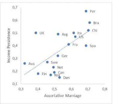
In Figure 1, I plot income persistence in the y-axis against a measure of educational assortative mating in the x-axis. The measure of assortative mating is the correlation between the education of the husband and the wife, in which the education is coded as 1 if the individual has attended at least one year of college or more, and 0 if the individual has only a high-school degree or less. The data for IGE comes from ? and the data for assortative mating comes from ?.
As can be seen in this figure, there is a clear positive relationship between marital sorting and earnings persistence (the correlation is 0.66). In order to verify the robustness of this relationship, I use a measure of intergenerational persistence of education instead of earnings persistence. The data for educational persistence comes from ?.
As can be observed in Figure 2, there is also a positive correlation between educational persistence and assortative mating (in fact the correlation is 0.83, higher than before). Moreover, the sample of countries used in the two measures of persistence is slightly dif-ferent, which allows us to become more confident about the positive relationship between marital sorting and the intergenerational transmission of economic status3
.
3
Both measures contain this same set of countries: Belgium, Brazil, Britain, Denmark, Finland, Italy, Netherlands, Norway, Peru, Sweden, U.S., and Chile. The measure of income persistence also includes Argentina, Australia, Canada, Spain, France, and Germany. The measure of educational persistence includes Colombia, Czech Republic, Ecuador, Hungary, Panama, Poland, and Slovakia
Figure 1: Correlation between assortative marriage and intergenerational persistence of income
Figure 2: Correlation between assortative marriage and intergenerational educational persistence
3
Model
In this section I develop a model of intergenerational transmission of income that explicitly accounts for the role of educational assortative mating. The model adds a marriage decision (modelled in a similar way than in ? and ?) to a standard model of intergenerational earnings persistence (?), whose main features are investments in human capital and innate ability transmission. I’ll keep the notation as close as possible to ?
3.1
Setup
The economy is populated by an equal number of males and females. Each household consists of a father, a mother, and two children of the same gender. A female earns a fraction Φ of what a male with the same education does. Labor is supplied inelastically and is the only source of income (i.e., there is no capital). Individuals live for five periods. In the first period an individual is a child in its parents household. The parents decide how to split their income between consumption and investment in their children’s early education. A higher initial education lowers the disutility of attending college.
In the second period, the individual is a young adult and still lives in its parents’ household. The parents must decide whether or not to send their children to college. Going to college is costly - there is the monetary cost of tuition, the opportunity cost of time, and a psychological cost - but increases the child’s human capital, and the probability of meeting someone who attended college in the marriage market.
In the third period individuals decide whom they are going to marry. There are two rounds. In the first, an agent will randomly meet an individual of the opposite sex and they must decide whether or not to get married (a marriage will only occur if both parts agree). If one of them prefers to remain single, both agents will go to the second round where they will necessarily marry another single individual. There is a higher probability of meeting someone of the same educational level in the second round4
.
Two factors will influence the marriage decision. The economic factor is that marrying a partner with a higher human capital increases the available income of the household. The non-economic factor is a match-specific bliss shock b, which will enter in the utility function in an additively separable way. Given this, the lower the human capital of the the individual one meets in the first round of the marriage market, the higher the bliss shock must be in order to make the marriage decision attractive.
In the fourth period individuals become parents. Both of their children will be male or female with equal probability, and their intrinsic ability will be determined by the intrinsic ability of the parents and a random shock. In this period the parents will determine their children initial education, as described before. In the fifth period the parents decide
4
This assumption is not present in?. The reason behind it is that in my model the marriage market only has two rounds, while in their model there are several. So in order to match the degree of marital sorting in the data it’s necessary to increase the probability of meeting someone with a similar education in the second round.
whether or not to send their kids to college, in the same way outlined above.
3.2
Human Capital
The amount of acquired ability of a child in the end of the first period is determined by its innate abilityπ, the amount of resources that his parents spent in early education,
e, and the amount of public spending in early education, κ. I follow ? and assume the following functional form for the technology of skill formation:
ˆ
π =π(e+κ)γ (1)
I assume that the innate ability of a children is a function of the innate ability of its mother and father and a random term:
log(π′) = ρlog(πm+πf
2 ) +ε (2)
ε∼N(0, σ2
π) (3)
The human capital level of an individual in the second period of her life will be a function of her decision to attend college or not. If she decides to go to college, than her human capital hg2 will be χa, where χ > 1 is the college wage premium, g ∈ {m, f}
denotes the individuals’ gender and a is a positive number. If she decides to not go to college her human capital will simply be a.
In order to capture the life-cycle profile of earnings, I will assume that the human capital of an individual in the third period of her life is hg3 = ξ1h
g
2, and I will also
assume that the human capital of an individual in the fourth and fifth period of her life is hg4 =ξ2h
g
2 and h
g 5 =ξ3h
g
2, respectively.
3.3
Preferences
The momentary utility exhibits constant relative risk aversion (CRRA) over consump-tion.
u(c) = c
1−σ
1−σ (4)
utility of the three periods as adult and the utility of his/her children:
U =
3
X
t=1
βt−1u(c) +β3Uc (5)
where β is the discount factor and Uc is the children’s utility.
3.4
Budget Sets
In the first period as adults (the third period of their lives), individuals must decide whether or not to get married in the first stage of the marriage market. If they decide to get married, they will face the following budget constraint:
c=w(hm3 + Φh
f
3)(1−τ) (6)
wherecis the consumption, wis the wage rate, andhm3 andh f
3 are the human capital
of the male and the female, respectively, Φ is the gender wage gap andτ is the income-tax rate. If an individual chooses to remain single, his/her budget constraint will be:
c=w∆ghg
3(1−τ) (7)
where ∆m = 1 and ∆f = Φ. In the second period as adults, the young parents will
decide how to divide their income between consumption,cy, and investment in the human
capital of their children, e, according to the following budget constraint:
cy +e=w(hm4 + Φh
f
4)(1−τ) (8)
In the third period as adults, parents must decide whether or not to send their children to college. Attending college is costly. I assume that there is a resource cost, f, and that if a child attends college he/she can’t work a fraction n of the time available in the second period. Therefore, if the parents decide not to send their children to college, their resource constraint will be
co=w(hm5 + Φh
f
5 + 2∆
ghg
2)(1−τ) (9)
If the parents decide to send their children to college, they will face the following budget constraint
co+f =w(hm5 + Φh
f
5 + 2∆
ghg
2(1−n))(1−τ) (10)
where hg2 =χa.
3.5
Recursive Formulation
In their first period as adults individuals must decide whom they are going to marry. There are two stages. In the first, an individual of human capital h3 and innate abilityπ
will randomly meet someone of the opposite gender with human capital and innate ability
h∗
3 and π
∗
, respectively. They will receive a bliss shock b and decide if they want to get married or not. They will get married in the first stage if that’s the optimal decision for both of them. If at least one of them doesn’t want to get married, then both of them will meet a single individual of the opposite gender, and will necessarily marry this person. The value function associated with getting married in the first stage,Vg
m, is the following:
Vmg(h3, π, h
∗ 3, π
∗
, b) = c
1−σ
1−σ +b+Eg,π′[Vy(g, π
′
, hm4 , h f 4)|π, π
∗
] (11)
s.t.
c=w(hm3 + Φh
f
3)(1−τ)
log(π′) = ρlog(πm+πf
2 ) +ε
ε∼N(0, σ2
π)
The value function associated with remaining single in the second stage, Vg s , is
Vsg(hg3, π, te) =
c1−σ
1−σ +
X
g=m,f
1 2 Z ⋄ Z T
Vy(g, π
′
, h4, h
∗ 4)dSˆ
g∗
te(π ∗
, h∗3, te ∗
)dΠ(π′|π, π∗) (12)
s.t.
c=w∆ghg3(1−τ)
log(π′) = ρlog(πm+πf
ε∼N(0, σ2π) Where ˆSteg∗(π∗
, h∗
3, te ∗
) is the distribution of single people from the opposite gender that a single individual with educational level tewill draw his/her mate from, which will be discussed in the next section, and T is the set of possible combinations of ability, hu-man capital and college attendance decision. Notice that, since individuals face different probabilities of meeting a college educated mate in the second stage according to their decision to attend college or not, te must be included as a state variable in the single individuals’ value function. A marriage will take place if and only if:
Vmg(h3, π, h
∗ 3, π
∗
, b)≥Vsg(h3, π, te) and Vg
∗
m (h ∗ 3, π
∗
, h3, π, b)≥Vg
∗
s (h ∗ 3, π
∗
, te∗) (13)
Notice that a marriage will only occur if its optimal for both parties. Let the indicator function 1g(h3, π, te, h
∗ 3, π
∗
, te∗, b) take a value of 1 if both parties in the match prefer to get married and a value of zero otherwise.
1g(h3, π, te, h
∗ 3, π
∗
, te∗, b) =
1, if (13) holds 0, otherwise
(14)
Therefore, the value function of an individual in his/her first period as an adult will be the following:
V(h3, π, te, h
∗ 3, π
∗
, te∗, b) = 1g(h3, π, te, h
∗ 3, π
∗
, te∗, b)Vmg(h3, π, h ∗ 3, π
∗
, b)
+(1−1g(h3, π, te, h
∗ 3, π
∗
, te∗, b))Vsg(h3, π, te) (15)
In their second period as adults, individuals are young parents. Their state variables are the human capital of the father and the mother, and the gender and innate ability of their children. Formally, the young parents solve the following Bellman problem:
Vy(g, π, hm4 , h
f
4) = max cy,e
{ c
1−σ y
1−σ +βVo(g, π,π, hˆ
m 5 , h
f
5)} (16)
s.t.
cy +e=w(hm4 + Φh
f
4)(1−τ)
ˆ
π =π(e+κ)γ
I denote bydy(g, π, hm4 , h f
4) the decision rule for early education spending. In the last
period of their lives, individuals are old parents. They have one more state variable than the young parents, which is the acquired ability of their children, which is necessary to determine their children’s disutility of attending college. It’s also necessary to keep the innate ability of their kids as a state variable because it will help to determine the innate ability of their grandchildren. The old parents solve the following functional equation
Vo(g, π,π, hˆ m5 , h
f
5) = max{V hs
o , Vocoll} (17)
where Vhs
o is the value function associated with not attending college:
Vohs(g, π,π, hˆ m5 , h
f
5) = max co
{ c
1−σ o
1−σ+β
Z
B Z
T
V(h3, π, te, h
∗ 3, π
∗
, te∗, b)dAg∗(π∗, h∗3, te ∗
)dF(b)}
(18)
s.t.
co=w(hm5 + Φh
f
5 + 2∆
ghg
2)(1−τ)
hgy =a
te= 0
whereAg∗
(π∗
, h∗
3, te ∗
) is the distribution of individuals of the opposite gender by abil-ity, human capital, and college attendance, and Vocoll, the value function associated with
attending college, is given by
Vocoll(g, π,π, hˆ m5 , h f
5) = max co
{ c
1−σ o
1−σ−
λg
ˆ
π +β
Z
B Z
T
V(h3, π, te, h
∗ 3, π
∗
, te∗, b)dAg∗(π∗, h∗3, te ∗
)dF(b)}
(19)
s.t.
co+f =w(hm5 + Φh
f
5 + 2∆
ghg
2(1−n))(1−τ)
te= 1 where λg
ˆ
π is the disutility of attending college, which is gender specific and decreasing
in the amount of acquired ability in the previous period, andte is a dummy variable that determines whether or not the children completed the tertiary education. I denote by
do(g, π,π, hˆ m5 , h f
5) the policy rule for college attendance.
3.6
Government
The government uses the income tax revenue to finance its expenditure in early ed-ucation. Let xy ≡(g, π, hm4, h
f
4) and xo ≡ (g, π,π, hˆ m5 , h f
5) denote the state of young and
old parents, respectively, and µy(x4) and µo(x5) their distributions across these states.
The government must, then, respect the following budget constraint:
κ=wτ{
Z
[do(xo)(hm5 + Φh f
5 + 2∆
gχa
(1−n)) + (1−do(xo))(hm5 + Φh f
5 + 2∆
ga
)]dµo(xo)
+
Z
(hm4 + Φh f
4)dµy(xy) + Z
(hm3 + Φh f
3)dM(π, h3, te, π
∗
, h∗3, te ∗
, b)
+
Z
hmy dSm(π, hm3 , te) +
Z
ΦhfydSf(π, hf3, te)} (20)
where M(π, h3, te, π ∗
, h∗
3, te ∗
, b) is the distribution of married individuals, which will be described below. The first term in (20) is the revenue obtained from the old parents and their kids, the second is the revenue obtained from the young parents, the third term is the revenue from the young adults that got married and the fourth and fifth terms are the revenue obtained from male and female individuals that remained single.
3.7
Steady-State Equilibrium
In order solve to their problems, individuals must know the stationary distribution of single individuals of the opposite sex, Sg∗
(π∗
, h∗
y, te ∗
). The non-normalized steady-state distribution for singles is:
Sg(π′, h′3, te ′
) =
Z
B
Z π′,h′3,te′
T
Z
T
(1−1g(h3, π, te, h
∗ 3, π
∗
, te∗, b))dAg∗(π∗, h∗3, te ∗
)dAg(π, h3, te)dF(b)
(21) Now let ˆSg∗
(π∗
, h∗
3, te ∗
) be the normalized distribution for singles of the opposite
gender. It is defined by:
ˆ
Sg∗(π∗, h∗3, te ∗
)≡ S
g∗
(π∗
, h∗
3, te ∗
)
R T dSg
∗
(π∗, h∗ 3, te
∗) (22)
Now let M(π, h3, te, π∗, h∗3, te ∗
, b) be the distribution of married individuals. It’s de-fined by
M(π′, h′3, te ′
, π∗′, h∗3′, te ∗′
, b′) =
Z b′
B
Z π′,h′3,te′
T
Z π∗′,h∗′3 ,te∗′
T
1g(h3, π, te, h
∗ 3, π
∗
, te∗, b)
×dAg∗(π∗, h∗3, te ∗
)dAg(π, h3, te)dF(b) (23)
As mentioned before, individuals meet individuals of the opposite gender in the second round of the marriage market with different probabilities, depending on their decision to attend college or not. Let ˆSteg∗(π∗
, h∗
3, te ∗
) be the probability that an individual of the genderg and college attendance decisionte have of meeting an individual of the opposite gender with human capital h∗
3, innate ability π ∗
, and college level te∗
. Its defined by:
ˆ
Steg∗(π ∗′
, h∗3′, te ∗′
) =
Z π∗′,h∗′3 ,te∗′
T
{1
α1(te6=te
∗
) +θteg[1−1(te6=te ∗
)]}dSˆg∗(π∗, h∗3, te ∗
) (24)
where α is the term that reduces the probability of meeting someone who made a different college decision, and θgte is the term that adjusts the probability of meeting
someone who made the same college decision (by increasing it) in order to guarantee that
R T dSˆ
g∗
te(π ∗
, h∗
3, te ∗
) = 1. It’s defined by:
θgte =
1− 1 α
R
T 1(te 6=te ∗
)dSˆg∗
(π∗
, h∗
3, te ∗
) 1−R
T 1(te6=te ∗
) ˆSg∗
(π∗, h∗ 3, te
∗
) (25)
In words, suppose that among the women that remained single, 30% of them are college educated and 70% are not. Then a college educated male that remained single will meet a woman without college education with probability 0.7
α and will meet a woman
that attended college with probability θm 1 0.3.
Definition 1 A stationary recursive matching equilibrium is a set of value functions for young adults, young and old parents, V, Vy, and Vo, a matching rule for singles, 1g,
parents µo and µy, and distributions of single and married individuals S and M, such
that:
1. The value functionV solves the young adults problem, taking as given the matching rule1g(h
3, π, te, h
∗ 3, π
∗
, te∗, b), the normalized distributions for singlesSˆteg∗(π ∗′
, h∗3′, te ∗′
)for
te= 0,1, and the value function for young parents Vy.
2. The value function Vy solves the young parents problem, taking as given the value
function for old parents, Vo, and the decision rule dy for early education is optimal.
3. The value function Vo solves the old parents problem, taking as given the value
function for young adults, V, and the policy function do for college attendance is optimal.
4. The government budget is balanced. 5. The matching rule 1g(h
3, π, te, h
∗ 3, π
∗
, te∗
, b) is determined in line with (14), taking as given the value functions Vs and Vm.
6. The distributions of young and old parents,µy andµoare stationary and determined
in line with the decision rules for early and college education, dy and do, and with the
matching rule 1g(h
3, π, te, h
∗ 3, π
∗
, te∗
, b).
7. The distributions of single and married individuals, S and M, are determined according to (21) and (23), taking as given the matching rule 1g(h
3, π, te, h
∗ 3, π
∗
, te∗
, b) and the optimal decisions for early and college education, dy and do.
4
Taking the Model to the Data
In this section I describe how the parameter values will be chosen. I will fit the model to the U.S. data of 2005. Some parameter values will be chosen using a priori information and some will be estimated through a minimum distance estimation procedure.
4.1
Parameters Calibrated a Priori
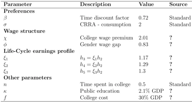
Some of the parameters of the model have a direct empirical counterpart and therefore I can choose their values without solving the model. These parameters areβ, the discount factor, n, the fraction of time spent in college in the second period, σ, the relative risk aversion, Φ, the gender wage gap and χ, the college wage premium. I define the length of a period in the model as 8 years and set β = 0.72 (equivalent to an annual discount factor of 0.96), and n = 0.5 (corresponding to four years of college education). I set
σ = 2, which is in line with the macroeconomic literature. Following ?, I set Φ = 0.83 and χ= 2.01.
I follow ? and set the life-cycle earning profile parameters as ξ1 = 1.17, ξ2 = 1.29,
and ξ3 = 1.3. I also follow ? and define κ, the amount of resources that the government
spends in education, to be equal to 2.1% of GDP. The college cost, f, is set in order to be equal to 30% of GDP, following ?. Table 1 provides a summary of all the parameters chosen using a priori information.
Table 1: Parameters Set Using a Priori Information
Parameter Description Value Source
Preferences
β Time discount factor 0.72 Standard
σ CRRA - consumption 2 Standard
Wage structure
χ College wage premium 2.01 ?
φ Gender wage gap 0.83 ?
Life-Cycle earnings profile
ξ1 h3 =ξ1h2 1.17 ?
ξ2 h4 =ξ2h2 1.29 ?
ξ3 h5 =ξ3h2 1.3 ?
Other parameters
n Time spent in college 0.5 Standard
κ Public education 2.1% GDP ?
f College cost 30% GDP ?
4.2
Estimation
The remaining parameters of the model will be estimated by the Simulated Method of Moments, which consists of minimizing a weighted distance between the model statistics and the data targets. Below I describe which data targets will be more useful to identify each parameter.
Disutility of attending college. The moments that I will use to identify the parameters λm and λf will be the fraction of males and females completing college.
Transmission of heritable traits. The moments that will be used in order to identify the parameters ρ and σπ will be the rate of intergenerational persistence of
Marital sorting. In order to identify the parameters ¯b, σb, and α I will use a
contingency table for marriage which contains the fraction of marriages for each of the four combinations of educational levels for both the husband and the wife.
Human capital production. The parameter γ, which is the elasticity of acquired ability with respect to expenditures, will be chosen to match to share of GDP that is spent in education by private households.
The data used to identify the parameters related to the disutility of attending college and the degree of marital sorting come from ?. I’ll follow ? and define the amount of expenditure in early education by the households as 2.3% of the GDP. The data related to intergenerational persistence of income comes from?, and the data regarding the fraction of children that completed college by their parents income quartile comes from ?. Table 2 summarizes the results of the estimation of the parameters estimated in equilibrium.
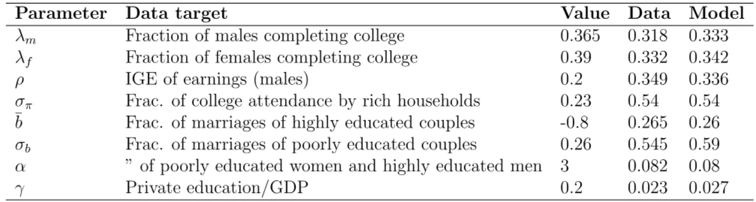
Table 2: Parameters Estimated in Equilibrium
Parameter Data target Value Data Model
λm Fraction of males completing college 0.365 0.318 0.333
λf Fraction of females completing college 0.39 0.332 0.342
ρ IGE of earnings (males) 0.2 0.349 0.336
σπ Frac. of college attendance by rich households 0.23 0.54 0.54
¯b Frac. of marriages of highly educated couples -0.8 0.265 0.26
σb Frac. of marriages of poorly educated couples 0.26 0.545 0.59 α ” of poorly educated women and highly educated men 3 0.082 0.08
γ Private education/GDP 0.2 0.023 0.027
As can be seen in the Table 2, the moments in the model became fairly close to those in the data. The parameter associated with the women disutility of attending college is larger than its male counterpart. The reason for this is that, since the utility function is concave, and the gender wage gap is positive, women receive more utility from the extra income associated with going to college. Since men and women have similar college attendance rates, women must have a higher psychological disutility of attending college in order to justify this data pattern.
The intergenerational earnings elasticity of the male children in the model became fairly close to the one in the data. The intergenerational elasticity of income in the model for female children was of 0.342, which is exactly the same to the one observed in
the data. However, the estimate of the IGE obtained when using the sum of the income of the children and his/her partner is 0.291 in the model, considerably lower than its data counterpart of 0.344. As expected, the IGE estimate obtained when using only the income of the child’s spouse is 0.235, which means that the parents have a higher influence on his/her child income than on his/her child’s partner’s earnings. I’m not aware of any work that has found a data counterpart for this estimative.
The model also did a good job to match the fraction of the children of the parents who belong in the highest income quartile that decided to attend college. However, while in the data 9% of the children whose parents belong in the lowest income quartile completed tertiary education, in my model none of them decided to attend college.
The model was also able to match some of the patterns of marital sorting observed in the data. In particular, it did an excellent job in matching the share of marriages where both partners attended college and the fraction of marriages in which only the husband completed tertiary education. The share of marriages where both individuals did not complete college (and therefore the fraction of marriages in which only the wife is college educated) in the model was a little bit more distant from its data counterpart.
5
Counterfactual Exercises
In this section I will perform two counterfactual exercises. The first is a decrease in the relative wages of women from 83% to 75%. The second is a decrease in the college wage premium from 101% to 90%. In the next two tables, I present the results of the baseline model on the second row and the result of the experiment on the third. On the fourth row I present the results of the experiments when I keep the educational decision constant, and only allow the marriage decision to change. On the fifth row I do the opposite, I fix the marriage decision and only let the individuals change their educational decision.
’Ige of earnings (male)’ is the slope coefficient of a regression of the log of the male children’s income on the log of their parents’ income. ’Ige of earnings (female)’ is the analogous measure for female children. ’Ige of earnings (couple)’ is the slope coefficient of a regression of the log of the sum of the children’s income with his/her partner’s income on the log of their parents income. ’Ige of earnings (couple)’ is the slope coefficient of a regression of the log of the children’s partner’s income on the log of their parents income, i.e., it’s a measure of how much rich parents can increase their children’s earning by helping them to marry a high income partner.
5.1
Change in the gender wage gap
Table 3: Change in the gender wage gap
benchmark change the gwg educ fixed marr fixed
Frac of males completing college 0.333 0.367 0.333 0.367
Frac of females completing college 0.342 0.502 0.342 0.502
single individuals 0.926 0.944 0.926 0.944
ratio of the traces 1.562 1.683 1.562 1.683
IGE of earnings (males) 0.336 0.337 0.336 0.337
IGE of earnings (females) 0.342 0.376 0.342 0.376
IGE of earnings (couple) 0.291 0.298 0.291 0.298
IGE of earnings (spouse) 0.235 0.243 0.235 0.243
private education/GDP 0.027 0.027 0.027 0.027
As can be seen in the Table 3, women tend to go to college at a higher rate when their relative wage is smaller. This occurs because of an income effect: since they are poorer now, some of them decided to go to college in order to mitigate this effect. It can also be seen that more people remain single in the first stage of the marriage market now, this happens because it becomes more costly for a man to marry a non-college educated woman. As a result, the degree of marital sorting increases. The overall effect is that the rate of intergenerational persistence of earnings increases, and this result is almost entirely due to a higher persistence of earnings for women. This occurs because more women are getting college educated, and this increase is concentrated in the daughters of the richest families. It can also be noted that, due to the increase in marital sorting, the parent’s income has a stronger influence in their offspring’s spouse, which also leads to a higher persistence of income.
5.2
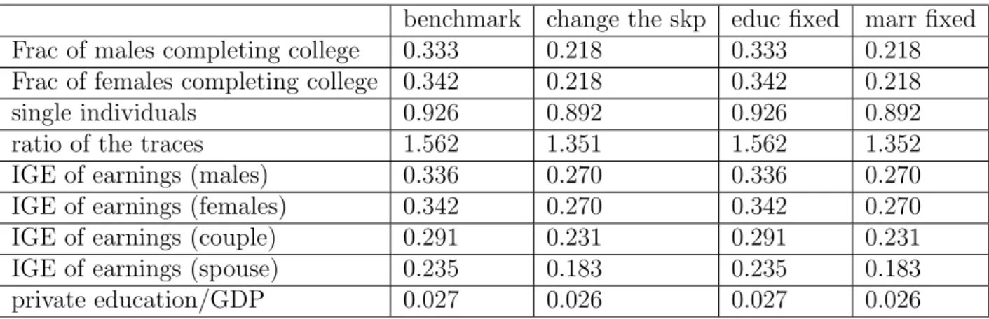
Change in the skill premim
Table 4: Change in the skill premium
benchmark change the skp educ fixed marr fixed
Frac of males completing college 0.333 0.218 0.333 0.218
Frac of females completing college 0.342 0.218 0.342 0.218
single individuals 0.926 0.892 0.926 0.892
ratio of the traces 1.562 1.351 1.562 1.352
IGE of earnings (males) 0.336 0.270 0.336 0.270
IGE of earnings (females) 0.342 0.270 0.342 0.270
IGE of earnings (couple) 0.291 0.231 0.291 0.231
IGE of earnings (spouse) 0.235 0.183 0.235 0.183
private education/GDP 0.027 0.026 0.027 0.026
As can be seen in the table above, when the college wage premium becomes smaller, both men and women reduce their college attendance. It can also be noted that less people are choosing to remain single in the first period, leading to a decrease in marital sorting. This happens because people are less willing to wait for better educated partner, since the monetary gains associated with marrying a college educated individual are now smaller. As a result, the rate of intergenerational transmission of earnings is reduced for two reasons. The first is that since less people are going to college (and this reduction occurs predominantly between the rich households), rich parents are less able to directly affect the income of their offspring. The second is that, since there is less assortative mating, the children of rich parents are less likely to marry college educated individuals, and this also reduces the total income of their family.
6
Conclusion
marriage market played a very small role in these results.
A possible extension to this work would be to include a female labor force participation decision in the model. There has been a remarkable increase in the participation of married woman in the labor market in the previous decades that was not being considered in the model. Importantly, one of the main factors pointed out by the literature as responsible for this increase is the reduction in the gender wage gap5
.
Another possible extension of this work would be to extend the empirical analysis conducted so far by checking if there is also a positive correlation between educational assortative mating and earnings persistence within the U.S. and other countries.
5
See?, for instance.
References
Abbott, B. and Gallipoli, G. Skill Complementarity and the Geography of Intergenera-tional Mobility. working paper, 2015.
Bailey, M. and Dynarski, S. Gains and Gaps: Changing Inequality in U.S. College Entry and Completion. NBER working paper, 2011.
Bruins, M. Cultural Origins and the Geographic Variation in Inter-generational Mobility. working paper, 2016.
Chadwick, L. and Solon, G. Intergenerational Income Mobility among Daughters. The American Economic Review, 2002.
Chetty, R. and Hendren, N. The Impacts of Neighborhoods on Intergenerational Mobility: Childhood Exposure Effects and County-Level Estimates. wp, 2015.
Chetty, R., Hendren, N., Kline, P., and Saez, E. Where is the Land of Opportunity? The Geography of Intergenerational Mobility in the United States. Quarterly Journal of Economics, 2014.
Chetty, R., Hendren, N., and Katz, L. The Effects of Exposure to Better Neighbor-hoods on Children: New Evidence from the Moving to Opportunity Experiment. The American Economic Rebiew, 2015.
Clark, G. The Son Also Rises: Surnames and the History of Social Mobility. Princeton University Press, 2014.
Corak, M. Inequality from Generation to Generation: The United States in Comparison. in Robert Rycroft (editor), The Economics of Inequality, Poverty, and Discrimination in the 21st Century, ABC-CLIO, 2013.
Daruich, D. and Kozlowski, J. Explaining Income Inequality and Social Mobility: The Role of Fertility and Family Transfers. working paper, 2015.
Eckstein, Z. and Lifshitz, O. Dynamic Female Labor Supply. Econometrica, 2011. Ermisch, J., Francesconi, M., and Siedler, T. Intergenerational Mobility and Marital
Fernandez, R. and Rogerson, R. Public Education and Income Distribution: A Dynamic Quantitative Evaluation of Education-Finance Reform. The American Economic Re-view, 1998.
Fernandez, R. and Rogerson, R. Sorting and Long-Run Inequality.The Quarterly Journal of Economics, 2001.
Fernandez, R., Guner, N., and Knowles, J. Love and Money: A Theoretical and Empirical Analysis of Household Sorting and Inequality. The Quarterly Journal of Economics, 2005.
Freeman, R., Han, E., Madland, D., and Duke, B. How Does Declining Unionism Affect the American Middle Class and Intergenerational Mobility.NBER working paper, 2015. Greenwood, J., Guner, N., and Aiyagari, R. On the State of the Union. Journal of
Political Economy, 2000.
Greenwood, J., Guner, N., and Knowles, J. More on Marriage, Fertility, and the Distri-bution of Income. International Economic Review, 2003.
Greenwood, J., Guner, N., Kocharkov, G., and Santos, C. Technology and the Changing Family: A Unified Model of Marriage, Divorce, Educational Attainment and Married Female Labor-Force Participation. AEJ: Macroeconomics, 2015.
Guell, M., Mora, J., and Telmer, C. The Informational Content of Surnames, the Evolu-tion of IntergeneraEvolu-tional Mobility and Assortative Mating.Review of Economic Studies, 2014.
Guell, M., Pellizzari, M., Pica, G., and Mora, J. Correlating Social Mobility and Economic Outcomes. working paper, 2015.
Herrington, C. Public Education Financing, Earnings Inequality, and Intergenerational Mobility. Review of Economic Dynamics, 2015.
Hertz, T., Jayasundera, T., Piraino, P., Selcuk, S., Smith, N., and Verashchagina, A. The Inheritance of Educational Inequality: International Comparisons and Fifty-Years Trends. B.E. Journal of Economic Analysis and Policy (Advances), 2007.
Holter, H. Accounting for Cross-Country Differences in Intergenerational Earnings Per-sistence: The Impact of Taxation and Public Education Expenditure. Quantitative Economics, 2015.
Jones, J. and Yang, F. Skill-Biased Technical Change and the Cost of Higher Education. Journal of Labor Economics, forthcoming, 2016.
Lam, D. and Schoeni, R. Effects of Family Background on Earnings and Returns to Schooling: Evidence from Brazil. Journal of Political Economy, 1993.
Lee, S. and Seshadri, A. On the Intergenerational Transmission of Economic Status. working paper, 2015.
Olivetti, C. and Paserman, M. D. In the Name of the Son (and the Daughter): Intergen-erational Mobility in the United States, 1850-1940. The American Economic Review, 2015.
Restuccia, D. and Urrutia, C. Intergenerational Persistence of Earnings: The Role of Early and College Education. The American Economic Review, 2004.