Comparing solubility algorithms of greenhouse gases in Earth-System modelling

(1)

BGD

12, 15925–15945, 2015

Comparing solubility algorithms of greenhouse gases

V. M. N. C. S. Vieira et al.

Title Page

Abstract Introduction

Conclusions References

Tables Figures

◭ ◮

Back Close

Full Screen / Esc

Printer-friendly Version Interactive Discussion

Discussion

P

a

per

|

Discussion

P

a

per

|

Discussion

P

a

per

|

Discussion

P

a

per

|

Biogeosciences Discuss., 12, 15925–15945, 2015 www.biogeosciences-discuss.net/12/15925/2015/ doi:10.5194/bgd-12-15925-2015

This discussion paper is/has been under review for the journal Biogeosciences (BG). Please refer to the corresponding final paper in BG if available.

Comparing solubility algorithms of

greenhouse gases in Earth-System

modelling

V. M. N. C. S. Vieira1, E. Sahlée2, P. Jurus3,6, E. Clementi4, H. Pettersson5, and M. Mateus1

1

MARETEC, Instituto Superior Técnico, Universidade Técnica de Lisboa, Av. Rovisco Pais, 1049-001, Lisboa, Portugal

2

Dept. of Earth Sciences, Air Water and Landscape sciences, Villavägen 16, 75236 Uppsala, Sweden

3

DataCastor, Prague, Czech Republic

4

Istituto Nazionale di Geofisica e Vulcanologia, INGV, Bologna, Italy

5

Finnish Meteorological Institute, P.O. Box 503, 00101 Helsinki, Finland

6

Institute of Computer Science, Czech Academy of Sciences, Czech Republic

Received: 2 September 2015 – Accepted: 3 September 2015 – Published: 28 September 2015

Correspondence to: V. M. N. C. S. Vieira ([email protected])

(2)

BGD

12, 15925–15945, 2015

Title Page

Tables Figures

◭ ◮

Back Close

Full Screen / Esc

Discussion

P

a

per

|

Discussion

P

a

per

|

Discussion

P

a

per

|

Discussion

P

a

per

|

Abstract

Accurate solubility estimates are fundamental for (i) Earth-System models forecast-ing the climate change takforecast-ing into consideration the atmosphere–ocean balances and trades of greenhouse gases, and (ii) using field data to calibrate and validate the algo-rithms simulating those trades. We found important differences between the formulation

5

generally accepted and a recently proposed alternative relying on a different chemistry background. First, we tested with field data from the Baltic Sea, which also enabled finding differences between using water temperatures measured at 0.5 or 4 m depths. Then, we used data simulated by atmospheric (Meteodata application of WRF) and oceanographic (WW3-NEMO) models of the European Coastal Ocean and

Mediter-10

ranean to compare the use of the two solubility algorithms in Earth-System modelling. The mismatches between both formulations lead to a difference of millions of tons of CO₂, and hundreds of tons of CH₄and N₂O, dissolved in the first meter below the sea surface of the whole modelled region.

1 Introduction

15

Atmosphere–ocean gas exchange is a relevant contemporary subject due to the role of the oceans in the global biogeochemical cycles and their potential as sinks for green-house gases, thus eventually acting as climate change mitigators. In the pole regions, the solubility pump retrieves large amounts of greenhouse gases from the atmosphere and transports them to the deep ocean. On the other hand, the coastal ocean and

20

upwelling zones are traditionally considered as spots of CO2outgassing. These fluxes

of gases across the air–water interface are given by F =kw (Ca/kH−Cw), in units of

mol m−2s−1. Ca and Cw are the air and water gas concentrations in mol m− 3

, kH is

Henry’s constant for the gas specific solubility, here in its scalar (Ca/Cw) form, andkw

the gas transfer velocity across the air–water infinitesimally thin surface layer, in m s−1

25

(3)

BGD

12, 15925–15945, 2015

Title Page

Tables Figures

◭ ◮

Back Close

Full Screen / Esc

Discussion

P

a

per

|

Discussion

P

a

per

|

Discussion

P

a

per

|

Discussion

P

a

per

|

·∆pgas, with ∆pgas being the difference between air and water gas partial pressures

(atm) and kHcp the Henry’s constant in its equivalent Cw/pa form (mol m− 3

atm−1). Frequently, the di_fference between air and water gas concentrations measured in parts-per-million (∆ppm) is used as a proxy for∆pgas. From these formulations can be seen

that, similarly to electric currents or water streams, air–water gas fluxes have two

com-5

ponents: (i) a potential di_fference (unbalance) between two compartments, in this case air and water concentrations, setting a strength and direction of a flux. To this matter, the world oceans, and particularly the coastal oceans, are very heterogenic in their greenhouse gas unbalance with the atmosphere, and with a fine resolution and intri-cacy of processes, associated to upwelling, plankton productivity and continental loads.

10

This holds for CO2 (Smith and Hollibaugh, 1993; Cole and Caraco, 2001; Takahashi

et al., 2002, 2009; Inoue et al., 2003; Duarte and Prairie, 2005; Borges et al., 2005; Rutgersson et al., 2008; Lohrenz et al., 2010; Torres et al., 2011; Oliveira et al.; 2012; Rödenbeck et al., 2013; Schuster et al., 2013; Landschützer et al., 2014; Arruda et al., 2015; Brown et al., 2015) for CH₄(Harley et al., 2015) and for N₂O (Bange et al., 1996;

15

Nevison et al., 1995, 2004; Walter et al., 2006; Barnes and Goddard, 2011; Sarmiento and Gruber, 2013). But an unbalance can also occur within the open ocean at the fine resolution of mesoscale eddies depending on thermodynamic balance, primary pro-ductivity and the time the upwelled water has remained on the surface and departed its cold-core (Chen et al., 2007), or at the larger scale of the Weddell Gyre (Brown

20

et al., 2015). The other component affecting the flux is (ii) the resistance the medium does to being crossed by a flow. The transfer velocity at which gases cross the in-finitesimally thin air–water interface is highly dependent on turbulence upon it. This, in its turn is dependent on its forcings, namely wind drag, wave breaking, currents and rain, and its antagonizers, namely the sea-surface viscosity set by the water

proper-25

(4)

fit-BGD

12, 15925–15945, 2015

Title Page

Tables Figures

◭ ◮

Back Close

Full Screen / Esc

Discussion

P

a

per

|

Discussion

P

a

per

|

Discussion

P

a

per

|

Discussion

P

a

per

|

ted to specific sea-surface conditions or rougher generalizations. In order to calibrate them, the transfer velocities can be estimated from field data reworking the flux equa-tions as:kw=F/(Ca/kH−Cw) orkw=F/(kHcp·∆pgas). The gas flux (F) is measured

in the field with a variety of techniques. The floating dome measures the change in the gas concentration inside a container whose only open side faces the sea-surface

5

(Frankignoulle, 1988). One of the first that used the eddy-covariance method to study the atmosphere–ocean gas fluxes was the COARE experiment (Fairall et al., 1996). Since then, the method has been applied in a growing number of studies (e.g. McGillis et al., 2001, 2004; Rutgersson et al., 2008; Ho et al., 2011). Because the difference in air–water concentrations sets a positive flux downward whereas eddy-covariance

10

methods, being originated from micro-meteorology, traditionally set positive fluxes up-ward, there must be a rectification by−F or−kw in the formulas above (Woolf, 2005;

Zhang et al., 2006). The dual-tracer method, vastly applied to wind tunnel experiments in the late 1970’s–1980’s, can only average a flux over a wide time interval (Watson et al., 1991).

15

AccuratekHestimates are of utmost importance for Earth-System modelling: (i) they

report atmosphere–ocean greenhouse gas equilibrium against which unbalances are estimated, (ii) in dual-layer models, they weight air-side and water-side sea-surface thin layers through which gasses must be transferred, and (iii) they are essential to calibrate air–water gas transfer velocity formulations. Starting in the 1970’s, several

20

authors developed solubility formulations for several gases including the greenhouse gases CO2, CH4 and N2O. Sarmiento and Gruber (2013) compiled a general

algo-rithm together with each gas’ specific constants, to estimate solubility accounting for water temperature, salinity, non-ideal gas behaviour and moisture partial pressure. Re-cently, Johnson (2010) developed an alternative algorithm accounting for temperature,

25

(5)

BGD

12, 15925–15945, 2015

Title Page

Tables Figures

◭ ◮

Back Close

Full Screen / Esc

Discussion

P

a

per

|

Discussion

P

a

per

|

Discussion

P

a

per

|

Discussion

P

a

per

|

included in the Maretec model and software (http://www.maretec.org/en/publications/, <this publication>,<Download zip>) whose development started by Vieira et al. (2013, 2015).

2 Methods

The two formulations were tested with field data from the atmospheric tower at

Öster-5

garnsholm in the Baltic Sea (57◦27′N, 18◦59′E), a Submersible Autonomous Moored Instrument (SAMI-CO₂) 1 km away and a Directional Waverider (DWR) 3.5 km away, both south-eastward from the tower (e.g. Rutgersson et al., 2008 and Högström et al., 2008 for detailed description of the sites). The measurement period was from the 22 to the 26 May 2014. The air–water fluxes were measured by the eddy-covariance method,

10

calculated over 30 min bins and corrected according to the Webb–Pearman–Leuning (WPL) method (Webb et al., 1980). Only the fluxes for which the wind direction set the SAMI-CO₂ and DWR in the footprint of the atmospheric tower (90◦<wind direc-tion<180◦) were used. The SAMI-CO2measured temperature at a depth of 4 m, which

we take as representative for the bulk water temperature. The DWR measured

tem-15

peratures at a depth of 0.5 m, taken here as representative for a closer to sea-surface temperature. The solubility algorithms were tested for the effects of using either tem-perature measurements. Salinity was obtained from the Asko mooring data provided by the Baltic In Situ Near Real Time Observations available in the MyOcean catalogue. The competing formulations were also tested with simulated data relative to the

Euro-20

pean shores from the 24 May 2014 at 06:00 to the 27 May 2014 at 00:00 LT. The air temperature and pressure were retrieved from the lowest level Meteodata.cz standard operational application of the Weather Research and Forecasting Model (WRF) model with 9 km and 1 h resolutions. Over the ocean, the lowest level was never higher than a few centimetres. Sea-Surface Temperature (SST) and salinity (S) were estimated

25

(6)

BGD

12, 15925–15945, 2015

Title Page Abstract Introduction Conclusions References Tables Figures ◭ ◮ ◭ ◮ Back Close

Full Screen / Esc

Printer-friendly Version Interactive Discussion Discussion P a per | Discussion P a per | Discussion P a per | Discussion P a per |

to 20 m depth), 1/12◦_{horizontal and 1 day resolutions. All variables were interpolated to}

the same 0.09◦horizontal grid (roughly 11 km at Europe’s latitude) and 1 h time steps.

2.1 Sarmiento and Gruber (2013) compilation – “Sar13”

The algorithm for temperature and salinity dependence of kHcp provided by Weiss

(1974) and Weiss and Price (1980) has been extensively adapted and applied to other

5

gases. We converted its compilation by Sarmiento and Gruber (2013) to its scalar kH form preserving the ai and bi constants (from their Table 3.2.2) required to esti-mate Bunsen’s solubility coefficient β. This formulation accounted for fugacity (f) of non-ideal gases (Eq. 1) and corrected the gas partial pressure for moisture effects (pmoist=(1−pH₂O/P)pdry) considering water vapour saturation over the sea-surface

10

(Eq. 2). P is air pressure (atm), Tw is water temperature (K), S is salinity (‰), p is

partial pressure (atm), R is the ideal gas law constant (Pa m3mol−1K−1), Vm is the

molar volume of the specific gas (22.3 for CO₂ and CH₄, and 22.2432 for N₂O) and Videal=22.4136 mol L−

1

is the molar volume of ideal gases. Solubility coefficients were estimated from the Virial expansion (Eq. 3), where B was β or β/Vm, depending on

15

which gas it was applied to (see Table 3.2.2 from Sarmiento and Gruber, 2013). The software automatically detected it from theai coefficient. When B=βthekHwas

esti-mated from Eq. (4). When B=β/Vm thekHwas estimated from Eq. (5).

f =exp

_101.325_P₍_V

m−Videal)

RTw

(1) p_H

2O

P =exp

24.4543−67.4509

100 Tw

−4.8489 ln

_T

w

100

−0.000544S

(2)

20

ln (B)=a1+a2

100 Tw

+a3log

Tw

100+a4

_T

w

100

2

+S· b1+b2

Tw

100+b3

_T

w

100

2!

(3)

kH=

1−

pH₂O

P

_101.325_V m

RTwβf

(7)

BGD

12, 15925–15945, 2015

Title Page

Tables Figures

◭ ◮

Back Close

Full Screen / Esc

Discussion

P

a

per

|

Discussion

P

a

per

|

Discussion

P

a

per

|

Discussion

P

a

per

|

kH=

101.325 RTwβf

(5)

2.2 Johnson (2010) formulation – “Joh10”

An extensive list of Henry’s constants in their Cw/pa form was made available by

Sander (1999). These report the solubilities of many gases at 25◦C (298.15 K) and 0 ‰. We used its inverse kHpc (the pa/Cw form), which for CO2 is 29.4, for CH4 is

5

714.3 and for N₂O is 40 L atm mol−1_{. Equation (6) converted}_k

HpctokHat a given

tem-perature and 0 ‰ salinity. The term−∆solnH/R reflected the temperature (in Kelvin)

dependence of solubility (see Sander, 1999), having a value of 2400 for CO2, 1700

for CH₄ and 2600 for N₂O. The correction to a given salinity required a provisional kH#=0.0409·kHpcto estimateθfrom Eq. (7). The liquid molar volume of the gas at its

10

boiling point (Vb) was estimated using the additive Schroeder method. Vb andθwere required to estimate the empirical Setschenow constant Ks=θ·log Vb. Finally,kH,0‰

was corrected for salinity askH=kH,0‰·10 Ks·S_.

k_H,0_‰= 12.1866·kH,pc

P ·Tw·e−

∆SolnH

R (1/Tw−1/298.15)

(6)

θ=7.33532×10−4+3.39615×10−5·log(kH#)−2.40888×10−6·log(kH#)2

15

+1.57114×10−7·log(kH#)3 (7)

3 Results

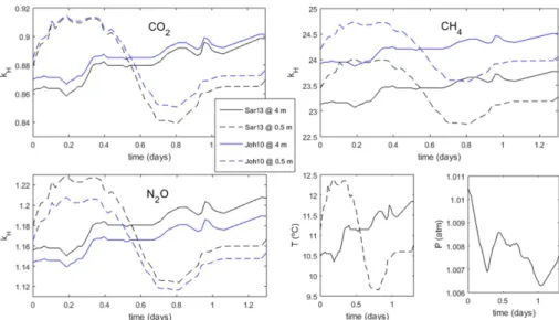
The wind direction set the SAMI-CO₂and the DWR in the footprint of the atmospheric tower only for the first 1.5 days of the experiment, during which the atmospheric pressure and the water temperature vertical profile at the two depths varied (Fig. 1),

20

(8)

BGD

12, 15925–15945, 2015

Title Page

Tables Figures

◭ ◮

Back Close

Full Screen / Esc

Discussion

P

a

per

|

Discussion

P

a

per

|

Discussion

P

a

per

|

Discussion

P

a

per

|

using the algorithms by Johnson (2010) and by Sarmiento and Gruber (2013) fairly matched. Nevertheless, their divergence increased the more the solubility departed from 1 (Fig. 1). This resulted either from: (i) the insoluble nature of the gas, in the case of CH₄, or (ii) the changes in water temperature, in the cases of CO₂ and N₂O. Overall, their roughly 1 % solubility differences when applied to the fairly soluble CO2

5

increased to roughly 3.2 % when applied to the rather insoluble CH4. Far worst

mis-matches occurred between solubilities estimated using water temperatures at the two different depths (Fig. 1), which could go up to 6 % different in the CO2case.

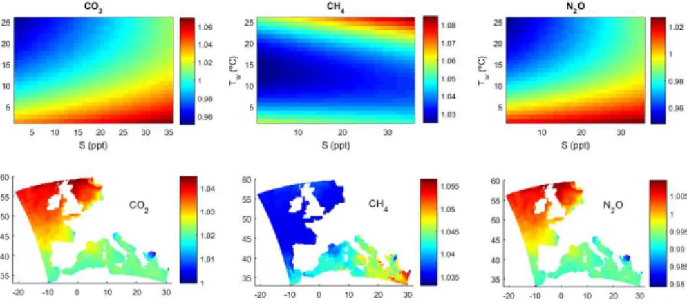
A more thorough perspective of how much both formulations diverge was obtained testingT_wfrom 4 to 30◦C at 1◦C intervals andS from 0 to 36 ppt at 1 ppt intervals, while

10

preserving the remaining environmental conditions as observed during thetinstances the wind blew from the footprint of the atmospheric tower. The formulations were com-pared bykH,Joh10/kH,Sar13, which being a ratio, was averaged overtusing the geometric

mean (Fig. 2). In the cases of CO₂ and N₂O, the two formulations diverge further with saline cooler waters, as occur in the polar regions, and with less-saline warmer waters,

15

as occur in the coastal ocean adjacent to big river estuaries, such as the Amazon, Orinoco, Mississipi, Missouri or Nile. In the case of CH₄, the two formulations diverge more at both temperature extremes.

From the 24 to the 26 May, the water temperature at the first meter below the European coastal ocean surface changed significantly and there was a significant

20

fresh water input from the Black Sea and the Baltic Sea (Video 1). The widest di-vergences in CO2solubility estimates were up to 4.5 % of the solubility and associated

to cooler waters, the widest divergences in the CH₄ solubility estimates were up to 5.8 % of the solubility and associated to both temperature extremes, and the widest divergences in the N2O solubility estimates were up to 2.1 % of the solubility and

as-25

(9)

BGD

12, 15925–15945, 2015

Title Page

Tables Figures

◭ ◮

Back Close

Full Screen / Esc

Discussion

P

a

per

|

Discussion

P

a

per

|

Discussion

P

a

per

|

Discussion

P

a

per

|

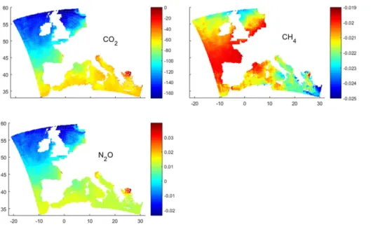
∆t m−1121 km−2=112·∆s·pgas·P ·101 325·Ma/(10 9

·R·T), where∆s was the diff

er-ence in the solubility estimated by either algorithm in itsCw/Caform at each 11 km wide

cells and averaged over the 66 h time interval,Ma=28.97 was the air molecular mass

andpgas was the atmospheric partial pressure of CO2, CH4or N2O, respectively 390,

1.75 and 0.325 ppm (EPA, 2015) under the assumption they were approximately

uni-5

form all over the atmospheric surface boundary layer. The differences alone summed to 3.86×106t of CO2, 880.7 t of CH4and 401 t of N2O. Because the bias of N2O changed

from positive to negative with location, the resulting bias integrated over the whole area was 163 t.

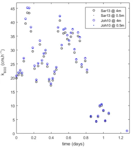
The transfer velocities estimated from the eddy-covariance data showed only small

10

differences. The worst mismatch was a difference (∆k600) of 0.3 cm h− 1

when the trans-fer velocity (k600) was 36 cm h−

1

. The measurements were from the Baltic Sea where the low surface salinity and temperature did not promote much of a difference between thekHestimated by either formulation, and hence did not propagate a mismatch to the

k600estimates. However, simulating a situation with open ocean salinities (35 ppm), the

15

difference∆k600between the two algorithms was around 4.5 % of thek600(Fig. 4). This

difference should increase with lower water temperatures. The effect of water temper-atures measured from different depths was not perceptible.

4 Discussion

Both formulations diverge considerably in their form and background. The Weiss (1974)

20

and Weiss and Price (1980) algorithm, compiled by Sarmiento and Gruber (2013), used the popular Virial equation for an estimation of the effects of temperature and salinity on the Bunsen solubility coefficients. Therefore, their process-oriented description of solubility relies on the ideal gas law. Then, fugacity is estimated to correct for non-ideal gas behaviour, important for gases like CO2, CH4and N2O (Weisenburg and Guinasso,

25

(10)

BGD

12, 15925–15945, 2015

Title Page

Tables Figures

◭ ◮

Back Close

Full Screen / Esc

Discussion

P

a

per

|

Discussion

P

a

per

|

Discussion

P

a

per

|

Discussion

P

a

per

|

the gas atmospheric partial pressure. The formulation by Johnson (2010), an upgrade from Sander (1999), bases its process-oriented description of solubility on the molec-ular structure and thermodynamic properties of the gases. It is remarkable how both algorithms can converge to rather similar results despite their mathematical dissimilar-ities. However, the more uneven are the atmosphere and ocean gas partial pressures

5

at steady state the more divergent are the solubilities estimated by both formulations. This happens either because the gas is rather insoluble or because the ocean sur-face temperature and/or salinity promote that unbalance. This mismatch points out that at least one of the algorithms systematically fails its forecasts, and it can well be both, although this work could not determine which one is it. Nevertheless, within the

10

spatial and time frame of the experiment, this error could lead to a bias of 0.045 mol of CO2 in the ocean surface per mol of CO2 in the atmosphere, 0.0015 mol mol−

1

of CH4 and 0.012 mol mol−

1

of N2O. Furthermore, these biases occur in the most

sensi-tive situations for Earth-System modelling: the cooler waters occur closer to the poles, where the solubility pump traps greenhouse gases and carries them to the deep ocean

15

(Sarmiento and Gruber, 2013); both the warmer waters and the less saline waters oc-cur in the coastal ocean and seas, and there is strong evidence the N₂O dissolved in the coastal ocean is unbalanced with the N2O in the atmosphere (Bange et al., 1996;

Nevison et al., 1995, 2004; Walter et al., 2006; Barnes and Goddard, 2011; Sarmiento and Gruber, 2013). Therefore, the biases of 3.86×106t of CO2, 880.7 t of CH4 and

20

163 t of N2O, estimated for the first meter depth of the European coastal ocean

dur-ing late May 2014, may be an indicator of much higher global biases with stronger consequences. It would not be surprising that former simulations of greenhouse gas exchange between the atmosphere and the world oceans (Nevison et al., 1995, 2004; Walter et al., 2006; Lohrenz et al., 2010; Barnes and Goddard, 2011; Torres et al.,

25

(11)

BGD

12, 15925–15945, 2015

Title Page

Tables Figures

◭ ◮

Back Close

Full Screen / Esc

Discussion

P

a

per

|

Discussion

P

a

per

|

Discussion

P

a

per

|

Discussion

P

a

per

|

ocean represents about 2.4 % of the N₂O yearly discharged by European estuaries, as estimated by Barnes and Goddard (2011). Significant bias in the estimation of the ma-rine N2O dynamics has already been reported (Nevinson et al., 2004; Denman et al.,

2007; Jiang et al., 2007; Barnes and Goddard, 2011). Since marine systems contribute with 10 to 33 % of the tropospheric N2O (Denman et al., 2007; Jiang et al., 2007),

solv-5

ing these potential sources of error is fundamental for a reliable Earth-System model forecasting the climate change. In Parallel, the current coarse resolution Earth-System models, by representing the Earth with approximately 1100 km wide cells, cannot pos-sibly describe with accuracy the solubility heterogeneity that this work demonstrated to occur at the coastal ocean with a fine resolution and high impact in the mass balances

10

of greenhouse gases.

Using the water temperature measured by the DWR at 0.5 m or by the SAMI-CO2

at 4 m depths had a greater impact on the solubility estimates. Unfortunately, it is un-known how much of the temperature di_fferences were due to the di_fferent depths or locations. Nevertheless, it is well known the SST steep vertical gradient originating

15

from the warm-layer and cool-skin effects (Fairall et al., 1996; Zeng and Beljaars, 2005; Brunke et al., 2008). This work proved that a biased SST estimate may propagate to estimates of atmosphere–ocean greenhouse gas trades and balances, and thus the appropriate choices must be made. In order to estimate the atmosphere–ocean un-balanced gas partial pressures, the “warm layer” reporting the average temperature in

20

the first few meters of water seems the obvious choice. However, when weighting the air-side and water-side thin surface layer, the “cool skin” water temperature should be used instead (Fairall et al., 1996; Zeng and Beljaars, 2005; Brunke et al., 2008). The many algorithms estimating the transfer velocity from the sea-surface state and the atmospheric surface boundary layer yield widely divergent results. Many factors

con-25

(12)

BGD

12, 15925–15945, 2015

Title Page

Tables Figures

◭ ◮

Back Close

Full Screen / Esc

Discussion

P

a

per

|

Discussion

P

a

per

|

Discussion

P

a

per

|

Discussion

P

a

per

|

5 Conclusions

For long the Geosciences and Earth-System modelling have accepted the Weiss (1974) and Weiss and Price (1980) formulation as the reliable estimator of solubility. However, its discrepancies with a recent alternative formulation by Johnson (2010) sug-gest this may not be true. Therefore, both formulations need be extensively tested and

5

validated in order to increase accuracy and confidence in the estimates of atmosphere– ocean greenhouse gas exchanges and in the results from Earth-System Models.

The Supplement related to this article is available online at doi:10.5194/bgd-12-15925-2015-supplement.

Author contributions. Software is available at http://www.maretec.org/en/publications/, V. Vieira

10

developed the model and software, analysed the data and wrote the article; E. Sahlée provided the E-C and SAMI data; H. Pettersson provided the Directional Waverider data; P. Jurus pro-vided the WRF data; E. Clementi propro-vided the WW3 data; M. Mateus participated in the model and software development; all co-authors participated in the data analysis and reviewed the article.

15

References

Arruda, R., Calil, P. H. R., Bianchi, A. A., Doney, S. C., Gruber, N., Lima, I., and Turi, G.: Air– sea CO₂fluxes and the controls on ocean surfacepCO₂variability in coastal and open-ocean southwestern Atlantic Ocean: a modeling study, Biogeosciences Discuss., 12, 7369–7409, doi:10.5194/bgd-12-7369-2015, 2015.

20

Bange, H. W., Rapsomanikis, S., and Andreae, M. O.: Nitrous oxide in coastal waters, Global Biogeochem. Cy., 10, 197–207, doi:10.1029/95GB03834, 1996.

Barnes, J. and Upstill-Goddard, R. C.: N₂O seasonal distributions and air–sea exchange in UK estuaries: implications for the tropospheric N₂O source from European coastal waters, J. Geophys. Res., 116, G01006, doi:10.1029/2009JG001156, 2011.

(13)

BGD

12, 15925–15945, 2015

Title Page

Tables Figures

◭ ◮

Back Close

Full Screen / Esc

Discussion

P

a

per

|

Discussion

P

a

per

|

Discussion

P

a

per

|

Discussion

P

a

per

|

Borges, A. V., Delille, B., and Frankignoulle, M.: Budgeting sinks and sources of CO₂ in the coastal ocean: diversity of ecosystems counts, Geophys. Res. Lett., 32, L14601, doi:10.1029/2005GL023053, 2005.

Brown, P. J., Jullion, L. Landschützer, P., Bakker, D. C. E, Garabato, A. C. N., Meredith, M. P., Torres-Valdés, S., Watson, A. J., Hoppema, M., Loose, B., Jones, E. M., Telszewski, M,

5

Jones, S. D., and Wanninkhof, R.: Carbon dynamics of the Weddell Gyre, Southern Ocean, Global Biogeochem. Cy., 29, 288–306, 2015.

Brunke, M. A., Zeng, X., Misra, V., and Beljaars, A.: Integration of a prognostic sea surface skin temperature scheme into weather and climate models, J. Geophys. Res., 113, D21117, doi:10.1029/2008JD010607, 2008.

10

Chen, F., Cai, W.-J., Benitez-Nelson, C., and Wang, Y.: Sea surfacepCO₂-SST relationships across a cold-core cyclonic eddy: implications for understanding regional variability and air– sea gas exchange, Geophys. Res. Lett., 34, L10603, doi:10.1029/2006GL028058, 2007. Cole, J. J. and Caraco, N. F.: Carbon in catchments: connecting terrestrial carbon losses with

aquatic metabolism, Mar. Freshwater Res., 52, 101–110, 2001.

15

Denman, K. L., Brasseur, G., Chidthaisong, A., Ciais, P., Dickinson, R. E., Hauglustaine, D., Heinze, C., Holland, E., Jacob, D., Lohmann, U., Ramachandran, S., da Silva Dias, P. L., Wofsy, S. C., and Zhang, X.: Couplings between changes in the climate system and bio-geochemistry, in: Climate Change 2007: The Physical Science Basis. Contribution of Work-ing Group I to the Fourth Assessment Report of the Intergovernmental Panel on Climate

20

Change, edited by: Solomon, S., Qin, D. Manning, M., Chen, Z., Marquis, M., Averyt, K. B., Tignor, M., and Miller, H. L., Cambridge University Press, New York, 500–587, 2007. EPA United States Environmental Protection Agency – Climate Change Indicators in the United

States – Atmospheric concentrations of greenhouse gases, available at: http://www.epa. gov/climatechange/science/indicators/ghg/ghg-concentrations.html, last accessed: 27

Au-25

gust 2015.

Fairall, C. W., Bradley, E. F., Godfrey, J. S., Wick, G. A., Edson, J. B., and Young, G. S.: Cool-skin and warm-layer e_ffects on sea surface temperature, J. Geophys. Res., 101, 1295–1308, 1996.

Frankignoulle, M.: Field measurements of air–sea CO₂exchange, Limnol. Oceanogr., 33, 313–

30

(14)

BGD

12, 15925–15945, 2015

Title Page

Tables Figures

◭ ◮

Back Close

Full Screen / Esc

Discussion

P

a

per

|

Discussion

P

a

per

|

Discussion

P

a

per

|

Discussion

P

a

per

|

Harley, J. F., Carvalho, L., Dudley, B., Heal, K. V., Rees, R. M., and Skiba, U.: Spatial and sea-sonal fluxes of the greenhouse gases N₂O, CO₂and CH₄in a UK macrotidal estuary, Estuar. Coast. Shelf S., 153, 62–73, 2015.

Ho, D. T., Sabine, C. L., Hebert, D., Ullman, D. S., Wanninkhof, R., Hamme, R. C., Strutton, P. G., Hales, B., Edson, J. B., and Hargreaves, B. R.: Southern Ocean Gas Exchange Experiment:

5

setting the Stage, J. Geophys. Res., 116, C00F08, doi:10.1029/2010JC006852, 2011. Högström, U., Sahlée, E., Drennan, W. M. Kahma, K. K., Smedman, A.-S., Johansson, C.,

Pettersson, H., Rutgersson, A., Tuomi, L., Zhang, F., and Johansson, M.: Boreal Environ. Res., 13, 475–502, 2008.

Inoue, H. Y., Ishii, M., Matsueda, H., Kawano, T., Murata, A., and Takasugi, Y.: Distribution of the

10

partial pressure of CO₂ in surface water (pCOw₂) between Japan and the Hawaiian Islands:

pCOw₂–SST relationship in the winter and summer, Tellus B, 55, 456–465, 2003.

Jiang, X., Ku, W., Shia, R.-L., Li, Q., Elkins, J. W., Prinn, R. G., and Yung, Y. L.: Seasonal cycle of N₂O: analysis of data, Global Biogeochem. Cy., 21, GB1006, doi:10.1029/2006GB002691, 2007.

15

Johnson, M. T.: A numerical scheme to calculate temperature and salinity dependent air–water transfer velocities for any gas, Ocean Sci., 6, 913–932, doi:10.5194/os-6-913-2010, 2010. Landschützer, P., Gruber, N., Bakker, D. C. E., and Schuster, U.: Recent variability of the global

ocean carbon sink, Global Biogeochem. Cy., 28, 927–949, 2014.

Lohrenz, S. E., Cai, W. J., Chen, F., Chen, X., and Tuel, M.: Seasonal variability in air–sea

20

fluxes of CO₂in a river-influenced coastal margin, J. Geophys. Res.-Oceans, 115, C10034, doi:10.1029/2009JC005608, 2010.

Mattia, G., Vichi, M., Zavatarelli, M., and Oddo, P.: The wind-driven response of the Mediter-ranean sea biogeochemistry to the Eastern MediterMediter-ranean Transient. A numerical model study, Geophys. Res. Abstr., 14, EGU2012-4437, 4437 pp., 2012.

25

McGillis, W. R., Edson, J. B., Ware, J. D., Dacey, J. W. H., Hare, J. E., Fairall, C. W., and Wanninkhof, R.: Carbon dioxide flux techniques performed during GasEx-98, Mar. Chem., 75, 267–280, 2001.

McGillis, W. R., Edson, J. B., Zappa, C. J., Ware, J. D., McKenna, S. P., Terray, E. A., Hare, J. E., Fairall, C. W., Drennan, W., Donelan, M., DeGrandpre, M. D., Wanninkhof, R.,

30

(15)

BGD

12, 15925–15945, 2015

Title Page

Tables Figures

◭ ◮

Back Close

Full Screen / Esc

Discussion

P

a

per

|

Discussion

P

a

per

|

Discussion

P

a

per

|

Discussion

P

a

per

|

Nevison, C. D., Weiss, R. F., and Erickson III, D. J.: Global oceanic emissions of nitrous oxide, J. Geophys. Res, 100, 15809–15820, 1995.

Nevison, C. D., Lueker, T. J., and Weiss, R. F.: Quantifying the nitrous oxide source from coastal upwelling, Global Biogeochem. Cy., 18, GB1018, doi:10.1029/2003GB002110, 2004. Oliveira, A. P., Cabeçadas, G., and Pilar-Fonseca, T.: Iberia coastal ocean in the CO₂

5

sink/source context: Portugal case study, J. Coastal Res., 28, 184–195, 2012.

Rödenbeck, C., Keeling, R. F., Bakker, D. C. E., Metzl, N., Olsen, A., Sabine, C., and Heimann, M.: Global surface-ocean pCO₂ and sea–air CO₂ flux variability from an observation-driven ocean mixed-layer scheme, Ocean Sci., 9, 193–216, doi:10.5194/os-9-193-2013, 2013.

10

Rutgersson, A., Norman, M., Schneider, B., Petterson, H., and Sahlée, E.: The annual cycle of carbon dioxide and parameters influencing the air–sea carbon exchange in the Baltic Proper, J. Marine Syst., 74, 381–394, 2008.

Sarmiento, J. L. and Gruber, N.: Ocean Biogeochemical Dynamics, Princeton University Press, New Jersey, USA, 528 pp., 2013.

15

Sander, R.: Compilation of Henry’s law constants for inorganic and organic species of po-tential importance in environmental chemistry (Version 3), 1999, available at: http://www. henrys-law.org (last access: 24 September 2015).

Schuster, U., McKinley, G. A., Bates, N., Chevallier, F., Doney, S. C., Fay, A. R., González-Dávila, M., Gruber, N., Jones, S., Krijnen, J., Landschützer, P., Lefèvre, N., Manizza, M.,

20

Mathis, J., Metzl, N., Olsen, A., Rios, A. F., Rödenbeck, C., Santana-Casiano, J. M., Taka-hashi, T., Wanninkhof, R., and Watson, A. J.: An assessment of the Atlantic and Arctic sea–air CO₂fluxes, 1990–2009, Biogeosciences, 10, 607–627, doi:10.5194/bg-10-607-2013, 2013. Smedman, A., Högström, U., Bergström, H., Rutgersson, A., Kahma, K. K., and Pettersson, H.:

A case study of air–sea interaction during swell conditions, J. Geophys. Res.-Oceans, 104,

25

25833–25851, doi:10.1029/1999JC900213, 1999.

Smith, S. V. and Hollibaugh, J. T.: Coastal metabolism and the oceanic organic carbon balance, Rev. Geophys., 31, 75–89, 1993.

Takahashi, T., Sutherland, S. C., Sweeney, C. Poisson, A., Metzl, N., Tilbrook, B., Bates, N., Wanninkhof, R., Feelyf, R. A., Sabine, C., Olafsson, J., and Nojirih, Y.: Global sea–air CO₂

30

(16)

BGD

12, 15925–15945, 2015

Title Page

Tables Figures

◭ ◮

Back Close

Full Screen / Esc

Discussion

P

a

per

|

Discussion

P

a

per

|

Discussion

P

a

per

|

Discussion

P

a

per

|

Takahashi, T., Sutherland, S. C., Wanninkhof, R., Sweeney, C., Feely, R. A., Chipman, D. W., Hales, B., Friederich, G., Chavez, F., Watson, A., Bakker, D. C. E., Schuster, U., Metzl, N., Yoshikawa-Inoue, H., Ishii, M., Midorikawa, T., Nojiri, Y., Sabine, C., Olafsson, J., Arnar-son, Th. S., Tilbrook, B., Johannessen, T., Olsen, A., Bellerby, R., Körtzinger, A., Steinhoff, T., Hoppema, M., de Baar, H. J. W., Wong, C. S., Delille, B., and Bates, N. R.: Climatological

5

mean and decadal changes in surface oceanpCO₂, and net sea–air CO₂flux over the global oceans, Deep-Sea Res. Pt. II, 56, 554–577, 2009.

Torres, R., Pantoja, S., Harada, N., González, H. E., Daneri, G., Frangopulos, M., Rutllant, J. A., Duarte, C. M., Rúiz-Halpern, S., Mayol, E., and Fukasawa, M.: Air–sea CO₂fluxes along the coast of Chile: from CO₂outgassing in central northern upwelling waters to CO₂ uptake in

10

southern Patagonian fjords. J. Geophys. Res., 116, C09006, doi:10.1029/2010JC006344, 2011.

Vichi, M., Manzini, E., Fogli, P. G., Alessandri, A., Patara, L., Scoccimarro, E., Masina, S., and Navarra, A.: Global and regional ocean carbon uptake and climate change: sensitivity to an aggressive mitigation scenario, Clim. Dynam., 37, 1929–1947, 2011.

15

Vieira, V. M. N. C. S., Martins, F., Silva, J., and Santos, R.: Numerical tools to estimate the flux of a gas across the air–water interface and assess the heterogeneity of its forcing functions, Ocean Sci., 9, 355–375, 2013,

http://www.ocean-sci.net/9/355/2013/.

Walter, S., Bange, H. W., Breitenbach, U., and Wallace, D. W. R.: Nitrous oxide in the North

20

Atlantic Ocean, Biogeosciences, 3, 607–619, doi:10.5194/bg-3-607-2006, 2006.

Watson, A. J., Upstill-Goddard, R. C., and Liss, P. S.: Air–sea gas exchange in rough and stormy seas measured by a dual-tracer technique, Nature, 349, 145–147, 1991.

Webb, E. K., Pearman, G. I., and Leuning, R.: Correction of flux measurements for density effects due to heat and water vapour transfer, Quart. J. R. Meteorol. Soc., 106, 85–100,

25

1980.

Weisenburg, D. A. and Guinasso Jr., N. L.: Equilibrium solubilities of methane, carbon monox-ide, and hydrogen in water and sea water, J. Chem. Eng. Data, 24, 356–360, 1979.

Weiss, R. F.: Carbon dioxide in water and seawater: the solubility of a non-ideal gas, Mar. Chem., 2, 203–215, 1974.

30

(17)

BGD

12, 15925–15945, 2015

Title Page

Tables Figures

◭ ◮

Back Close

Full Screen / Esc

Discussion

P

a

per

|

Discussion

P

a

per

|

Discussion

P

a

per

|

Discussion

P

a

per

|

Woolf, D. K.: Parameterization of gas transfer velocities and sea state-dependent wave break-ing, Tellus B, 57, 87–94, 2005.

Zeng, X. and Beljaars, A.: A prognostic scheme of sea surface skin temperature for modelling and data assimilation, Geophys. Res. Lett., 32, L14605, doi:10.1029/2005GL023030, 2005. Zhang, W., Perrie, W., and Vagle, S.: Impacts of winter storms on air–sea gas exchange,

Geo-5

(18)

BGD

12, 15925–15945, 2015

Title Page

Tables Figures

◭ ◮

Back Close

Full Screen / Esc

Discussion

P

a

per

|

Discussion

P

a

per

|

Discussion

P

a

per

|

Discussion

P

a

per

|

(19)

BGD

12, 15925–15945, 2015

Title Page

Tables Figures

◭ ◮

Back Close

Full Screen / Esc

Discussion

P

a

per

|

Discussion

P

a

per

|

Discussion

P

a

per

|

Discussion

P

a

per

|

(20)

BGD

12, 15925–15945, 2015

Title Page

Tables Figures

◭ ◮

Back Close

Full Screen / Esc

Discussion

P

a

per

|

Discussion

P

a

per

|

Discussion

P

a

per

|

Discussion

P

a

per

|

(21)

BGD

12, 15925–15945, 2015

Title Page

Tables Figures

◭ ◮

Back Close

Full Screen / Esc

Discussion

P

a

per

|

Discussion

P

a

per

|

Discussion

P

a

per

|

Discussion

P

a

per

|